Using the International Monitoring System infrasound network to study gravity waves

(1)

HAL Id: hal-00523446

https://hal.archives-ouvertes.fr/hal-00523446

Submitted on 22 Feb 2016

HAL is a multi-disciplinary open access

archive for the deposit and dissemination of

sci-entific research documents, whether they are

pub-lished or not. The documents may come from

teaching and research institutions in France or

abroad, or from public or private research centers.

L’archive ouverte pluridisciplinaire HAL, est

destinée au dépôt et à la diffusion de documents

scientifiques de niveau recherche, publiés ou non,

émanant des établissements d’enseignement et de

recherche français ou étrangers, des laboratoires

publics ou privés.

Using the International Monitoring System infrasound

network to study gravity waves

Julien Marty, D. Ponceau, Francis Dalaudier

To cite this version:

Julien Marty, D. Ponceau, Francis Dalaudier. Using the International Monitoring System infrasound

network to study gravity waves. Geophysical Research Letters, American Geophysical Union, 2010,

37 (19), pp.L19802. �10.1029/2010GL044181�. �hal-00523446�

(2)

Using the International Monitoring System infrasound network

to study gravity waves

J. Marty,

1

D. Ponceau,

2

and F. Dalaudier

3

Received 3 June 2010; accepted 17 August 2010; published 2 October 2010.

[1] The infrasound network of the International Monitoring

System (IMS) has been designed for the detection of atmo-spheric pressure fluctuations produced in the [0.02 Hz–4 Hz] frequency range. However, the majority of the measuring chains used in this network also record pressure fluctuations at lower frequencies. The objective of this paper is to demon-strate the accuracy of IMS pressure measurements in the gravity wave band, whose period usually ranges from a few minutes to 24 hours. Application examples such as the moni-toring of worldwide gravity wave time‐spectra and the char-acterization of surface pressure fluctuations produced by atmospheric tides are presented. This study opens the way to the analysis of gravity waves using IMS data, which con-stitute a unique and accurate set of pressure measurements. Citation: Marty, J., D. Ponceau, and F. Dalaudier (2010), Using the International Monitoring System infrasound network to study gravity waves, Geophys. Res. Lett., 37, L19802, doi:10.1029/ 2010GL044181.

1. Introduction

[2] The worldwide infrasound network of the IMS for the

verification of the Comprehensive Nuclear‐Test‐Ban Treaty has been designed for the detection and the localization of atmospheric nuclear explosions. It consists of sixty stations, among which forty‐two are already operationally certified and continuously transmit data to the International Data Center in Vienna, Austria. These stations are mini‐arrays of infrasound sensors, which measure micropressure changes produced at ground level by infrasonic wave propagation. Apart from monitoring nuclear activity, this network has shown a good ability to monitor natural and man‐made phe-nomena [e.g., Le Pichon et al., 2002; Evers et al., 2007]. It has also been used to improve wind models through the analysis of infrasounds produced by identified sources [e.g., Le Pichon et al., 2005].

[3] The majority of the operational IMS infrasound

sta-tions (thirty‐nine out of forty‐two) use absolute pressure sensors that measure pressure fluctuations with frequencies ranging from DC to tens of Hertz. This frequency range encompasses the entire domain of infrasounds as well as that of gravity waves (GWs). Consequently, Blanc et al. [2010] proposed that the IMS infrasound network could be used to study the atmospheric dynamics through the detection of large scale GWs. For several decades, microbarograph

arrays have been used to observe GWs produced in the stable planetary layer [Rees et al., 2000], mesoscale GWs [Hauf et al., 1996] or GWs generated by thunderstorms [Balachandran, 1980] or solar eclipses [Farges et al., 2003]. However, these arrays were set up for local studies, often for short periods of time. The pressure measurements continu-ously recorded by the worldwide IMS infrasound network therefore constitute a unique set of data that could really improve our knowledge on GW sources, propagation and reflection at the ground.

[4] Since the IMS infrasound network has been designed

for infrasound detection, its use for studying GWs requires a careful assessment of its accuracy. The main sources of error at low frequencies are the self‐noise, the transfer function uncertainties and the thermal susceptibility of the measuring chain. Within this letter, we demonstrate that the error produced by each of these sources does not significantly affect the pressure measurements in the GW range. We then discuss the strong similarity between the ground pressure time‐spectra observed in the GW range all over the Earth’s surface and study the surface pressure fluctuations produced by atmospheric tides. To conclude, we suggest significant GW studies that could be carried out using IMS pressure measurements.

2. Validity of Pressure Measurements at Low

Frequencies

[5] Each IMS infrasound stations consists of a mini‐array

of independent measuring chains, which record pressure changes produced in the [0.02 Hz–4 Hz] frequency range with 20 Hz sampling frequency. The two main components of an infrasound measuring chain are a low noise pressure sensor and a large dynamic range acquisition unit. The majority of the IMS infrasound measuring chains uses absolute pressure sensors (MB2000 or MB2005 micro-barometers) [DASE, 1998] and 24‐bits data acquisition units (Aubrac) [DASE, 2008], both manufactured by Martec. This study will therefore focus on IMS infrasound stations using this type of measuring chains but can be adapted to the other types of IMS measuring chains by taking into account their own properties.

2.1. Self‐Noise

[6] Following the techniques presented by Holcomb [1989]

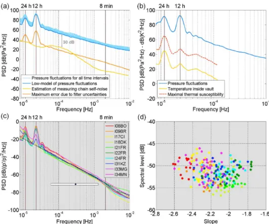
and Sleeman et al. [2006], we evaluated the self‐noise of the measuring chains. For several weeks, three measuring chains were acoustically connected to create a unique air-tight cavity. They were installed in a thermally regulated laboratory to minimize temperature effects. An estimation of their self‐noise low frequency spectrum is displayed in Figure 1a.

1_{CEA, DAM, DIF, Arpajon, France.} 2_{CGGVeritas, Massy, France.}

3_{LATMOS, IPSL, INSU, CNRS, Université Versailles St Quentin,}

UPMC‐Paris 6, Guyancourt, France.

GEOPHYSICAL RESEARCH LETTERS, VOL. 37, L19802,doi:10.1029/2010GL044181, 2010

(3)

[7] To compare this self‐noise with atmospheric pressure

fluctuations at ground level, we computed the power spec-tral density (PSD) of the pressure fluctuations recorded at the I21FR station on twelve‐day time intervals during the entire year 2006. The computations were performed on pres-sure signals digitally corrected from filter effects as will be discussed in section 2.2. In Figure 1a, we can see that the signal‐to‐noise ratio (SNR) between the lowest atmospheric pressure fluctuations and the measuring chain self‐noise exceeds 30 dB in the entire GW range. This demonstrates that pressure fluctuations recorded in the GW frequency range are not significantly affected by the measuring chain self‐noise.

2.2. Transfer Function

[8] Atmospheric pressure fluctuations produced by

infra-sonic wave propagation are several orders of magnitude smaller than those produced by GWs or meteorological processes. To improve data acquisition and processing, the IMS infrasound sensors are designed to work as high gain bandpass filters. This filtering can be acoustic or electronic [Ponceau and Bosca, 2010]. The Martec microbarometers use very stable and accurate analog electronic bandpass fil-ters adjusted in laboratory. As their low cut‐off frequency

is set at 9.8 10−3Hz (specification 0.01 Hz), the entire GW frequency range is attenuated by the filter.

[9] We evaluated the uncertainties of this low cut‐off

frequency using data from field experiments. It was found that the maximum error produced by the variations of this low cut‐off frequency was at least 34 dB lower than the pressure PSD (Figure 1a). This demonstrates that the IMS pressure measurements can be accurately corrected a pos-teriori from filtering effects.

2.3. Thermal Susceptibility

[10] Another source of error at low frequencies is the

thermal susceptibility of the measuring chains. Martec micro-barometers are composed of an aneroid capsule, which is deflected under pressure changes. The capsule deflection is measured with a low noise displacement transducer [Ponceau and Bosca, 2010]. Temperature changes can affect both the transducer and the distance between the transducer and the aneroid capsule. The components of the displacement trans-ducer are chosen for their low susceptibility to temperature. The bond between the aneroid capsule and the displace-ment transducer is manufactured from two materials whose lengths are adjusted in order to minimize temperature effects. This results in microbarometers with a thermal susceptibility lower than 10 Pa.K−1[DASE, 1998].

Figure 1. (a) PSDs of the pressure fluctuations recorded at the central site of the I21FR station for all twelve‐day time intervals in 2006 (light blue, minimum in dark blue), PSD of the measuring chain self‐noise (yellow) and PSD of the max-imum error resulting from the filter uncertainties (orange). (b) PSD of pressure fluctuations recorded by the central micro-barometer of the I21FR station on a twelve‐day time interval (blue), PSD of the temperature inside the vault (yellow) and PSD of the fluctuations that would be produced by a sensor with maximum thermal susceptibility (red). (c) Averaged PSDs computed for ten IMS stations in 2006 and estimation of the average spectral level (black dotted). The white bar shows the fitting domain. The station geographical distribution is plotted in Figure 2c. (d) Slopes and spectral levels (at 3.10−4Hz) estimated on twelve‐day time intervals in 2006.

MARTY ET AL.: USING IMS NETWORK TO STUDY GRAVITY WAVES L19802

L19802

(4)

[11] To estimate the influence of sensor thermal

suscep-tibility on pressure signals, we computed the PSD of the pres-sure fluctuations recorded at the central site of the I21FR station on an arbitrary twelve‐day time interval. We then calculated the PSD of the temperature fluctuations recorded inside the vault by the acquisition unit (Figure 1b). Since the maximum thermal susceptibility of microbarometers is 10 Pa.K−1, the PSD of the error produced by a sensor with the maximum thermal susceptibility is 20 dB above the PSD of temperature fluctuations. As can be seen in Figure 1b, this PSD is at least 25 dB below the average atmospheric pressure fluctuations. This demonstrates that the sensor thermal susceptibility do not significantly affect the pressure signal. Note that we cannot determine the PSD of temperature fluctuations with periods shorter than two hours because the temperature recorded by the acquisition unit is stored with a one‐hour sampling period. However, since vaults are well thermally insulated, temperature fluc-tuations inside sensor measurement cavity will be filtered out all the more as the frequency increases. It follows that the influence of sensor thermal susceptibility on pressure signals will become increasingly negligible for periods shorter than two hours.

3. Gravity Wave Spectra

[12] A large number of theoretical and experimental

studies have analyzed GW spectra in the middle and the upper atmosphere [Fritts and Alexander, 2003]. However, spectra based on ground pressure data and encompassing the entire GW frequency range are rare [e.g., Herron et al., 1969]. We therefore computed the PSD of the relative pres-sure fluctuations (on twelve‐day time intervals) recorded in 2006 by ten IMS stations: I08BO (Bolivia), I09BR (Brazil), I17CI (Côte d’Ivoire), I18DK (Greenland), I21FR (Marque-sas Islands), I22FR (New Caledonia), I24FR (Tahiti), I31KZ (Kazakhstan), I33MG (Madagascar) and I34MN (Mongolia). The stations were selected according to their geographical location and data availability. The averaged PSDs at each fre-quency are plotted in Figure 1c.

[13] Note that it is generally assumed that the GW

fre-quency band ranges from a few minutes to 24 h. This results from the linear theory, which stipulates that the GW intrinsic frequency is bounded between the buoyancy and the Cor-iolis frequencies [Fritts and Alexander, 2003]. However, the buoyancy frequency depends on atmospheric temperature profiles and the Coriolis frequency vanishes at the equator. Moreover, microbarograph networks are fixed in the ter-restrial reference frame and records the apparent frequency of the waves. Gravity wave spectra can therefore be dis-torted through Doppler effects [Fritts and VanZandt, 1987] and the vertical lines plotted at 8 min and 24 h are indica-tions but not precise limits of the GW frequency range.

[14] Despites the possible Doppler distortions and the fact

that stations are installed at different geographical locations and altitudes, we can observe that all PSD nearly collapse on the same line (black dotted) whose slope is about−2.2 in the GW frequency range. It is the first time, to our knowledge, that this expected result, globally related to saturation pro-cesses [Fritts and Alexander, 2003], is observed on such a worldwide scale at the ground. It indeed seems that an averaged universal GW spectrum could be established for the ground surface. Such an empirical model could be used

to improve GW parameterization in global meteorological models. The only clear differences that can be observed between the averaged PSDs are at subharmonic periods of a solar day and at periods shorter than the buoyancy period. The first ones are produced by atmospheric tides and will be discussed in section 4 whereas the other ones are related to atmospheric turbulence in the infrasound frequency range.

[15] To evaluate the variability of slopes and spectral

levels, we fitted all the PSDs calculated on twelve‐day time intervals to straight lines on logarithmic scales. The results presented in Figure 1d show slopes ranging from −2.61 to−1.76 and spectral levels at 3.10−4 Hz from −57 dB to −46 dB. We can observe that the slope range slightly vary with the station position. These results are in agreement with Herron et al. [1969] who estimated monthly‐averaged spectra with slopes ranging from−1 to −2.5 and a spectral level variability lower than 10 dB with a local network of microbarographs.

4. Atmospheric Tides

[16] In section 2.3, we have seen that the influence of

sensor thermal susceptibility was the highest at diurnal and semidiurnal periods. At these two periods, the SNR is approximately the ratio between the amplitude of pressure fluctuations produced by atmospheric tides and the ampli-tude of the spurious fluctuations produced by diurnal tem-perature fluctuation harmonics. It therefore depends on the station geographical location and the period of the year and needs to be evaluated for each IMS station. Atmospheric tides are internal GWs produced by the periodic solar heating of the atmosphere combined with the upward eddy convection of heat from the ground. Their frequencies are harmonics of a solar day with primarily diurnal and semi-diurnal periods. Their impact on atmospheric circulation is important as they cause regular oscillations in atmospheric wind, temperature, and pressure fields up to the mesosphere. The surface pressure oscillations produced by atmospheric tides are often noted Sns with n being the solar day period harmonic and s being the tide wavenumber [e.g., Haurwitz and Cowley, 1973]. Since IMS stations are fixed in the terrestrial reference frame, they cannot detect the non‐ propagating components Sn0.

[17] We analyzed the data recorded in 2006 and 2007 by

the ten IMS stations described in section 3. To characterize the monthly‐averaged diurnal and semidiurnal pressure oscil-lations produced at these ten stations, we began by applying the superimposed epoch method [Panofsky and Brier, 1958] on a diurnal time interval. From the resulting signal, we selected the diurnal and semidiurnal spectral complex com-ponents. These two components respectively corresponds to S1and S2’s complex amplitudes.

[18] The Figure 2a presents the amplitude of S1and S2(on a logarithmic scale) recorded by the four microbarographs of the I21FR station during 2006 and 2007. The standard deviation between the tide amplitudes recorded by the four measuring chains is also displayed. The corresponding rel-ative standard deviation (RSD) is less than 2.2% for S1and 0.7% for S2, which confirms the good SNR evaluated in section 2 for the I21FR station. The RSD was calculated monthly for the ten listed IMS stations in 2006 and 2007. It never exceed 10% except for the I18DK (Greenland), for which S1’s RSD reached 33% (Figure 2b). This can be

(5)

related to the weakness of the atmospheric tide amplitude in polar regions. It shows that sensor thermal susceptibility can potentially affect the pressure signal at diurnal period.

[19] In Figures 2a and 2b, we can see that the variability

of S2’s amplitude is globally the same in 2006 and 2007, whereas no tendency appears for S1’s amplitude. This might be due to the fact that S2is essentially produced by the radi-ative heating of the stratospheric ozone while S1is mainly produced by the radiative heating of tropospheric water vapor and the ground [Chapman and Lindzen, 1970]. S2’s amplitude is therefore much more homogeneously distrib-uted and stable from year to year than S1’s. Figures 2c and 2d respectively presents the complex amplitudes of S1and S2 recorded at ten IMS stations in 2006 and 2007. To easily compare the pressure oscillations recorded at the different stations, the phases of the complex amplitudes were con-verted from coordinated universal time (UTC) to local solar time (LST). They represent the time of the pressure maximum.

[20] In Figure 2d we can see that the amplitude and the

phase of S2 are very stable throughout the year and from year to year. S2mainly peaks between 0900 and 1030 LST (and between 2100 and 2230 LST) except for the North Greenland station, where peaks occur between 0500 and 0800 (and between 1700 and 2000 LST). S2’s amplitude decreases poleward with an average amplitude of 90–130 Pa for tropical stations. These results are in full agreement with previous global scale observations [e.g., Dai and Wang, 1999, Figures 8 and 10]. The Côte d’Ivoire station is the only station for which S2’s amplitude is significantly larger than the

average amplitudes obtained by Dai and Wang [1999]. This difference may be explained by the fact that we only pro-cessed two years of data whereas Dai and Wang [1999] presented values averaged over 20 years.

[21] In Figure 2c, we can see that S1’s distribution is much broader than S2’s with a significant amplitude and phase var-iability for continental stations. S1’s phase instability might be due to meteorological processes that produce pressure fluctuations with similar amplitudes when S1’s amplitude is weak. S1generally peaks between 0300 and 0800 LST. This is in agreement with Trenberth [1977] and Kong [1995] which found peak times respectively around 0500–0600 over New Zealand and 0400–0840 LST over Australia. Dai and Wang [1999] obtained peak times around 0600–0800 for tropical regions, which is a little bit later than our aver-age peak time. They however mentioned that S1’s phase considerably varied on small scales and from year to year; a phenomenon also pointed out by Trenberth [1977] and Kong [1995].

5. Conclusion and Prospects

[22] In this letter, we demonstrated that the pressure

fluctuations recorded by most IMS infrasound stations could be used to study GWs. We showed that one of the main sources of error at low frequencies was related to sensor thermal susceptibility and that its influence at the diurnal period needed to be evaluated for each IMS station. Since IMS stations are regularly calibrated and record pressure fluctuations all over the Earth’s surface, they provide an accurate and reliable stream of data useable to study the Figure 2. (a, b) Absolute amplitude of S1(purple‐blue circles) and S2(yellow‐red circles) recorded by the four sensors of the I21FR and I18DK stations in 2006 and 2007. The mean and the standard deviation are respectively represented by the solid and dashed curves. (c, d) Complex amplitudes of S1and S2recorded at ten IMS stations in 2006 (circles) and 2007 (triangles).

L19802

(6)

entire GW band on a worldwide scale. We thus investigated the atmospheric background fluctuations produced at ten IMS stations and showed a striking similarity between all the GW spectra despite the station broad geographical dis-tribution. We therefore suggested that IMS data could be used to compute empirical models for atmospheric pressure fluctuations and improve GW parameterization in meteo-rological models.

[23] We also studied the diurnal and semidiurnal surface

pressure oscillations produced by atmospheric tides and found results in good agreement with previous models and observations. Due to their accuracy and high temporal res-olution, IMS data could be integrated in current empirical models and allow to study higher tide harmonics (unlike previous studies which were often limited to the two first harmonics [e.g., Haurwitz and Cowley, 1973; Dai and Wang, 1999]). Although within this letter we presented an exam-ple of planetary wave detection, we would like to point out that the IMS pressure measurements can also be used to study mesoscale GWs. The geometry of the measuring chains within each IMS station is indeed well‐adapted for the characterization of such waves and is similar to that used by previous measurement campaigns [e.g., Hauf et al., 1996; Rees et al., 2000]. Since the first IMS infrasound stations were installed almost ten years ago with now more than forty stations being operational, the analysis of IMS data in the GW range could therefore improve our knowl-edge of GW sources, propagation, reflection and saturation processes. Finally, we would like to mention that the detection of pressure fluctuations produced by semidiurnal tides can be an excellent means to monitor the performance of IMS stations, since semidiurnal pressure oscillations are accurately detected all over the Earth’s surface on a daily basis.

[24] Acknowledgments. The authors would like to thank C. Haynes for his useful comments.

References

Balachandran, N. K. (1980), Gravity waves from thunderstorms, Mon. Weather Rev., 108, 804.

Blanc, E., A. L. Pichon, L. Ceranna, T. Farges, J. Marty, and P. Herry (2010), Global Scale Monitoring of Acoustic and Gravity Waves for the Study of the Atmospheric Dynamics, in Infrasound Monitoring for Atmospheric Studies, pp. 647–664, Springer, New York.

Chapman, S., and R. S. Lindzen (1970), Atmospheric Tides, 200 pp., D. Reidel, Dordrecht, Netherlands.

Dai, A., and J. Wang (1999), Diurnal and semidiurnal tides in global sur-face pressure fields, J. Atmos. Sci., 56, 3874–3891.

DASE (1998), Microbarometer MB2000 Technical Manual, CEA, Arpajon, France.

DASE (2008), Authenticated Alpilles Technical Manual, CEA, Arpajon, France.

Evers, L., L. Ceranna, H. Haak, A. L. Pichon, and R. Whitaker (2007), A seismoacoustic analysis of the gas‐pipeline explosion near Ghislenghien in Belgium, Bull. Seismol. Soc. Am., 97, 417–425.

Farges, T., A. Le Pichon, E. Blanc, S. Perez, and B. Alcoverro (2003), Response of the lower atmosphere and the ionosphere to the eclipse of August 11, 1999, J. Atmos. Sol. Terr. Phys., 65, 717–726.

Fritts, D. C., and M. J. Alexander (2003), Gravity wave dynamics and effects in the middle atmosphere, Rev. Geophys., 41(1), 1003, doi:10.1029/ 2001RG000106.

Fritts, D. C., and T. E. VanZandt (1987), Effects of Doppler shifting on the frequency spectra of atmospheric gravity waves, J. Geophys. Res., 92(D8), 9723–9732.

Hauf, T., U. Finke, J. Neisser, G. Gull, and J. G. Stangenberg (1996), A ground‐based network for atmospheric pressure fluctuations, J. Atmos. Oceanic Technol., 13, 1001–1023.

Haurwitz, B., and D. Cowley (1973), The diurnal and semidiurnal baromet-ric oscillations, global distribution and annual variation, Pure Appl. Geo-phys., 102, 193–222.

Herron, T. J., I. Tolstoy, and D. W. Kraft (1969), Atmospheric Pressure Background Fluctuations in the Mesoscale Range, J. Geophys. Res., 74, 1321–1329.

Holcomb, L. G. (1989), A direct method for calculating instrument noise levels in side‐by‐side seismometer evaluations, U.S. Geol. Surv. Open File Rep., 89–214.

Kong, C.‐W. (1995), Diurnal pressure variations over continental Australia, Aust. Meteorol. Mag., 44, 165–175.

Le Pichon, A., J. M. Guérin, E. Blanc, and D. Reymond (2002), Trail in the atmosphere of the 29 December 2000 meteor as recorded in Tahiti: Char-acteristics and trajectory reconstitution, J. Geophys. Res., 107(D23), 4709, doi:10.1029/2001JD001283.

Le Pichon, A., E. Blanc, and D. Drob (2005), Probing high‐altitude winds using infrasound, J. Geophys. Res., 110, D20104, doi:10.1029/ 2005JD006020.

Panofsky, H. A., and G. W. Brier (1958), Some Applications of Statistics to Meteorology, Pa. State Univ., University Park.

Ponceau, D., and L. Bosca (2010), Specifications of low‐noise broadband microbarometers, in Infrasound Monitoring for Atmospheric Studies, pp. 119–140, Springer, New York.

Rees, J. M., J. C. W. Denholm‐Price, J. C. King, and P. S. Anderson (2000), A climatological study of internal gravity waves in the atmo-spheric boundary layer overlying the brunt ice shelf, Antarctica, J. Atmos. Sci., 57, 511–526.

Sleeman, R., A. van Wettum, and J. Trampert (2006), Three‐channel correlation analysis: A new technique to measure instrumental noise of digitizers and seismic sensors, Bull. Seismol. Soc. Am., 96, 258–271. Trenberth, K. E. (1977), Surface atmospheric tides in New Zealand, N. Z. J.

Sci., 20, 339–356.

F. Dalaudier, LATMOS, IPSL, INSU, CNRS, Université Versailles St Quentin, UPMC‐Paris 6, F‐78280 Guyancourt CEDEX, France.

J. Marty, CEA, DAM, DIF, F‐91297 Arpajon CEDEX, France. (julien. [email protected])

D. Ponceau, CGGVeritas, 1, rue Léon Migaux, F‐91341 Massy CEDEX, France.