Disentangling the effects of external perturbations on coexistence and priority effects

(1)

Supporting Information for

Disentangling the effects of external perturbations on

coexistence and priority effects

Chuliang Song1_{, Rudolf P. Rohr}2_{, David Vasseur}4_{, Serguei Saavedra}1

1_{Department of Civil and Environmental Engineering, MIT,}

77 Massachusetts Av., 02139 Cambridge, MA, USA

2_{Department of Biology – Ecology and Evolution, University of Fribourg,}

Chemin du Musée 10, CH-1700 Fribourg, Switzerland

3_{Department of Ecology and Evolutionary Biology, Yale University,}

(2)

A Equivalent parameterizations

It is worth noting that several mathematically equivalent parameterizations have been used to describe the LV dynamics of 2-competing species (Case, 2000). Yet, regardless of model parameterization, the conditions leading to coexistence or priority effects are equivalent under the Structural Approach. For example, in addition to the r formalism (Eq. 1) and MCT for-malism (Eq. 4), the LV model can also be expressed in terms of carrying capacities (Vander-meer, 1975). In this other parameterization—what is known as the K-formalism, the carrying

capacities Ki are made explicit in the model as

Y _ _ ] _ _ [ dN1 dt = N1 r1 K1(K1≠ N1≠ a12N2) dN₂ dt = N2 r₂ K2(K2≠ a21N1≠ N2). (S1)

Recall that the carrying capacity Ki of species i is computed as Ki = ri/–ii. It corresponds

to the abundance at equilibrium when the species grows in the absence of competition strength.

Note that the carrying capacity is well defined only if ri > 0, i.e., the species can grow in

monoculture (Gabriel et al., 2005). To be equivalent to Eq. (1), the competition strength

must be standardized by the intraspecific competition, i.e., aij = –ij/–ii. Note that aij is

tra-ditionally called the niche overlap of species j on species i (Case, 2000). In the K-formalism, the condition for coexistence (Eq. 2) reads as

ﬂ < K2 K1 Ú_a 12 a21 < 1 ﬂ, (S2)

and the condition for priority effects reads as ﬂ > K2 K1 Ú_a 12 a21 > 1 ﬂ. (S3)

These two sets of inequalities are very similar to those in the r-formalism (Eqs. 2 and 3).

Notice that ri is replaced by Ki and Qj by aij. Replacing the new parametrization into Eqn.

5, the niche overlap is given by ﬂ = Ôa12a21, which reveals that the niche overlap ﬂ defined in

MCT is, in fact, the geometric average of the niche overlap aij of the two competing species.

Thus, the representation of the dynamical behavior of the LV model can be drawn in the

2-dimensional space made by the species fitness (Ÿi = ri/Ô–ii–ij), the carrying capacities

(Ki = ri/aii), or the intrinsic growth rates (ri) (Case 1999; Fig. S1). These representations

in the space of intrinsic growth rates are the core concept behind the structural approach (Saavedra et al., 2017b). That is, Figure S1 shows that all these representations are

conceptu-ally equivalent to describe the range (as an algebraic cone) of intrinsic growth rates leading to a given qualitative behavior (either coexistence or priority effects).

(3)

A B C D E F

Coe

xist

enc

e

Pr

ior

ity e

ffec

ts

Species 1 fitness(κ1=r1/ α11α12) Specie s2 fitness (κ2 = r2 / α22 α21 ) Fitness space

Species 1 carrying capacity(K1=r1/α11)

Specie s2 carryin g capacity (K2 = r2 /α22 )

Carrying capacity space

Species 1 intrinsic growth rate(r1)

Specie s2 intrinsi c growt h rate (r2 )

Intinsic growth rate space

Species 1 fitness(κ1=r1/ α11α12) Specie s2 fitness (κ2 = r2 / α22 α21 )

Species 1 carrying capacity(K1=r1/α11)

Specie s2 carryin g capacity (K2 = r2 /α22 )

Species 1 intrinsic growth rate(r1)

Specie s2 intrinsi c growt h rate (r2 )

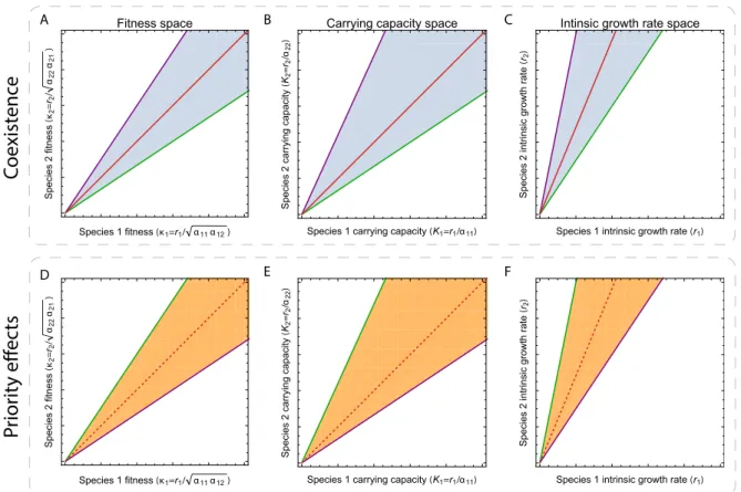
Figure S1: Space of intrinsic growth rates for coexistence and priority effects. The dynam-ics correspond to the Lotka-Volterra model (Eq. 1). These panels represent the range of intrinsic growth rates—species fitness (panels A and D), carrying capacities (panels B and E), and intrinsic growth rates (panels C and F)—leading to coexistence or priority effects. Whether we can be in the presence of coexistence or priority effects is determined by the

stability-instability inequality, i.e., –22/–12 > –21/–11 for coexistence (panels A and C) or

–22/–12 < –21/–11 for priority effects (panels D and F). The slopes (–21/–11 in green and

–22/–12in purple) of the two lines determining the coexistence (or priority effects) cone are

computed from the competition strengths. Actually, these four panels are a simple geometric representation of the inequalities expressed in Eqs. (2) and (3). The red line represents the fitness equivalence line, and in dashed, its extension to priority effects.

(4)

B Importance of intrinsic growth rates

In the MCT formalism (Eq. 4), intrinsic growth rates do not play any explicit role in either feasibility nor stability. However, this is a special property of 2-species ODEs guaranteed by the Poincaré–Bendixson theorem (Strogatz, 2014). Yet, a well-known counter-example to the fact that intrinsic growth rates do impact the dynamics in other dimensions is the discrete logistic growth dynamics of a single species,

Nt+1= rNt(1 ≠ Nt), (S4)

where increasing the intrinsic growth rate r would move the system from staying at a fixed equilibrium to a chaotic dynamics. Moreover, it is rather easy to show counter-examples in systems with more than 2 species. For example, consider the following 4-species competi-tion ODEs with fixed interaccompeti-tion matrix (written following MCT formalism). The governing population dynamics are (Vano et al., 2006)

dN dt = diag(r)diag(N)(1 ≠ Q c c c a 1 1.09 1.52 0 0 1 0.44 1.36 2.33 0 1 0.47 1.21 0.51 0.35 1 R d d d bN). (S5)

where N = (N1, N2, N3, N4) is the vector of species abundances.

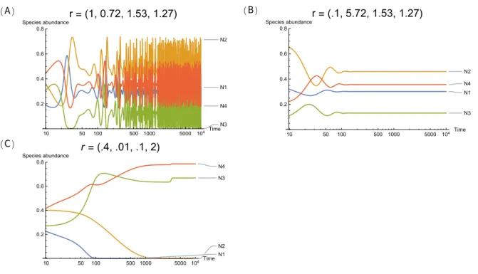
Figure S2A shows that the system exhibits chaotic behavior with intrinsic growth rates r = (1, 0.72, 1.52, 1.27), Figure S2B shows that the system exhibits a point attractor with intrinsic

growth rates r = (0.1, 5.72, 1.53, 1.27), and Figure S2C shows that the system exhibits species extinction with intrinsic growth rates r = (0.4, 0.01, 0.1, 2). This illustrates the importance of intrinsic growth rates in population dynamics even under the MCT formalism.

(A) N1 N2 N3 N4 10 50 100 500 1000 5000 104Time 0.2 0.4 0.6 0.8 Species abundancer = (1, 0.72, 1.53, 1.27) (B) N1 N2 N3 N4 10 50 100 500 1000 5000 104 Time 0.2 0.4 0.6 0.8 Species abundancer = (.1, 5.72, 1.53, 1.27) (C) N2 N3 N4 N1 10 50 100 500 1000 5000 104Time 0.2 0.4 0.6 0.8 Species abundance r = (.4, .01, .1, 2)

Figure S2: Intrinsic growth rates impact population dynamics. All the simulations are gov-erned by the same initial conditions and the same interaction matrix, but the intrinsic grow rates. Panel A exhibits chaotic behavior, Panel B exhibits a point attractor, and Panel C exhibits species extinction. The x axis is on the log ratio.

(5)

C Structural Approach and priority effects

The Structural Approach (SA) has been defined as the structural stability of coexistence under changes in intrinsic growth rates (Saavedra et al., 2017b). Here, we show how SA can be naturally extended to priority effects.

Theorem S1. The structural stability of priority effects under changes in intrinsic growth

rates can be computed as = arccos_Ô Q1+Q2

1+Q2 1Ô1+Q22

Proof. Criteria for stable coexistence is Q₁< r2

r1 <

1

Q2 (S6)

and the criteria for priority effects is 1 Q2 <

r2

r1 < Q1 (S7)

Thus, the transition from stable coexistence to priority effects can be seen as 1

Q2 ‘æ Q1 (S8)

Q1 ‘æ 1

Q2 (S9)

With the triangulate equality that

tan – ≠ tan —

1 + tan – tan — = 1 + 1/(tan – tan —)1/ tan — ≠ 1/ tan – (S10)

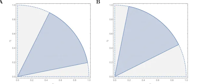
This shows that the normalized solid angle remains the same after the transition. With

elementary trigonometric transformation, we have the result shown in Fig. S3.

A 0.0 0.2 0.4 0.6 0.8 1.0 0.0 0.2 0.4 0.6 0.8 1.0 r1 r2 B 0.0 0.2 0.4 0.6 0.8 1.0 0.0 0.2 0.4 0.6 0.8 1.0 r1 r2

Figure S3: Cartoon of the proof. The figure shows how the transformation alters the rela-tive position of the structural stability region but keeps the size fixed. Panel A represents coexistence, while Panel B represents priority effects.

(6)

D Formal combination of MCT and SA

To simplify the derivation of the combination of MCT and SA, let us denote the fitness ratio

r2

r1

Ò

Q2

Q1 as „ and the ratio of intrinsic growth rates

r2

r1 as µ.

D.1 Stabilizing mechanism and SA

Let us fix the fitness ratio „ as a positive constant. Then Q2 = „2µ≠2Q1, and the niche

overlap can be written as

ﬂ=Q1Q2= „µ≠1Q1, (S11)

which implies that

cos =  ﬂ(„≠2µ2+ 1)

1 + „≠2_µ2_ﬂ2_ﬂ2+ „≠2_u2. (S12)

Looking at the conditions in ﬂ that increase (the region of coexistence or priority effects)

we have ˆcos ˆfl = „≠2µ2!1 ≠ fl4"!„≠2µ2+ 1" („≠2_µ2+ fl2)3/2(„≠2_µ2_fl2+ 1)3/2, which is I >0, if fl < 1 <0, if fl > 1, . (S13)

which implies that decreases as niche overlap ﬂ increases under coexistence (ﬂ < 1), and

increases as niche overlap ﬂ increases under priority effects (ﬂ > 1.). Similarly, looking at the

conditions in µ that increase we have

ˆcos ˆµ = „≠2µfl!fl2≠ 1"2!„≠2µ2≠ 1" („≠2_µ2+ fl2)3/2(„≠2_µ2_fl2+ 1)3/2, which is I >0, if Q1 > Q2 <0, if Q1 < Q2, . (S14)

Thus, when „≠2_µ2 _> _{1 (i.e., Q}₁ _{> Q}₂_), _{would increase if µ =} r2

r1 decreases; and when

„≠2µ2 < 1 (i.e., Q1 < Q2), would increase if µ = r_r2₁ increases. This pattern is the same

regardless of whether looking at coexistence or priority effects. D.2 Equalizing mechanism and SA

Let us fix the niche overlap ﬂ as a positive constant. Without loss of generality, we assume

that fitness ratio „ Ø 1. Then Q1 = ﬂµ„≠1, Q2 = ﬂµ≠1„. Unlike the stabilizing mechanism,

the equalizing mechanism is not always well-defined as feasibility is not always satisfied —

µhas to lie within the feasibility domain spanned by (Q₁,1) and (1, Q₂). Hence, we define

:= 0 when feasibility is violated. Focusing on priority effects we have

cos =  ﬂ(µ2+ „2)

„2+ fl2µ2µ2+ fl2„2,where fl

≠1_µ2_{< „ < ﬂµ}2 _(S15)

Note that the condition ﬂ≠1_µ2 _{< „ < ﬂµ}2 _{is equivalent to the feasibility condition} 1

Q1 < µ <

Q2. Similarly, for coexistence we have

cos =  ﬂ(µ2+ „2)

„2+ fl2µ2µ2+ fl2„2,where flµ

2_{< „ < ﬂ}≠1_µ2 _(S16)

Focusing only on non-trivial (i.e., cos ”= 1), the derivative of cos is

ˆcos

(7)

which impels that decreases when „ > µ and increases otherwise in both coexistence and priority effects.

Furthermore, when are fixed, then

„2=

µ2csc2( )

3

2!fl4+ 1"cos2( ) ≠ 4fl2+Ô2!fl2_{≠ 1}"cos( )Òfl4+ (fl2+ 1)2cos(2 ) ≠ 6fl2+ 1

4

4ﬂ2 .

(S18)

The conditions above imply that Q1 and Q2 do not depend on µ. Note that in the extreme

case when reaches its maximum (i.e., „ = µ, or, equivalently, Q1 = Q2), the maximum of

is arccos1_ﬂ22ﬂ₊₁

2

(8)

E Ratios of intrinsic growth rates and maximum solid angle

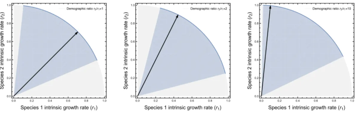
Figure 4 shows that different ratios of intrinsic growth rates r2/r1 can yield the same

maxi-mum solid angle . While different ratios of intrinsic growth rates r2/r1 would have the same

aggregated tolerance to random perturbations (i.e. ), they have different tolerances to

direc-tional perturbations. Figure S4 shows the three ratios r2/r1 = 1, 2, 10 with their associated

maximum . When r2/r1 = 1, the tolerances to directional perturbations (i.e. distances

to the boundaries) are similar. However, when r2/r1 increases, the tolerances to directional

perturbations shows a stronger trade-off.

Demographic ratio r2/r1=1 0.0 0.2 0.4 0.6 0.8 1.0 0.0 0.2 0.4 0.6 0.8 1.0

Species 1 intrinsic growth rate (r1)

S pecies 2 int rinsic growt h rat e (r2 ) Demographic ratio r2/r1=2 0.0 0.2 0.4 0.6 0.8 1.0 0.0 0.2 0.4 0.6 0.8 1.0

S pecies 2 int rinsic growt h rat e (r2 ) Demographic ratio r2/r1=10 0.0 0.2 0.4 0.6 0.8 1.0 0.0 0.2 0.4 0.6 0.8 1.0

S pecies 2 int rinsic growt h rat e (r2 )

Figure S4: Different tolerances to directional perturbations with the same . The two axes denote the intrinsic growth rates of two species. The blue region denotes the feasibility do-main. The black line denotes the ratio of intrinsic growth rates (values in upper-right). As the ratio of intrinsic growth rates deviates more from 1, the system is more robust to pertur-bation upon one boundary and less robust to perturpertur-bation upon the other boundary.

(9)

F Annual plant model

This section discusses how to apply MCT and SA on an the annual plant model (Godoy & Levine, 2014). A more detailed disucssion can be found in Godoy & Levine (2014); Godoy et al. (2014); Saavedra et al. (2017b). The annual plant model reads as

dNi,t+1 dt = (1 ≠ gi)siNi,t+ gi⁄iNi,t 1 +qn j=1˜–ijgjNj,t , (S19)

where gi is the germination rate, si is the seed survival probability, ⁄i is the fecundity rate,

and ˜–ij is the competition strength (relative reduction in per capita growth rate). After

alge-braic manipulation, the equilibrium Nú

i can be expressed as a linear equation:

gi⁄ 1 ≠ (1 ≠ gi)si ≠ 1 = n ÿ j=1 ˜–ijgjNjú. (S20)

Then, Eq. 1 can be achieved via re-parametrization

ri :=

gi⁄

1 ≠ (1 ≠ gi)si ≠ 1 (S21)

(10)

G Hypothesis testing for field data

Here we performed a hypothesis testing to show that there is a significant statistical tendency

to increase the feasibility domain rather than increasing the fitness equivalence in the field

data (Figure 5B-C). Recall that the maximization of the former implies higher pressures in intrinsic growth rates, while the maximization of the latter implies higher pressures in competition strengths. Specifically, we established two hypotheses:

H0: the tolerance to perturbation in competition strength is maximized (S23)

H1: the tolerance to perturbation in intrinsic growth rates is maximized (S24)

(S25) To formalize this problem, it is equivalent to ask whether points in Figure 5B-C are closer

to the fitness equivalence line or to the maximizing line. Let us denote the distance to

the fitness equivalence line as d1 and the distance to the maximizing line as d2. Then, the

hypotheses are equivalent to

H0 : d2/d1 <1 (S26)

H1 : d2/d1 >1 (S27)

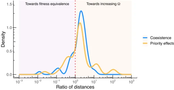
Figure S5 shows the distribution of the log ratios of distances d2/d1 in the empirical data

set. Then, we ran Wilcoxon signed-rank test on the two hypotheses. For coexistence, we

found that H0 has a p value of 1 and H1 has a p value of 3.049 ◊ 10≠7. Similalry, for priority

effects, we found that H0 has a p value of 1, and H0 has a p of value 0.0001009. Therefore, we

rejected the null hypothesis, and concluded there is a tendency to maximize the tolerance to perturbations in intrinsic growth rates.

Towards fitness equivalence Towards increasing Ω

0.0 0.5 1.0 1.5 10−3 10−2 10−1 100 101 102 103 Ratio of distances Density Coexistence Priority effects

Figure S5: This figure shows the distribution of the ratio of distances d2/d1 for coexistence

(in blue) and priority effects (in orange) in the annual plants assemblages. The dotted red line