Correct-by-construction finite field arithmetic in Coq

Correct-by-Construction Finite Field Arithmetic in

Coq

by

Jade Philipoom

Submitted to the Department of Electrical Engineering and Computer

Science

in partial fulfillment of the requirements for the degree of

Master of Engineering in Computer Science

at the

MASSACHUSETTS INSTITUTE OF TECHNOLOGY

February 2018

c

○ Massachusetts Institute of Technology 2018. All rights reserved.

Author . . . .

Department of Electrical Engineering and Computer Science

February 2, 2018

Certified by . . . .

Adam Chlipala

Associate Professor of Electrical Engineering and Computer Science

Thesis Supervisor

Accepted by . . . .

Chris Terman

Chairman, Master of Engineering Thesis Committee

Correct-by-Construction Finite Field Arithmetic in Coq

by

Jade Philipoom

Submitted to the Department of Electrical Engineering and Computer Science on February 2, 2018, in partial fulfillment of the

requirements for the degree of

Master of Engineering in Computer Science

Abstract

Elliptic-curve cryptography code, although based on elegant and concise mathemat-ical procedures, often becomes long and complex due to speed optimizations. This statement is especially true for the specialized finite-field libraries used for ECC code, resulting in frequent implementation bugs. I describe the methodologies used to cre-ate a Coq framework that genercre-ates implementations of finite-field arithmetic routines along with proofs of their correctness, given nothing but the modulus.

Thesis Supervisor: Adam Chlipala

Contents

1 Related Work 13

1.1 ECC Code Verification . . . 14

1.1.1 Cryptol and SAW . . . 14

1.1.2 HACL* . . . 15

1.1.3 verify25519 . . . 15

1.2 Bignum Arithmetic Verification . . . 16

1.2.1 gfverif . . . 16

1.3 Verified Bignums . . . 16

1.4 Adjacent Work . . . 17

1.4.1 Protocol Verification . . . 17

1.4.2 Compilers and Translation Validators . . . 17

2 Mathematical Background 19 2.1 Modular Reduction . . . 19

2.1.1 Generalized Mersenne Reduction . . . 20

2.1.2 Montgomery Reduction . . . 22

2.2 Integer Representation . . . 23

2.2.1 Unsaturated Digits . . . 23

2.2.2 Mixed-Radix Bases . . . 25

3 Representing Multidigit Integers in Coq 27 3.1 Unsaturated . . . 27

3.1.2 Associational and Positional Representations . . . 32 3.2 Saturated . . . 37 4 Summary of Operations 41 4.1 Unsaturated . . . 41 4.2 Saturated . . . 44 4.3 Other . . . 46

5 Producing Parameter-Specific Code 49 5.1 Selecting Parameters . . . 50

5.2 Partial Evaluation . . . 52

5.2.1 Synthesis Mode . . . 52

5.2.2 Marking Runtime Operations . . . 53

5.2.3 Continuation-Passing Style . . . 54

5.3 Linearization and Constant-Folding . . . 57

5.4 Bounds Inference . . . 58

6 Extending with New Arithmetic Techniques 59 6.1 Algorithm . . . 59

6.2 Implementation . . . 60

6.3 Overall Effort of Extension . . . 62

Introduction

Cryptography is only becoming more necessary in the modern world, as it becomes clear that communicating with other individuals over the internet exposes users to

governments, companies, and other malicious actors who are eager to make use of

such broadcasts. Most internet traffic is now encrypted, and the world would be a better place if that cryptography were stronger and more ubiquitous. However, these

goals can be at odds. Ubiquitous encryption means that cryptographic routines are run very often, for instance on every connection with a website. This means that

whoever is running the web server has a strong incentive to push for faster code. Faster code, though, often includes very nontrivial optimizations that make the code

less easy to audit, and prone to tricky implementation bugs. This work is part of a project that uses a mathematical proof assistant, Coq, to produce elliptic-curve

cryptography (ECC) code that is both fast and certifiably free of implementation error. Although the larger project has a scope ranging from elliptic-curve

mathemat-ical properties all the way to assembly-like C code, the work described in this thesis focuses specifically on crafting simplified functional versions of performance-sensitive

finite-field arithmetic routines.

To motivate design decisions on this project, we (primarily my colleague Andres Erbsen) conducted an informal survey of project bug trackers and other internet

sources, which is summarized in Figure 0-1. Interesting to note here is that, of the 28 bugs we looked at, 20 are mistakes in correctly handling the complicated

finite-field arithmetic routines (encompassing three categories in the figure: Carrying, Canonicalization, and Misc. Number System). The distribution reflects the fact

Reference Specification Implementation Defect Carrying

go#13515 Modular exponentiation uintptr-sized Montgomery form, Go

carry handling

NaCl ed25519 (p.2) F25519 mul, square 64-bit pseudo-Mersenne, AMD64 carry handling

openssl#ef5c9b11 Modular exponentiation 64-bit Montgomery form, AMD64

carry handling

openssl#74acf42c Poly1305 multiple implementations carry handling

nettle#09e3ce4d secp-256r1 modular reduc-tion

carry handling

CVE-2017-3732 𝑥2_{mod 𝑚 Montgomery form, AMD64}

as-sembly

carry, exploitable

openssl#1593 P384 modular reduction carry handling carry, exploitable

tweetnacl-U32 irrelevant bit-twiddly C ‘sizeof(long)!=32‘

Canonicalization

donna#8edc799f GF(2255_{− 19) internal to}

wire

32-bit pseudo-Mersenne, C non-canonical

openssl#c2633b8f a + b mod p256 Montgomery form, AMD64 as-sembly

non-canonical

tweetnacl-m15 GF(2255− 19) freeze bit-twiddly C bounds? typo?

Misc. number system

openssl#3607 P256 field element squar-ing

64-bit Montgomery form, AMD64

limb overflow

openssl#0c687d7e Poly1305 32-bit pseudo-Mersenne, x86 and ARM

bad truncation

CVE-2014-3570 Bignum squaring asm limb overflow

ic#237002094 Barrett reduction for p256 1 conditional subtraction instead of 2

no counterexample

go#fa09811d poly1305 reduction AMD64 asm, missing subtrac-tion of 3

found quickly

openssl#a970db05 Poly1305 Lazy reduction in x86 asm lost bit 59

openssl#6825d74b Poly1305 AVX2 addition and reduction bounds?

ed25519.py Ed25519 accepts signatures other impls

reject

missing ℎ mod 𝑙

bitcoin#eed71d85 ECDSA-secp256k1 x*B mixed addition Jacobian+Affine missing case Elliptic Curves

openjdk#01781d7e EC scalarmult mixed addition Jacobian+Affine missing case

jose-adobe ECDH-ES 5 libraries not on curve

invalid-curve NIST ECDH Irrelevant not on curve

end-to-end#340 Curve25519 library twisted Edwards coordinates (0, 1) = ∞

openssl#59dfcabf Weier. affine <-> Jaco-bian

Montgomery form, AMD64 and C

∞ confusion Crypto Primitives

socat#7 DH in Z*p irrelevant non-prime 𝑝

CVE-2006-4339 RSA-PKCS-1 sig. verifi-cation

irrelevant padding check

CryptoNote Anti-double-spending tag additive curve25519 curve point missed order(𝑃 ) ̸= 𝑙

been subject to extremely tricky optimizations. Elliptic-curve cryptography code often uses complex representations for finite-field elements, and avoiding over- or

underflow requires tracking very precise upper and lower bounds in one’s head. It is unsurprising, therefore, that humans make arithmetic errors and fail to account for

some of the many edge cases. Historically, computers have proven much more reliable than humans at those tasks. Therefore, having a computer produce and check the

code has the potential to drastically reduce error rates.

To understand various design decisions described in this document, it is helpful

to note the three main goals that have guided the project since its inception:

∙ Scope: our proofs should be as deep as possible. Currently, we can verify from high-level functional specifications in terms of elliptic curves down to straight-line, assembly-like C.

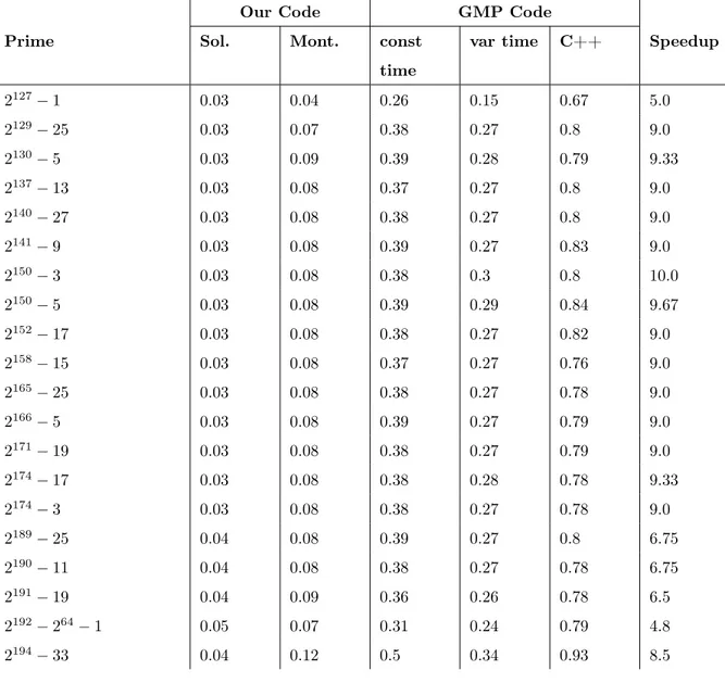
∙ Speed: the code we produce must be fast enough to be competitive with real-world C implementations, which means making use of a variety of nontrivial optimizations. Comparing to specialized C implementations, we come in around

5% slower than donna-c64 and significantly faster than OpenSSL C. We are still roughly 20% slower than hand-optimized assembly, but we achieve between a

1.2 and 10× speedup (depending on the prime) compared to reasonable imple-mentations using libgmp, a fast arbitrary-precision integer library. Figure 0-2

shows our performance compared to the libgmp implementations for various primes. For the full benchmark data, see Appendix A.

∙ Effort: we want to prove as many things as we can once-and-for-all, so that changing parameters (for instance, changing curves) will not require any man-ual work. Currently, it is possible to generate new finite-field operations by

inputting only a prime; the rest is automatic.

This document is organized as follows. Chapter 1 details various pieces of related work to help set an academic context and provide insight into the design space.

128 192 256 320 384 448 512 0 0.5 1 1.5 log2(prime) Time (seconds

) 64-Bit Field Arithmetic Benchmarks

GMP mpn_sec API GMP mpn API this project 128 192 256 320 384 448 512 0 5 10 15 log2(prime) Time (second s)

32-Bit Field Arithmetic Benchmarks

GMP mpn_sec API GMP mpn API this project

Figure 0-2: Performance comparison of our generated C code vs. handwritten using libgmp

Chapter 3 describes our overall strategies for how to encode those ideas in Coq.

Chapter 4 provides a list of all the operations defined by the finite-field arithmetic library and gives some detail on the implementation of each one. Chapter 5 describes

how we transform proven-correct general code into fast low-level implementations. Finally, Chapter 6 remarks on how the library can be extended with new techniques,

using Karatsuba multiplication as an example.

Individual Contributions

The project described in this thesis is a collaboration between myself, Andres Erbsen, and Jason Gross, all advised by Professor Adam Chlipala. For an early version of

the library, Robert Sloan built a low-level compilation pipeline which ended up being replaced as the requirements matured.

This document will describe the finite-field arithmetic section of the library only, which was designed collaboratively by myself and Andres but subsequently developed

primarily by me. The low-level compilation work described in Chapter 5 was primarily done by Jason, also with design input from Andres. Some text about related work

jointly authored paper. Andres’s thesis also influenced my writing about related work in Chapter 1.

Chapter 1

Related Work

Numerous other projects in this general domain are relevant to the academic context

of this work and serve as a basis of comparison for our strategies, goals, and results. These can be grouped into two broad categories:

∙ ECC code verification efforts (Section 1.1), which are domain-specific projects that aim for guarantees of functional correctness.

∙ Bignum arithmetic verification efforts (Section 1.2), which are not specific to ECC but are highly useful for checking its most important properties. This is particularly relevant to verified finite-field arithmetic, the section of our project

that this document describes.

In Section 1.4, we will also discuss some adjacent domains: protocol verification

and verified compilers/translation validators. Such projects do not have much overlap with our work but are plausible connecting points for a truly end-to-end proof, which

could provide guarantees all the way from security properties formalized in the style of academic cryptography down to assembly. This bottom level could potentially be

p384_field_mod : [768] -> [384] p384_field_mod(a) = drop(if b1 then r0 else if b2 then r1 else if b3 then r2 else if b4 then r3 else r4) where

[ a23, a22, a21, a20, a19, a18, a17, a16, a15, a14, a13, a12, a11, a10, a9, a8, a7, a6, a5, a4, a3, a2, a1, a0]

= [ uext x | (x : [32]) <- split a ] : [24][64] chop : [64] -> ([64],[32])

chop x = (iext(take(x):[32]), drop(x))

(d0, z0) = chop( a0 +a12+a21 +a20-a23)

(d1, z1) = chop(d0 +a1 +a13+a22+a23 -a12-a20)

(d2, z2) = chop(d1 +a2 +a14+a23 -a13-a21)

(d3, z3) = chop(d2 +a3 +a15+a12+a20 +a21-a14-a22-a23) (d4, z4) = chop(d3 +a4 +(a21<<1)+a16+a13+a12+a20+a22-a15-(a23<<1)) (d5, z5) = chop(d4 +a5 +(a22<<1)+a17+a14+a13+a21+a23-a16)

(d6, z6) = chop(d5 +a6 +(a23<<1)+a18+a15+a14+a22 -a17) (d7, z7) = chop(d6 +a7 +a19+a16+a15+a23 -a18) (d8, z8) = chop(d7 +a8 +a20+a17+a16 -a19) (d9, z9) = chop(d8 +a9 +a21+a18+a17 -a20) (d10,z10) = chop(d9 +a10 +a22+a19+a18 -a21) (d11,z11) = chop(d10+a11 +a23+a20+a19 -a22) r : [13*32]

r = (drop(d11):[32])

# z11 # z10 # z9 # z8 # z7 # z6 # z5 # z4 # z3 # z2 # z1 # z0 p = uext(p384_prime) : [13*32] // Fix potential underflow r0 = if (d11@0) then r + p else r // Fix potential overflow

(r1,b1) = sbb(r0, p) (r2,b2) = sbb(r1, p) (r3,b3) = sbb(r2, p) (r4,b4) = sbb(r3, p)

Figure 1-1: Cryptol specification of reduction modulo p384

1.1

ECC Code Verification

1.1.1

Cryptol and SAW

Galois, Inc. has created Cryptol [14], a language for specifying cryptographic

algo-rithms. This can be combined with the Software Analysis Workbench [9], which can compare Cryptol specifications with C or Java code using SAT and SMT solvers. This

technique has been used, according to their GitHub page, on a variety of examples, including salsa20, ECDSA, and AES, illustrating greater breadth than our work as

The main difference between the SAW strategy and ours is the use of SAT and SMT solvers rather than interactive proof assistants like Coq. So-called

“push-button” techniques are much less transparent, and the extent to which they are or are not generalizable is a hotly debated topic. However, in this case, the Cryptol

specifications used by SAW must be much closer to the code itself than our own. Figure 1-1, for instance, shows the Cryptol specification of reduction modulo 𝑝 =

2384− 2128_{− 2}96_{+ 2}32_{− 1 from the SAW ECDSA example. This specification already}

encodes very nontrivial transformations, including distributing the integer among

sev-eral different machine words. Our specification for the same p384_field_mod opera-tion would be forall x, eval (p384_field_mod x) = Z.mod (eval x) p, where

Z.mod is the standard library modular reduction for Coq’s infinite-precision integers.

1.1.2

HACL*

HACL* [23] is a cryptographic library implemented and verified in the F* program-ming language. Using the Low*imperative subset of F*[18], which supports

semantics-preserving translation to C, HACL*is able to connect high-level functional correctness specifications to code that beats or comes close to performance of leading C libraries.

Additionally, abstract types for secret data rule out side-channel leaks.

The main difference between the current version of HACL* and our strategy is

that we aim to verify techniques once and for all, so that there is no manual proof effort to generate finite-field arithmetic for a new curve. HACL* requires significant

per-curve code and solver hints. A predecessor system [22] with overlapping authors performed a more high-level verification that was closer to our development. However,

the code incurred a performance overhead above 100×.

1.1.3

verify25519

The verify25519 project [7] verified an assembly implementation of the Montgomery ladder step for curve25519 using a combination of the Boolector SMT solver and

man-ual “midconditions”: assertions that act as hints to the translator) and related to a very minimal implementation, which was then transcribed to Coq and proven

cor-rect. This project verifies faster code than any of the others, which work with C rather than hand-optimized assembly, and is notable for requiring no changes to the

existing implementation. However, this strategy also requires per-curve work in the midconditions, which can be quite nontrivial. Also, the trusted code base includes

a 2000-line program to translate assembly to Boolector, which is not ideal, although the code is fairly straightforward.

1.2

Bignum Arithmetic Verification

1.2.1

gfverif

A tool called gfverif [6], still in experimental stages, uses the Sage computer-algebra

system to check implementations of finite-field operations. The implementations they check use similar techniques to the code that we generate. The authors, who overlap

with the authors of verify25519, say that compared to verify25519 gfverif requires significantly less annotation effort and has much faster checking time. However, it

also works on C rather than assembly, meaning the verified code is significantly slower, and it did require some small changes to the source code. It is also unclear how widely

applicable the strategy is, given that only a couple of different operations have been tried. For instance, it is unclear if gfverif would work on saturated arithmetic.

1.3

Verified Bignums

Myreen and Curello verified a general-purpose big-integer library [15] using HOL. The

code does not allow for any bignum representation other than saturated 64-bit words, which would be a serious limitation for its use in the ECC domain. However, it is

1.4

Adjacent Work

Additionally, some projects exist which are on either end of the scope covered by this project. While we take code from the abstraction level of elliptic-curve operations

down to low-level C, ideally we could connect this work to projects that go from security properties to elliptic-curve operations (protocol verification) and from

low-level C to assembly (verified compilers, translation validators).

1.4.1

Protocol Verification

Efforts such as CertiCrypt [4], EasyCrypt [3] and FCF [17] attempt to connect

func-tional specifications to high-level security properties like indistinguishability. CertiCrypt is built on top of Coq, but laborious proof development led the authors to create

EasyCrypt, an SMT-based successor. FCF is a Coq system inspired by CertiCrypt that attempts to allow better use of Coq’s tactic machinery to reduce proof effort.

1.4.2

Compilers and Translation Validators

CompCert [13] is a verified compiler from (only slightly constrained) C to the PowerPC, ARM, RISC-V and x86 (32- and 64- bit) architectures, implemented in Coq.

Transla-tion validators like Necula’s [16] can sometimes check the work of unverified compilers. Also worth mentioning is Jasmin [2], which is a low-level language with

sim-ple control flow reminiscent of C. It contains a compiler, verified in Coq, from this straightline code to 64-bit x86 assembly. Reductions to Dafny check memory safety

Chapter 2

Mathematical Background

This chapter will describe a selection of applied-cryptography techniques in

math-ematical terms. These are the techniques we designed our library to accommo-date. They fall into two major categories: modular reduction strategies (generalized

Mersenne, Barrett, and Montgomery) and integer representations (unsaturated digits, mixed-radix bases).

It should be noted that the library ultimately contains two levels of representation: first, we represent very large integers and their operations in a computer with limited

word sizes and performance constraints, and second, we represent those representa-tions in Coq. This chapter will be devoted entirely to the former, while chapter 3 will

address the latter.

2.1

Modular Reduction

Modular reduction, in its most familiar form, is the operation that, given a number 𝑥 and a modulus 𝑝, returns a number 𝑦 such that 𝑥 ≡ 𝑦 (mod 𝑝) and 0 ≤ 𝑦 < 𝑝. We

will be using the term in a slightly more general sense: the upper bound on 𝑦 is not necessarily exactly 𝑝. For instance, we might only care that 𝑦 has approximately as

Naïvely, modular reduction can be implemented with a division:

𝑦 = 𝑥 − 𝑝 · ⌊𝑥/𝑝⌋

However, since the operation happens extremely frequently in cryptographic

arith-metic and division is slow, it is highly advantageous to use more complicated strategies that replace the division with multiplications and additions. A number of algorithms

exist for this purpose.

2.1.1

Generalized Mersenne Reduction

One of the most important procedures in our library is a specialized reduction defined for generalized Mersenne numbers. Also called Solinas numbers, these are numbers

of the form 𝑝 = 𝑓 (2𝑘), where 𝑓 (𝑡) = 𝑡𝑑 − 𝑐1𝑡𝑑−1 − ... − 𝑐𝑑 is a degree-𝑑 integral

polynomial and has a low “modular reduction weight” [19]. This weight measures the

number of operations in the reduction algorithm; Solinas has a matrix-based formula for calculating it precisely, but the weight is typically low when 𝑓 (𝑡) has few terms and

those terms have small coefficients. Table 2.1 has some examples of Solinas primes that are used in modern cryptography.

The modular reduction routine for these primes is best illustrated with examples. First, let’s try reducing modulo 𝑝 = 2255 _{− 19. Let’s say we have an input 𝑥, such}

that 𝑥 has 512 bits, and we want to obtain a number that is equivalent to 𝑥 modulo 𝑝 but has only 256 bits.

Name 𝑝 𝑑 𝑘 𝑓 (𝑡) NIST p-192 [1] 2192_{− 2}64_{− 1 3 64 𝑡}3_{− 𝑡 − 1} NIST p-224 [1] 2224− 296_{+ 1 7 32 𝑡}7_{− 𝑡}3_{+ 1} curve25519 [5] 2255_{− 19 1 255 𝑡 − 19} NIST p-256 [1] 2256_{− 2}224_{+ 2}192_{+ 2}96_{− 1 8 32 𝑡}8 _{− 𝑡}7_{+ 𝑡}6_{+ 𝑡}3_{− 1} NIST p-384 [1] 2384− 2128_{− 2}96_{+ 2}32_{− 1 12 32 𝑡}12_{− 𝑡}4_{− 𝑡}3_{+ 𝑡 − 1} Goldilocks p-448 [12] 2448_{− 2}224_{− 1 2 224 𝑡}2_{− 𝑡 − 1}

Table 2.1: Commonly used Solinas primes and their parameters. For some of the primes on this list, Montgomery reduction is faster, but generalized Mersenne reduc-tion works for all of them.

We can split the high and low bits of 𝑥 to express it as 𝑙 + 2255ℎ, where 𝑙 has 255 bits and ℎ has 257 bits. Then:

𝑥 = 𝑙 + 2255ℎ = 𝑙 + (2255− 19)ℎ + 19ℎ ≡ 𝑙 + 19ℎ (mod 2255− 19)

So, if we multiply the high part of 𝑥 by 19 and add it to the low part, we get a number congruent to 𝑥 modulo 𝑝. 19ℎ has 257 + 5 = 262 bits, so 𝑙 + 19ℎ has 263. If

we do the reduction procedure again and split 𝑙 + 19ℎ into 𝑙′+ 2255ℎ′, there will only be 8 high bits, so 19ℎ′ will have 13 bits and 𝑙′+ 19ℎ′ will have 256.

As another example, let’s reduce a number 𝑥 with 448 × 2 = 896 bits modulo 𝑝 = 2448_{− 2}224_{− 1, to a number with around 448 bits.}

𝑥 = 𝑙 + 2448ℎ = 𝑙 + (2448− 2224_{− 1)ℎ + 2}224_{ℎ + ℎ}

≡ 𝑙 + 2224_{ℎ + ℎ (mod 2}448_{− 2}224_{− 1)}

Since ℎ has 448 bits, 2224_{ℎ has 672 bits, and 𝑙 + 2}224_{ℎ + ℎ has 674. Repeating the}

reduction produces an ℎ′ with 674 − 448 = 226 bits, so 2224_ℎ′ _{has 450 bits and}

𝑙′ + 2224_ℎ′ _{+ ℎ}′ _{has 452. If we do the reduction again, we get only 4 bits in ℎ}′′_{, so}

𝑙′′+ 2224_ℎ′′_{+ ℎ}′′ _{is dominated by the 448-bit 𝑙}′′ _{and results in 450 bits.}

Because this method makes 𝑥 smaller every step as long as 2448 ≤ 𝑥, we could use this method to make 𝑥 have no more than 448 bits. But simple bit-length analysis

will not get us there; there will always be 448 lower bits, and we will always add two numbers to them, so we will continue to have 450 bits. We could compare 𝑥 to 2448

at every step, but that would open a timing side channel, since our algorithm would take different branches on different inputs.

However, a 450-bit number is necessarily less than 4𝑝. So, using a constant-time procedure that subtracts 𝑝 from its input if the input is greater than 𝑝 and subtracts

zero otherwise, we can get to 448 bits. In some cases, we may care to do that, but in others 450 bits might be close enough.

a Solinas prime 𝑝 such that 𝑝 = 𝑓 (2𝑘) and 𝑓 (𝑡) = 𝑡𝑑_−𝑐

1𝑡𝑑−1−...−𝑐𝑑, we can express 𝑝

as 2𝑑𝑘_{− 𝑐, where 𝑐 = 𝑐}

12(𝑑−1)𝑘+ ... + 𝑐𝑑. Then, we can reduce 𝑥 modulo 𝑝 by splitting

the bits of 𝑥 into the lowest 𝑑𝑘 bits and the higher bits, multiplying the higher bits by 𝑐 and adding the product to the lower bits. If we have a number with about twice

as many bits as 𝑝 (such as the output of a multiplication), then doing this procedure twice will get us to a congruent number about the same size as 𝑝.

This reduction procedure is very similar to the one originally described by Solinas, although the explanation above looks very different from his; Solinas has a

non-iterative description of the procedure that uses linear-feedback shift registers and matrices. He also assumes that the additions of low to high bits will be modular

additions.

2.1.2

Montgomery Reduction

Montgomery reduction is a completely different strategy for fast modular reduction.

Using this strategy, one avoids the division from the naïve algorithm by forcing the division to be by a number other than the prime–some number for which division is

fast (for instance, a multiple of machine-word sizes). We operate in the “Montgomery domain”: in this case, 𝑎 is represented by (𝑎 · 𝑅) mod 𝑝, where 𝑅 is our chosen fast

divisor. To compute a product 𝑎 · 𝑏 · 𝑅 mod 𝑝 given the operands in Montgomery form and a number 𝑅′ such that (𝑅 · 𝑅′) mod 𝑝 = 1, we compute:

((𝑎𝑅 mod 𝑝) · (𝑏𝑅 mod 𝑝) · 𝑅′) mod 𝑝

Correctness follows from some simple algebra:

((𝑎𝑅 mod 𝑝) · (𝑏𝑅 mod 𝑝) · 𝑅′) mod 𝑝 = (𝑎𝑅 · 𝑏𝑅 · 𝑅′) mod 𝑝 = ((𝑎 · 𝑏)𝑅) mod 𝑝

If the multiplication by 𝑅′ and modular reduction by 𝑝 are done sequentially, this does not yield any performance gain. However, it is possible to combine the

specific, because cryptography deals with large, multi-word numbers, we use the word-by-word variant of redc, as described by Gueron et al. [11].

This algorithm is harder to digest than the generalized Mersenne reduction de-scribed earlier, and it is not particularly instructive to reproduce it here. The most

relevant feature of the algorithm is the requirements it imposes on our multidigit integer library, which includes the following operations:

∙ divmod: splits off lowest-weight digit from the rest of the digits ∙ scmul: multiplies all digits by a scalar

∙ add: adds two multidigit integers using an add-with-carry loop that appends the carry as an additional digit

∙ drop_high: removes the highest-weight digit (for instance, if the carry is 0, the extra digit added by add can be removed safely)

2.2

Integer Representation

Due to the size of the numbers used in cryptography, a single finite-field element will not fit in a single 32- or 64-bit register. It is necessary to divide the number somehow

into several smaller chunks with different weighting. Naïvely, one could use 32- or 64-bit chunks, such that the 𝑖th chunk has weight 232𝑖 _{or 2}64𝑖_{. Indeed, this strategy}

produces the most efficient representation in many cases, including Montgomery re-duction. However, when using the generalized Mersenne reduction strategy, it can be

highly advantageous to represent the numbers using a more complicated scheme.

2.2.1

Unsaturated Digits

In generalized Mersenne reduction, a crucial step is to split the input into high and

low bits–in particular, we need to obtain two numbers 𝑙 and ℎ such that our input 𝑥 = 𝑙 + 2𝑘𝑑_{ℎ. Consider 𝑝 = 2}255_{− 19, where 𝑘𝑑 = 255, and a platform with 64-bit}

registers. The 255th bit occurs as the second-to-last in the fourth register. So to separate out the lowest 255 bits, we’d have to remove the last bit from the fourth

register and essentially completely recalculate the remaining four registers to insert the 256th bit into the beginning, which wastes a great deal of time in an extremely

performance-critical subroutine.

Instead, imagine if that 255th bit happened to be the last one in a register. Then, splitting the number would be completely free; it would have already been done by our

representation, automatically. It turns out that it is possible to force the registers to align this way, by using base 251 _{instead of base 2}64_{. Since 51 × 5 = 255, we}

can simply separate the first 5 registers in order to get 𝑙 and ℎ such that our input 𝑥 = 𝑙 + 2255_{ℎ. Because we do not use all the bits in the register, this representation}

is called an “unsaturated” one, and a more typical representation using all of the bits is “saturated”.

This optimization saves so much time that it is well worth the time spent on maintaining extra registers. It also has another side benefit: since the base does not

match the register width, there is no reason to make sure that we only have 51 bits in each digit. So, in addition for instance, rather than doing a sequence of

add-with-carries, we could simply add each digit of one operand to the corresponding digit of the other and not carry at all. Eventually, of course, we would have to run a loop

that would carry some of these accumulated bits, but we can do several additions before then.

Example: Delayed Carrying

To elaborate on the carrying trick a little, consider a normal schoolbook addition of 288 and 142 in base 10. First we add the 8 and the 2, getting a 0 with a carry of 1,

then we add 1 and 8 and 4 and get 3 with a carry of 1, and then we add 1 and 2 and 1 to get 4, leaving us with a final result of 430. However, if we do not bother keeping

digits small, we can avoid the dependencies. Using 288 and 142 again, we get the result 3, 12, 10 (separating digits with commas for clarity), which represents the same

usual base-10 format by setting the least significant digit, 10, to 0 and carrying a 1 to the next; then setting the next, which is now 12 + 1 = 13, to 3 and again carrying

1, and then finally stopping with the last digit at 3 + 1 = 4.

Another important note here is that the loop does not need to carry precisely in

order. A common practice is to have two loops interleaved, starting from different places: that is, with ten digits, one might carry from the first digit, then the fifth,

then the second, then the sixth, and so on. The sequence of digits used for carrying is called the carry chain, and is one of the parameters left unspecified in our generic

implementations.

2.2.2

Mixed-Radix Bases

Beyond unsaturated digits, there is a further integer representation technique for fast

generalized Mersenne reduction. Suppose we are still working with 𝑝 = 2255 − 19, but now on a 32-bit platform. We could use 15 17-bit registers, but that leaves

almost half the bits in each register unused. The better way, it turns out, is to use a representation in base 225.5_{, meaning that the 𝑖th digit has weight 2}⌈25.5𝑖⌉_{. So, we}

could represent a 255-bit number 𝑥 with 10 registers, such that

𝑥 = 𝑟0+ 226𝑟1+ 251𝑟2+ 277𝑟3+ 2102𝑟4+ 2128𝑟5+ 2153𝑟6+ 2179𝑟7+ 2204𝑟8+ 2230𝑟9

This representation is called “mixed-radix”, because it is neither base 225 _{or 2}26_,

but some mix of the two. It is not necessary, even, that the radix needs to alternate every digit. For instance, to represent 127-bit numbers on a 64-bit platform, one

could use three registers with base coefficients 2⌈(42+1/3)𝑖⌉, so that a number 𝑥 could be represented as:

𝑥 = 𝑟0+ 243𝑟1+ 285𝑟2

The usefulness of mixed-radix bases and unsaturated limbs greatly influenced the

design of our finite-field arithmetic library, since we needed to permit these kinds of representations and handle them as automatically as possible.

Chapter 3

Representing Multidigit Integers in

Coq

In Chapter 2, we discussed how to represent large integers using smaller machine

words. There is a second layer to this problem, in our context: we must also decide how to represent the machine representation in Coq. It is very important to make

this choice well. The right representation makes subsequent definitions and proofs substantially more tractable.

3.1

Unsaturated

To represent the unsaturated integers described in Section 2.2.1, we will first present

an obvious representation and then explain its shortcomings, which will motivate a second representation. In our development, we in fact did build the library with the

first technique before completely rewriting it with the second.

3.1.1

Two-lists Representation

In our first attempt, we defined the large integers as combinations of two lists of integers: the base and the limbs. So, the number 437 in base 10 would be represented

by base [1;2;4;8] and limbs [0;1;0;1].

First, just to make the definitions a bit clearer, let’s define the types base and

limbs, as aliases for the type “list of integers” (list Z, in Coq syntax).

D e f i n i t i o n b a s e : T y p e := l i s t Z .

D e f i n i t i o n l i m b s : T y p e := l i s t Z .

Now we need to define a way to convert from this representation back to Coq’s

infinite-precision integers; we will call this procedure evaluating the number. In this representation, evaluation is a dot product of base and limbs. For a base 𝑏 and limbs

𝑥, we need to 1) create a list with 𝑖th term (𝑏[𝑖] * 𝑥[𝑖]), and 2) add all the terms of the list together. We will use two functions defined on general lists, with the following

types:

m a p 2 : f o r a l l A B C : Type,

( A - > B - > C ) - > l i s t A - > l i s t B - > l i st C

f o l d _ r i g h t : f o r a l l A B : Type, ( B - > A - > B ) - > B - > l is t A - > B

Our evaluation function, then, looks like this:

D e f i n i t i o n e v a l ( b : b a s e ) ( x : l i m b s ) : Z := f o l d _ r i g h t Z . add 0 ( m a p 2 Z . mul b x ) .

So far, so good. Now, we should define addition. To add two sets of limbs in the same base, all we need to do is add corresponding limbs together. It is tempting to

just use map2 as before, but with addition; however, it should be noted that map2 truncates the longer of the two input lists. To fix this issue, we can pad the shorter

list with zeroes, like so:

D e f i n i t i o n add ( x y : l i m b s ) : l i m b s := m a p 2 Z . add

( x ++ r e p e a t 0 ( l e n g t h y - l e n g t h x ) ) ( y ++ r e p e a t 0 ( l e n g t h x - l e n g t h y ) ) .

Note here that length produces Coq’s nat type (natural numbers), which can

never be negative; therefore, if a subtraction would in integers produce a negative number, a zero is substituted. So, the longer list will be padded with repeat 0 0,

the length difference, as the second argument to repeat, and thus be padded to have an equal length to the longer list.

Now we can write a quick example that shows our function behaves as expected:

E x a m p l e f i v e _ p l u s _ s i x : let b a s e 2 := [ 1 ; 2 ; 4 ; 8 ; 1 6 ] in let f i v e := [ 1 ; 0 ; 1 ] in let six := [ 0 ; 1 ; 1 ] in e v a l b a s e 2 ( add f i v e six ) = 11. P r o o f. r e f l e x i v i t y . Qed.

To prove add correct, let’s first introduce some lemmas about eval.

L e m m a e v a l _ n i l _ r x : e v a l nil x = 0. P r o o f. r e f l e x i v i t y . Qed. L e m m a e v a l _ n i l _ l b : e v a l b nil = 0. P r o o f. d e s t r u c t b ; r e f l e x i v i t y . Qed. L e m m a e v a l _ c o n s b0 b x0 x : e v a l ( b0 :: b ) ( x0 :: x ) = b0 * x0 + e v a l b x . P r o o f. r e f l e x i v i t y . Qed. (* a u t o m a t i c a l l y use all t h r e e l e m m a s in l a t e r p r o o f s by w r i t i n g [ a u t o r e w r i t e w i t h p u s h _ e v a l ] *) H i n t R e w r i t e e v a l _ n i l _ r e v a l _ n i l _ l e v a l _ c o n s : p u s h _ e v a l .

Now, some helper lemmas about add. The proof text is longer on these but not particularly important; it suffices to pay attention to the lemma statements.

L e m m a a d d _ n i l _ r y : add y nil = y . P r o o f. cbv [ add ]; i n d u c t i o n y ; l i s t _ s i m p l ; s i m p l ; r e w r i t e ? a p p _ n i l _ r ,? Nat . s u b _ 0 _ r in *; r e w r i t e ? IHy ; f _ e q u a l ; r i n g . Qed. L e m m a a d d _ n i l _ l y : add nil y = y . P r o o f. cbv [ add ]; i n d u c t i o n y ; l i s t _ s i m p l ; s i m p l ; r e w r i t e ? Nat . s u b _ 0 _ r in *; r e w r i t e ? IHy ; r e f l e x i v i t y . Qed.

L e m m a a d d _ c o n s x0 y0 x y :

add ( x0 :: x ) ( y0 :: y ) = x0 + y0 :: add x y .

P r o o f. r e f l e x i v i t y . Qed.

Finally, we can prove the correctness theorem:

T h e o r e m a d d _ c o r r e c t b : f o r a l l x y , ( l e n g t h x <= l e n g t h b ) % nat - > ( l e n g t h y <= l e n g t h b ) % nat - > e v a l b ( add x y ) = ev a l b x + e v al b y . P r o o f. i n d u c t i o n b ; i n t r o s ; a u t o r e w r i t e w i t h p u s h _ e v a l ; try r i n g . d e s t r u c t x , y ; s i m p l m a p 2 ; a u t o r e w r i t e w i t h p u s h _ e v a l ; try r i n g ; s i m p l l e n g t h in *. { r e w r i t e a d d _ n i l _ l . a u t o r e w r i t e w i th p u s h _ e v a l . r i n g . } { r e w r i t e a d d _ n i l _ r . a u t o r e w r i t e w i th p u s h _ e v a l . r i n g . } { r e w r i t e a d d _ c o n s . a u t o r e w r i t e w i t h p u s h _ e v a l . r e w r i t e IHb by o m e g a . r i n g . } Qed.

Notice a couple of things about the correctness theorem. First, we require

precon-ditions about the lengths of the inputs related to the length of the base. Second, in order to prove the theorem, we have to do induction on the base, but also case

anal-ysis on the lengths of the input lists (indicated by the destruct keyword). Already things are looking a bit complicated, for such a simple operation. Multiplication, it

turns out, is even more tricky.

To define a standard shift-and-add multiplication, we first need to define a shift

operation. This task is not particularly straightforward, since we may be working with a mixed-radix base. So, in order to multiply a number by the 𝑛th base coefficient,

for instance, it is not sufficient to just move the limbs by 𝑛 places. Consider the base [1;23_;25_;28_;210_{;...]: “base 2}2.5_{”. If we have a three-limb number 𝑥 = 𝑥}

0 +

23𝑥1 + 25𝑥2, multiplying this number by 23 should give us 𝑥 = 23𝑥0 + 26𝑥1 + 28𝑥2.

This number corresponds to the limbs [0;𝑥0;2𝑥1;𝑥2]; note the coefficient 2 in the

coefficients does not necessarily result in another base coefficient.

So, to define a shift operation, we first need to figure out what these coefficients are, then multiply the limbs by the correct coefficients and then shift them, like so:

(* N o t a t i o n for g e t t i n g an e l e m e n t f r o m the b a s e *) L o c a l N o t a t i o n " b {{ n }} " := ( n t h _ d e f a u l t 0 b n ) (at l e v e l 70) . (* the ith t e r m in s h i f t _ c o e f f i c i e n t s is ( b [ i ] * b [ n ]) / b [ i + n ] *) D e f i n i t i o n s h i f t _ c o e f f i c i e n t s ( b : ba s e ) ( n : nat ) := map (fun i = > ( b {{ i }} * ( b {{ n }}) ) / ( b {{ i + n }}) ) ( seq 0 ( l e n g t h b ) ) . (* e v a l ( s h i f t b x n ) = b [ n ] * e v a l x *) D e f i n i t i o n s h i f t ( b : b a s e ) ( x : l i m b s ) ( n : nat ) := r e p e a t 0 n ++ ( m a p 2 Z . mul x ( s h i f t _ c o e f f i c i e n t s b n ) ) .

Using the same example as before, and setting 𝑥0 = 0, 𝑥1 = 1, 𝑥2 = 1, we can

check that shift works as expected:

E x a m p l e s h i f t _ e x 1 : let b := [ 1 ; 2 ^ 3 ; 2 ^ 5 ; 2 ^ 8 ; 2 ^ 1 0 ] in let x := [ 0 ; 1 ; 1 ] in let x ’ := s h i f t b x 1 in e v a l b x ’ = e v a l b [ 0 ; 0 ; 2 ; 1 ] . P r o o f. r e f l e x i v i t y . Qed.

And now we can define mul in terms of shift and add:

(* m u l t i p l y e a c h l i m b by z *) D e f i n i t i o n s c m u l ( z : Z ) ( x : l i m b s ) := map (fun xi = > z * xi ) x . (* m u l t i p l y two m u l t i d i g i t n u m b e r s *) D e f i n i t i o n mul ( b : b a s e ) ( x y : l i m b s ) : l i m b s := f o l d _ r i g h t (fun i = > add ( s c m u l ( x {{ i }}) ( s h i f t b y i ) ) ) nil ( seq 0 ( l e n g t h x ) ) .

The correctness proofs for shift and mul are much more complex than that of add, so we will not reproduce them here. Much of the difficulty comes from the fact that

we are constantly having to make terms (either the sums of corresponding limbs in

add, or the partial products in mul) line up with each other and the base. Converting between bases would also require going through every limb and multiplying it by

something to make it line up with a base coefficient. These problems will motivate the next representation strategy, which is the one our project currently uses.

3.1.2

Associational and Positional Representations

Our key insight in creating a better representation was that all of this lining-up can

be done with one definition, which takes a list of pairs (each with the compile-time coefficient and the runtime limb value) and a list representing the base, and produces

a list of limbs. All of the arithmetic operations can be defined on the list-of-pairs representation, which can then be converted to the two-lists one. From here on, we will

call the list-of-pairs the associational representation, since it directly associates the compile-time and runtime values, and the two-lists representation positional, because

it infers the compile-time coefficients from the position of the runtime values in the list. For example, here are some representations of 437 in base 10:

∙ Associational : [(1,7); (10,3); (100,4)]

∙ Associational : [(1,7); (100,4); (10,1); (10,2)] (order and repetition of first coefficient do not matter)

∙ Positional : [1,10,100] and [7,3,4]

In this case, the compile-time values are 1, 10, and 100; 4, 3, and 7 are only known

at runtime.

Let’s start by defining eval in the associational format:

M o d u l e A s s o c i a t i o n a l .

D e f i n i t i o n e v a l ( p : l i s t ( Z * Z ) ) : Z :=

f o l d _ r i g h t Z . add 0% Z ( map (fun t = > fst t * snd t ) p ) .

This definition is pretty similar to the eval we defined earlier, except that instead

of using map2 Z.mul we use map (fun t => fst t * snd t) to multiply the first and second elements of each pair together.

L e m m a e v a l _ n i l : e v a l nil = 0. P r o o f. t r i v i a l . Qed.

L e m m a e v a l _ c o n s p q :

e v a l ( p :: q ) = fst p * snd p + e v a l q . P r o o f. t r i v i a l . Qed.

Addition, in this representation, is completely trivial; we just append two lists.

The proof is quite straightforward:

L e m m a e v a l _ a p p p q : e v a l ( p ++ q ) = e v a l p + e v a l q .

P r o o f. i n d u c t i o n p ; r e w r i t e < -? L i s t . a p p _ c o m m _ c o n s ; r e w r i t e ? e v a l_ n i l , ? e v a l _ c o n s ; n s a t z . Qed.

Defining mul is also fairly simple. Since we no longer need to make the values line up with any base, we just need to create partial products by getting each pair of

pairs and multiplying both the first values and the second values. For instance, the partial product from the pairs (23_,𝑥

1) and (25,𝑥2) would be (28,𝑥1𝑥2).

In order to take each term from one list and multiply it with all the terms of the

other, we could use nested calls to map. However, since the inner map would produce

list (Z*Z), our final result would have the type list (list (Z*Z)); we want to concatenate all those inner lists into one. To perform this concatenation, we replace the outer map with the list function flat_map, which has the type:

f l a t _ m a p : f o r a l l A B : Type, ( A - > l i s t B ) -> l i s t A - > li s t B

We also use the marker %RT to indicate that the multiplication of the second values should only be evaluated at runtime; this helps our simplification procedure later on

(see Section 5.2). So the definition of mul is:

D e f i n i t i o n mul ( p q : l i s t ( Z * Z ) ) : l i s t ( Z * Z ) := f l a t _ m a p

(fun t = > map (fun t ’ = > ( fst t * fst t ’ , ( snd t * snd t ’) % RT ) ) q ) p .

The correctness proof can actually be shown here, unlike for the previous

repre-sentation:

L e m m a e v a l _ m a p _ m u l ( a x : Z ) ( p : l i s t ( Z * Z ) )

: e v a l ( L i s t . map (fun t = > ( a * fst t , x * snd t ) ) p ) = a * x * e v a l p .

H i n t R e w r i t e e v a l _ m a p _ m u l : p u s h _ e v a l .

T h e o r e m e v a l _ m u l p q : e v al ( mul p q ) = e v a l p * e v al q .

P r o o f. i n d u c t i o n p ; cbv [ mul ]; p us h ; n s a t z . Qed.

We can also represent split and reduce. Recall from Section 2.1.1 that splitting a number involves separating the high and low bits, and is a subroutine of generalized

Mersenne reduction.

D e f i n i t i o n s p l i t ( s : Z ) ( p : l i s t ( Z * Z ) ) : l i s t ( Z * Z ) * l i s t ( Z * Z ) := let h i _ l o := p a r t i t i o n (fun t = > fst t mod s =? 0) p in

( snd hi_lo , map (fun t = > ( fst t / s , snd t ) ) ( fst h i _ l o ) ) .

D e f i n i t i o n r e d u c e ( s : Z ) ( c : l i s t _ ) ( p : l i s t _ ) : l is t ( Z * Z ) :=

let l o _ h i := s p l i t s p in fst l o _ h i ++ mul c ( snd l o _ h i ) .

...and prove them correct:

L e m m a e v a l _ s p l i t s p ( s _ n z : s < >0) : e v a l ( fst ( s p l i t s p ) ) + s * e v a l ( snd ( s p l i t s p ) ) = e v a l p . P r o o f. cbv [ s p l i t ]; i n d u c t i o n p ; r e p e a t m a t c h g o a l w i t h | | - c o n t e x t [? a /? b ] = > u n i q u e p o s e p r o o f ( Z _ d i v _ e x a c t _ f u l l _ 2 a b l ta c :( t r i v i a l ) l t a c :( t r i v i a l ) ) | _ = > p r o g r e s s p u s h | _ = > p r o g r e s s b r e a k _ m a t c h | _ = > p r o g r e s s n s a t z end. Qed. L e m m a r e d u c t i o n _ r u l e a b s c ( m o d u l u s _ n z : s - c < >0) : ( a + s * b ) mod ( s - c ) = ( a + c * b ) mod ( s - c ) . P r o o f. r e p l a c e ( a + s * b ) wi t h (( a + c * b ) + b *( s - c ) ) by n s a t z . r e w r i t e Z . add_mod , Z _ m o d _ m u l t , Z . add_0_r , Z . m o d _ m o d ; t r i v i a l . Qed.

L e m m a e v a l _ r e d u c e s c p ( s _ n z : s < >0) ( m o d u l u s _ n z : s - e v al c < >0) : e v a l ( r e d u c e s c p ) mod ( s - e v a l c ) = e v a l p mod ( s - e v a l c ) .

r e w r i t e < - r e d u c t i o n _ r u l e , e v a l _ s p l i t ; t r i v i a l . Qed.

H i n t R e w r i t e e v a l _ r e d u c e : p u s h _ e v a l .

So much for the associational representation. The positional representation is very

similar in principle to the initial representation we described earlier, with three main differences. First, in order to stop carrying around proofs about list length, we will

change the two-lists representation to use tuples instead, so we can require a particular length in the type signatures of functions. The type signature tuple Z n means an

𝑛-tuple of integers. Second, rather than requiring a list of base coefficients, we will require a weight function with type nat -> Z. Third, all of the arithmetic operations

in the positional representation will be defined as 1) converting to associational, 2) performing the operation in the associational representation, and 3) converting back.

Even the positional eval will follow this pattern:

D e f i n i t i o n e v a l { n } x :=

A s s o c i a t i o n a l . e v a l ( @ t o _ a s s o c i a t i o n a l n x ) .

However, we still have not discussed how exactly to convert between the positional and associational representations. One direction is trivial; converting from positional

to associational is just a matter of matching up corresponding terms in the base and in the limbs:

D e f i n i t i o n t o _ a s s o c i a t i o n a l { n : nat } ( xs : t u p l e Z n ) : l i s t ( Z * Z ) := c o m b i n e ( map w e i g h t ( Li s t . seq 0 n ) ) ( T u p l e . t o _ l i s t n xs ) .

The other direction is trickier, since the compile-time coefficients might not line up

with the runtime values. Roughly speaking, we need to look at the compile-time value of each pair, pick the highest base coefficient 𝑐 such that their remainder is 0, and

multiply the runtime value by their quotient before adding it to the correct position. For instance, suppose we need to place a term (24,𝑥) into a base-8 positional list.

Since 24 mod 81 = 0 but 24 mod 82 _{̸= 0, this term goes in position 1; since 24/8 = 3,}

the value that gets added to position 1 is 3𝑥. The full definition is as follows (assuming

a weight function with type weight : nat -> Z):

F i x p o i n t p l a c e ( t : Z * Z ) ( i : nat ) : nat * Z :=

t h e n ( i , let c := fst t / w e i g h t i in ( c * snd t ) % RT ) e l s e m a t c h i w i t h | O = > ( O , fst t * snd t ) % RT | S i ’ = > p l a c e t i ’ end. D e f i n i t i o n f r o m _ a s s o c i a t i o n a l n ( p : l i s t ( Z * Z ) ) := f o l d _ r i g h t (fun t = > let p := p l a c e t ( p r e d n ) in a d d _ t o _ n t h ( fst p ) ( snd p ) ) ( z e r o s n ) p .

Here, place determines what value should be added at what index for each term.

In from_associational, we use a list function add_to_nth to accumulate the term in the correct place.

The correctness proofs are relatively compact:

L e m m a p l a c e _ i n _ r a n g e ( t : Z * Z ) n : ( fst ( p l a c e t n ) < S n ) % nat . P r o o f. i n d u c t i o n n ; cbv [ p l a c e ] in *; b r e a k _ m a t c h ; a u t o r e w r i t e w i t h c a n c e l _ p a i r ; try o m e g a . Qed. L e m m a w e i g h t _ p l a c e t i : w e i g h t ( fst ( p l a c e t i ) ) * snd ( p l a c e t i ) = fst t * snd t . P r o o f. i n d u c t i o n i ; cbv [ p l a c e ] in *; b r e a k _ m a t c h ; p u s h ; r e p e a t m a t c h g o a l w i t h | - c o n t e x t [? a /? b ] = > u n i q u e p o s e p r o o f ( Z _ d i v _ e x a c t _ f u l l _ 2 a b l t a c :( a u t o ) l t a c :( a u t o ) ) end; n s a t z . Qed. H i n t R e w r i t e w e i g h t _ p l a c e : p u s h _ e v a l . L e m m a e v a l _ f r o m _ a s s o c i a t i o n a l { n } p ( n _ n z : n < > O ) : e v a l ( f r o m _ a s s o c i a t i o n a l n p ) = A s s o c i a t i o n a l . e v a l p . P r o o f. i n d u c t i o n p ; cbv [ f r o m _ a s s o c i a t i o n a l ] in *; p u s h ; try p o s e p r o o f p l a c e _ i n _ r a n g e a ( p r e d n ) ; try o m e g a ; try n s a t z . Qed.

Armed with these definitions, we can fairly easily define addition and modular

multiplication.

D e f i n i t i o n add ( x y : t u p l e Z n ) :=

let x_a := t o _ a s s o c i a t i o n a l x in let y_a := t o _ a s s o c i a t i o n a l y in

let x y _ a := A s s o c i a t i o n a l . add x_a y_a in

f r o m _ a s s o c i a t i o n a l n x y _ a .

D e f i n i t i o n m u l m o d { n } s c ( x y : t u p l e Z n ) : t u p l e Z n := let x_a := t o _ a s s o c i a t i o n a l x in

let y_a := t o _ a s s o c i a t i o n a l y in

let x y _ a := A s s o c i a t i o n a l . mul x_a y_a in let x y m _ a := A s s o c i a t i o n a l . r e d u c e s c x y _ a in

f r o m _ a s s o c i a t i o n a l n x y m _ a .

Using this definition, we can convert freely between positional and associational

representations, and convert between bases trivially (by simply converting to asso-ciational and then back to positional, but with a different weight function). These

representation changes impose no performance cost on the output, since all of the con-version details compile away once we know the exact base. However, reasoning this

way significantly simplifies proofs and builds a stronger foundation for more complex developments like saturated arithmetic.

3.2

Saturated

Although our unsaturated library could synthesize arithmetic with base 232 or 264, this code would overflow; the additions in from_associational assume that

addi-tions do not need to be carried. The assumption is true when we are using unsaturated arithmetic and have extra unused bits, but not for saturated arithmetic. Since some

algorithms, most notably Montgomery modular reduction, require saturated arith-metic, we needed to implement an extension for this case. The key feature we needed

was a way to go from associational to positional using an addition loop with car-ries instead of using non-carrying additions. To perform this procedure, we first had

to accumulate all the values for each position as before, but not add them together immediately.

This need led us to a third representation, which we call columns. This

of values that align with each. We then use a two-output addition function, which produces both low and high bits, to add the values together and accumulate the high

bits into a carry number that will be added to the next column. The function for adding together the values at a single position looks like this:

F i x p o i n t c o m p a c t _ d i g i t n ( d i g i t : l i st Z ) : ( Z * Z ) :=

let cap := w e i g h t ( S n ) / w e i g h t n in m a t c h d i g i t w i t h

| nil = > (0 , 0)

| x :: nil = > ( m o d u l o x cap , div x cap ) | x :: y :: nil = > a d d _ g e t _ c a r r y cap x y | x :: tl = > let r := c o m p a c t _ d i g i t n tl in let s u m _ c a r r y := a d d _ g e t _ c a r r y cap x ( fst r ) in ( fst s u m _ c a r r y , snd s u m _ c a r r y + snd r ) end.

In this case, div and modulo will later be instantiated with bitshifts, once it is

clear that the weights (and their quotients) are powers of two. For each limb, we call this function to get the value for that position and the carry, append the carry to the

next limb, and then repeat for the next position.

It is somewhat instructive to have an example here. Let’s suppose we are

multi-plying 571 and 645 in base 10. At first, the partial products look like this (arranged above their corresponding weights):

1*6

1*4 7*4 7*6

1*5 7*5 5*5 5*4 5*6

---1 10 100 1000 10000

Arranged this way, it is clearer why we call this the “columns” representation.

6

4 28 42

5 35 25 20 30

---1 10 100 1000 10000

To process the first column, we call compact_digit 0 [5]. Since there is ex-actly one element in the list, and weight 1 / weight 0 = 10, the function returns

(modulo 5 10, div 5 10) = (5,0). Our output therefore will have a 5 in the first column; we move to the second with a carry of 0.

To process the second column, we append the carry to the list in that position and call compact_digit 1 [0,4,35]. This has more than two elements, so we hit

the last case in the match and do a recursive call to compact_digit 1 [4,35]. This hits the exactly-two-element case and uses add_get_carry to get the high and low

parts of the sum. Since 4 + 35 = 39 and we are working in base 10, these are 3 and 9 respectively. We return from the recursive call with 𝑟 = (9, 3). Then we call

add_get_carry on 0 and 9, which returns (9,0). The call finally returns (9, 3) for the second column.

Here is the full tree of calls to compact_digit:

compact_digit 0 [5] => (5,0) compact_digit 1 [0,4,35] => (9,3) compact_digit 1 [4,35] => (9,3) compact_digit 2 [3,6,28,25] => (2,6) compact_digit 2 [6,28,25] => (9,5) compact_digit 2 [28,25] => (3,5) compact_digit 3 [6,42,20] => (8,6) compact_digit 3 [42,20] => (2,6)

compact_digit 4 [6,30] => (6,3)

The end result is the first terms of all the non-recursive calls: (5, 9, 2, 8, 6), and

the last carry term, 3, which represents the number 368,295. A quick check on a calculator confirms the result.

Interestingly, and surprisingly, this major change to the output code required no change in the basic arithmetic operations. Everything is still done in associational

representations; all we need to do is convert to columns and then to positional instead of directly to positional. The ease of this change was a strong signal to us that we

had made the correct choice in terms of Coq representations; we never had to encode the same thinking twice.

Chapter 4

Summary of Operations

In this chapter, we will list the significant finite-field operations provided by our library and provide succinct explanations of any relevant implementation details.

4.1

Unsaturated

These operations are written for unsaturated arithmetic and are defined on operands that are in the positional representation. They typically operate by converting to

associational and then converting back using the from_associational definition de-scribed in Section 3.1.2.

add

This operation converts to associational, performs associational addition as described

in Section 3.1.2, and converts back to positional using from_associational.

sub

Subtraction takes three inputs: the two operands and another input which is a

multi-ple of the modulus. This third input is added to the first operand using add, helping to avoid underflow in case the second operand is larger than the first in some limb;

second operand is negated; a function runs over the associational list of pairs and replaces each pair (𝑤, 𝑥) with (𝑤, −𝑥). Finally, we add the sum of the first and third

operand to the negated second operand.

unbalanced_sub

This operation is similar to sub but does not make use of a multiple of the modulus.

It simply negates the second operand and combines it with the first using add. It is only safe to use unbalanced_sub in cases where we know for sure that the second

operand is smaller than the first in all limbs.

mul

This operation converts to associational, performs associational multiplication as de-scribed in Section 3.1.2, and converts back to positional using from_associational.

reduce

This operation converts to associational, performs associational reduce as described

in Section 3.1.2, and converts back to positional using from_associational.

split

This operation converts to associational, performs associational split as described

in Section 3.1.2, and converts back to positional using from_associational.

carry

This operation performs the delayed carrying technique described in Section 2.2.1. It takes an operand in positional format and an index which indicates the limb to

carry from. Like other operations, it first converts the input to associational format, which may be a surprising move. Associational format does not “know” what the final

to be carried from and the quotient 𝑓 𝑤 of the weight of the next limb and 𝑤. So, if we were operating in base 10 and carrying from the limb at index 3, 𝑤 = 103 _{= 1000}

and 𝑓 𝑤 = 10000/1000 = 10.

For each pair (𝑤′, 𝑥) in the associational format, carry checks whether 𝑤′ = 𝑤.

If not, the limb is left in the list unchanged. Otherwise, carry replaces the pair from the list and adds two new pairs: (𝑤, 𝑥 mod 𝑓 𝑤) and (𝑤 · 𝑓 𝑤, 𝑥/𝑓 𝑤). Then, we can

convert back to positional, and the new terms will be accumulated into the correct positions.

chained_carries

This is a wrapper definition which takes in a list of indices and carries in that order.

If the limb to carry from is the very last limb, chained_carries also calls reduce to eliminate the extra limb that will be produced by carry.

scmul

This operation takes an operand in positional representation and a scalar value 𝑥. It

converts the operand to associational format and performs associational multiplica-tion with [(1, 𝑥)]. Then, it converts back to posimultiplica-tional format, producing an output

in which all limbs have been multiplied by 𝑥.

select

This operation takes an operand in positional representation and a scalar value, which is treated as a conditional. If the conditional is 0, select returns a positional output

with the same number of limbs as the input, but with zeroes as all the limb values. If the conditional is nonzero, the input is unchanged. The trick to select is to perform

the operation in a non-branching way, to prevent timing side channels.

select works by using the conditional and (a functional implementation of) the

cmovnz instruction to select either 0 or a mask with all bits set. Then, select uses a bitwise and to combine that value with each limb, and returns the result.

4.2

Saturated

Like the unsaturated operations, saturated arithmetic expects input in positional

for-mat and also often operates through an associational intermediate step, but the pro-cess for converting from associational is different. Instead of the from_associational

defined in Section 3.1.2, we instead use an operation called compact that performs a loop of calls to the compact_digit operation described in Section 3.2.

Many of the specialized operations exposed here are motivated by the requirements of Montgomery modular reduction. They are not technically confined to saturated

arithmetic but are put in this section because Montgomery is used on saturated limbs only.

sat_add

This operation chains carrying additions to add together two numbers in positional

format without overflow. It produces a result and a carry bit.

sat_sub

This operation chains carrying subtractions to subtract two numbers in positional

format without underflow. It produces a result and a carry (“borrow”) bit.

unbalanced_sub

Works identically to the unsaturated version, except for converting back to positional representation using compact.

mul

Works identically to the unsaturated version, except for converting back to positional

conditional_add

This operation takes two operands and a conditional. It uses select and the

con-ditional to get either the second operand or zeroes, then adds the result to the first

operand. Thus, if the conditional is zero, the operation is a no-op; otherwise, it adds the two operands.

join0

This operation adds a new limb to the most significant end of the input, with runtime

value zero.

divmod

This operation takes an operand in positional format and an index at which to split. It produces the high and low limbs, on either side of the index, as a pair.

drop_high

This operation removes the highest limb of an operand in positional format.

scmul

This operation takes an operand in positional format and a scalar value 𝑥, and uses

saturated mul to multiply the operand with 𝑥 as a single-limbed positional number.

sub_then_maybe_add

This operation takes three operands, 𝑝, 𝑞, and 𝑟, and returns 𝑝 − 𝑞 if 𝑝 ≥ 𝑞 and 𝑝 − 𝑞 + 𝑟 otherwise. We implement it by chaining sat_sub and conditional_add,

conditional_sub

This operation takes operands 𝑝 and 𝑞 and returns 𝑝 − 𝑞 if 𝑝 ≥ 𝑞 and 𝑝 otherwise. We perform the subtraction in any case to avoid branches and then use the borrow

bit to select which output to return.

4.3

Other

These operations are composed of those described in the previous sections and can often be used for either saturated or unsaturated arithmetic. In some cases, like

freeze, they use both kinds of operation.

pow

For exponentiation by a constant, we go beyond the binary exponentiation that would, for instance, express 𝑥15_{with 6 multiplications as 𝑥}15_{= 𝑥×(𝑥×(𝑥×𝑥}2₎2₎2_{. Instead, we}

parameterize exponentiation over arbitrary addition chains that encode the sharing of subcomputations, so that we can compute 𝑥15 _{with only 5 multiplications as 𝑥}15₌

𝑥3 × ((𝑥3₎2₎2_{. Figuring out what these addition chains should be is very nontrivial,}

but binary exponentiation can easily be encoded in this form.

inv

For inversion (finding a multiplicative inverse in the field), we use Fermat’s Little Theorem (whose proof we import from the Coqprime [21] library) to show that 𝑎𝑝−2

is the multiplicative inverse of 𝑎 modulo 𝑝, and use our exponentiation routine.

sqrt

For finding square roots (modulo prime 𝑝), we employ prime-specific tricks for fast execution based on Euler’s criterion. For instance, when 𝑝 ≡ 3 mod 4, the square

freeze

This operation “canonicalizes” unsaturated limbs. Because unsaturated formats allow multiple representations of the same number, it is necessary to convert them to a

form that does not leak information through choice of representation. Furthermore, canonicalization must be done in constant time, which we accomplished by using the

technique used in the code for Ed448-Goldilocks.

This technique involves first subtracting the modulus using a sub-with-borrow

loop (in our case, sat_sub). If the final borrow is negative, we add the modulus back; otherwise, we add zero. The combination of a modular reduction for large

values and a sequence of carries forces the saturated limbs not to use the extra digits available; for instance, if we are using base 251 _{with 64-bit integers, all of the limbs}

should have runtime values less than 251 by the end of freeze.

karatsuba_mul

This operation is described in detail in Chapter 6; it implements multiplication using

Chapter 5

Producing Parameter-Specific Code

So far, all of the Coq code we have shown has been parameterized over the choice of finite field and mathematical base (even the saturated code is parameterized over

what the machine word size is). As we have seen, there are many mathematical transformations that can be performed at this level. However, once we have done all

we can in general, we progress to another phase, in which we perform transformations that are specific to the piece of code being produced. For instance, we remove the

dynamic allocation of lists, replacing a loop over all entries in a length-𝑛 list with some specific number of statements.

Ultimately, we will transform the functional program into an abstract syntax tree made up of simple operations like addition and multiplication of single registers,

bitshifts, and memory allocation, with finite-sized integers. This code can be pretty-printed as runnable C, like Figure 5-1.

We do this transformation in four phases, as follows:

∙ Parameter selection: Based on the modulus, specify remaining parameters for how the code should be structured (e.g. number of limbs).

∙ Partial evaluation: inline function definitions until only a few types of functions (e.g. bitshifts) remain.

∙ Linearization/constant folding: remove nested variable assignments and sim-plify using arithmetic identities.

∙ Bounds inference: Track upper and lower bounds on each variable and, from a list of possible integer sizes, assign it a finite size.

Each of these steps will now be explained in more detail.

5.1

Selecting Parameters

The generic finite-field arithmetic code requires the instantiation of a number of compile-time parameters:

∙ Number of limbs

∙ Allowable bitwidths of target architecture ∙ Carry chains (see Section 2.2.1)

∙ Subtraction balance coefficient (see summary of unsaturated sub in Chapter 4) In addition, there are some parameters to be specified for the simplification process

itself. For instance, we declare which finite-field operations should be generated, whether the implementation should use karatsuba multiplication, and whether to use

Montgomery or generalized Mersenne reduction.

Sometimes, if we are working with a well-known implementation for which the

most performant choices of these parameters are known, we might want to specify these things manually. However, most of the time, the decisions are quite mechanical,

or there are a few clear guesses to make. To that end, our development includes a python script which, given the modulus, determines reasonable guesses at these

parameters. Our benchmark results, as shown in Figure 0-2 and Appendix A, are the result of applying this script to primes scraped from the archives of the mailing list

curves@moderncrypto.org.

The script, for each prime, picks two reasonable choices of limb counts each for generalized Mersenne implementations on both 32- and 64-bit systems, as well as