The Contribution of the Minimum Wage to US Wage Inequality over Three Decades: A Reassessment

(1)

The Contribution of the Minimum Wage to US Wage

Inequality over Three Decades: A Reassessment

The MIT Faculty has made this article openly available.

Please share

how this access benefits you. Your story matters.

Citation

Autor, David H., Alan Manning, and Christopher L. Smith. “ The

Contribution of the Minimum Wage to US Wage Inequality over

Three Decades: A Reassessment † .” American Economic Journal:

Applied Economics 8, no. 1 (January 2016): 58-99. © 2016 American

Economic Association.

As Published

http://dx.doi.org/10.1257/app.20140073

Publisher

American Economic Association (AEA)

Version

Final published version

Citable link

http://hdl.handle.net/1721.1/103999

Terms of Use

Article is made available in accordance with the publisher's

policy and may be subject to US copyright law. Please refer to the

publisher's site for terms of use.

(2)

58

The Contribution of the Minimum Wage to US Wage

Inequality over Three Decades: A Reassessment

†

By David H. Autor, Alan Manning, and Christopher L. Smith*

We reassess the effect of minimum wages on US earnings inequality using additional decades of data and an IV strategy that addresses potential biases in prior work. We find that the minimum wage reduces inequality in the lower tail of the wage distribution, though

by substantially less than previous estimates, suggesting that rising

lower tail inequality after 1980 primarily reflects underlying wage structure changes rather than an unmasking of latent inequality. These wage effects extend to percentiles where the minimum is nominally nonbinding, implying spillovers. We are unable to

reject that these spillovers are due to reporting artifacts, however. (JEL J22, J31, J38, K31)

T

he rapid expansion of earnings inequality throughout the US wage distribution

during the 1980s catalyzed a rich and voluminous literature seeking to trace this rise to fundamental forces of labor supply, labor demand, and labor market institu-tions. A broad conclusion of the ensuing literature is that while no single factor was solely responsible for rising inequality, the largest contributors included: _{(i) a} slow-down in the supply of new college graduates coupled with steadily rising demand for

skills; _{(ii) falling union penetration, abetted by the sharp contraction of US}

manu-facturing employment early in the decade; and (iii) a 30 log point erosion in the real

value of the federal minimum wage between 1979 and 1988 _{(see overviews in Katz}

and Murphy 1992; Katz and Autor 1999; Card and DiNardo 2002; Autor, Katz, and

Kearney 2008; Goldin and Katz 2008; Lemieux 2008; Acemoglu and Autor 2011_).

An early and influential paper in this literature, Lee (1999), reached a

mark-edly different conclusion. Exploiting cross-state variation in the gap between state

median wages and the applicable federal or state minimum wage (the “effective

minimum”_{), Lee estimated the share of the observed rise in wage inequality from}

* Autor: Department of Economics, Massachusetts Institute of Technology, 50 Memorial Drive, E52-371,

Cambridge, MA 02142, and National Bureau of Economic Research (NBER) (e-mail: dautor@mit.edu); Manning:

Centre for Economic Performance and Department of Economics, London School of Economics, Houghton

Street, London WC2A 2AE, United Kingdom (e-mail: a.manning@lse.ac.uk); Smith: Federal Reserve Board of

Governors, 20th & C Street, NW, Washington DC 20551 (e-mail: christopher.l.smith@frb.gov). We thank Daron

Acemoglu, Joshua Angrist, Lawrence Katz, David Lee, Thomas Lemieux, Christina Patterson, Emmanuel Saez, Gary Solon, Steve Pischke, and many seminar participants for valuable suggestions. We also thank David Lee and Arindrajit Dube for providing data on minimum wage laws by state. Any opinions and conclusions expressed herein are those of the authors and do not indicate concurrence with other members of the research staff of the Federal Reserve or the Board of Governors.

†_{Go to http://dx.doi.org/10.1257/app.20140073 to visit the article page for additional materials and author}

(3)

1979 through 1988 that was due to the falling minimum rather than changes in

underlying _{(“latent”) wage inequality. Lee concluded that more than the entire rise}

of the 50/10 earnings differential between 1979 and 1988 was due to the falling

federal minimum wage; had the minimum been constant throughout this period,

observed wage inequality would have fallen rather than risen.1_{Lee’s work built on}

the seminal analysis of DiNardo, Fortin, and Lemieux _{(1996, DFL hereafter), who}

highlighted the compressing effect of the minimum wage on the US wage

distribu-tion prior to the 1980s. Distinct from Lee, however, DFL _{(1996) concluded that the}

eroding minimum explained at most 40 to 65 percent of the rise in 50/10 earnings

inequality between 1979 and 1988, leaving considerable room for other

fundamen-tal factors, most importantly supply and demand.2

Surprisingly, there has been little research on the impact of the minimum wage on

wage inequality since DFL (1996) and Lee (1999), even though the data they use is

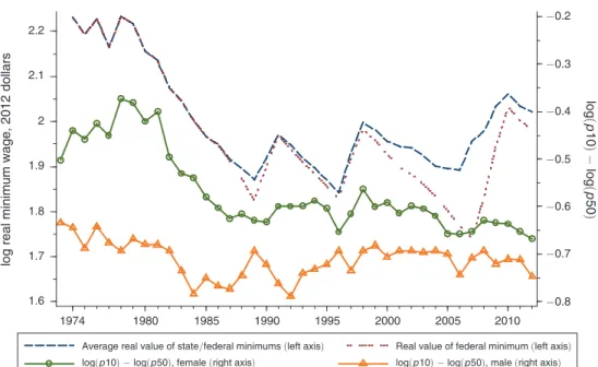
now over 20 years old. One possible reason is that while lower tail wage inequality

rose dramatically in the 1980s, it has not exhibited much of a trend since then (see

Figure 1, panel A_{). But this does not make the last 20 years irrelevant; these extra}

years encompass 3 increases in the federal minimum wage and a much larger num-ber of instances where state minimum wages exceeded the federal minimum wage. This additional variation will prove crucial in identifying the impact of minimum wages on wage inequality.

In this paper, we reassess the evidence on the minimum wage’s impact on US wage inequality with three specific objectives in mind. A first is to quantify how the numerous changes in state and federal minimum wages enacted in the two decades

since DFL _{(1996) and Lee’s (1999) data window closed have shaped the}

evolu-tion of inequality. A second is to understand why the minimum wage appears to

compress 50_{/10 inequality despite the fact that the minimum generally binds well}

below the tenth percentile. A third is to resolve what we see as a fundamental open

question in the literature that was raised by Lee _{(1999). This question is not whether}

the falling minimum wage contributed to rising inequality in the 1980s but whether underlying inequality was in fact rising at all absent the “unmasking” effect of the

falling minimum. Lee (1999) answered this question in the negative. And despite

the incompatibility of this conclusion with the rest of the literature, it has not drawn reanalysis.

We believe that the debate can now be cleanly resolved by combining a longer time window with a methodology that resolves first-order biases in existing liter-ature. We begin by showing why OLS estimates of the impact of the “effective minimum” on wage inequality are likely to be biased by measurement errors and transitory shocks that simultaneously affect both the dependent and independent

variables. Following the approach introduced by Durbin (1954), we purge these

biases by instrumenting the effective minimum wage with the legislated minimum

1 _{Using cross-region rather than cross-state variation in the “bindingness” of minimum wages, Teulings}₍₂₀₀₀

and 2003) reaches similar conclusions. Lemieux (2006) highlights the contribution of the minimum wage to the

evolution of residual inequality. Mishel, Bernstein, and Allegretto (2007, chapter 3) also offer an assessment of the

minimum wage’s effect on wage inequality.

(4)

Panel A. Minimum wages and log(p10) − log(p50)

Panel B. Minimum wages and log(p90) − log(p50)

−0.8 −0.7 −0.6 −0.5 −0.4 −0.3 −0.2 log (p 10 ) − log (p 50 ) 1.6 1.7 1.8 1.9 2 2.1 2.2

log real minimum wage, 2012 dollars

1974 1980 1985 1990 1995 2000 2005 2010

Average real value of state/federal minimums (left axis) log(p10) − log(p50), female (right axis)

Real value of federal minimum (left axis) log(p10) − log(p50), male (right axis)

0.5 0.6 0.7 0.8 0.9 1 1.1 log (p 90 ) − log (p 50 ) 1.6 1.7 1.8 1.9 2 2.1 2.2

log real minimum wage, 2012 dollars

1974 1980 1985 1990 1995 2000 2005 2010

Average real value of state/federal minimums (left axis) log(p90) − log(p50), female (right axis)

Real value of federal minimum (left axis) log(p90) − log(p50), male (right axis)

Figure 1. Trends in State and Federal Minimum Wages and Lower- and Upper-Tail Inequality

(5)

(and its square), an idea pursued by Card, Katz, and Krueger (1993) when studying

the impact of the minimum wage on employment _{(rather than inequality).}

Our instrumental variables analysis finds that the impact of the minimum wage on inequality is economically consequential but substantially smaller than that reported

by Lee (1999). The substantive difference comes from the estimation

methodol-ogy. Additional years of data and state-level legislative variation in the minimum

wage allow us to test (and reject) some of the identifying assumptions made by Lee

(1999). In most specifications, we conclude that the decline in the real value of the minimum wage explains 30 to 40 percent of the rise in lower tail wage inequality

in the 1980s. Holding the real minimum wage at its lowest _{(least binding) level}

throughout the 1980s, we estimate that female 50/10 inequality would have risen

by 11–15 log points, male inequality by approximately 1 log point, and pooled gen-der inequality by 7–8 log points. In other words, there was a substantial increase in underlying wage inequality in the 1980s.

In revisiting Lee’s estimates, we document that our instrumental variables strat-egy—which relies on variation in statutory minimum wages across states and over time—does not perform well when limited to data only from the 1980s period. This is because between 1979 and 1985, only one state aside from Alaska adopted a minimum wage in excess of the federal minimum; the ten additional state

adop-tions that occurred through 1989 all took place between 1986 and 1989 _(Table 1).

This provides insufficient variation to pin down a meaningful first-stage relationship between the legislated minimum wage and the effective minimum wage. By

extend-ing the estimation window to 1991 (as was also done by Lee 1999), we exploit the

substantial federal minimum wage increase that took place between 1990 and 1991 to tighten these estimates; extending the sample further to 2012 lends additional precision. We show that it would have been infeasible using data prior to 1991 to successfully estimate the effect of the minimum wage on the wage distribution. It is only with subsequent data on comovements in state wage distributions and the minimum wage that meaningful estimates can be obtained. Thus, the causal effect estimate that Lee sought to identify was only barely estimable within the confines of

his sample (though not with the methods used).

Our finding of a modest but meaningful effect of the minimum wage on 10_/50

inequality leaves open a second puzzle: why did the minimum wage have any effect at all? Between 1979 and 2012, there is no year in which more than 10 percent of male hours or aggregate hours were paid at or below the federal or applicable state

minimum wage _{(See Figure 2 and Tables 1A and 1B, columns 4 and 8), and only 5}

years in which more than 10 percent of female hours were at or below the minimum

wage. Thus, any impact of the minimum wage on 50_{/10 inequality among males or}

the pooled gender distribution must have arisen from spillovers, whereby the

min-imum wage must have raised the wages of workers earning above the minmin-imum.3

3 _{If there are disemployment effects, the minimum wage will have spillovers on the observed wage distribution}

even if no individual wage changes (see Lee 1999, for a discussion of this). The size of these spillovers will be

related to the size of the disemployment effect. Although the employment impact of the minimum wage remains a

contentious issue (see, for example, Card, Katz, and Krueger 1993; Card and Krueger 2000; Neumark and Wascher

2000; and more recently, see Allegretto, Dube, and Reich 2011 and Neumark, Salas, and Wascher 2014), most

(6)

Such spillovers are a potentially important and little understood effect of minimum wage laws, and we seek to understand why they arise.

Distinct from prior literature, we explore a novel interpretation of these spill-overs: measurement error. In particular, we assess whether the spillovers found in our samples, based on the Current Population Survey, may result from measurement

of a 25 percent rise in the federal minimum wage from $7.25 to $9.00 used a conventional labor demand approach but concluded job losses would represent less than 0.1 percent of employment. This would cause only a trivial spillover effect. In addition, we have explored how minimum wage related disemployment may affect our findings by limiting our sample to 25–64 year olds; because the studies that find disemployment effects generally find them concentrated among younger workers, focusing on older workers may limit the bias from disemployment. When we limit our sample in this way, we find that the effect of the minimum wage on lower tail inequality is somewhat smaller than for the full sample, consistent with a smaller fraction of the older sample earning at or below the min-imum. However, using our preferred specification, the contribution of changes in the minimum wage to changes in inequality is qualitatively similar regardless of the sample.

Table 1A—Summary Statistics for Bindingness of State and Federal Minimum Wages

A. Females States with > federal minimum (1) Minimum binding percentile (2) Maximum binding percentile (3) Share of hours at or below minimum (4) Average log( p10) − log( p50) (5) 1979 1 5.0 28.0 0.13 _−0.38 1980 1 6.0 24.0 0.13 −0.40 1981 1 5.0 24.0 0.13 _−0.41 1982 1 5.0 21.5 0.11 −0.48 1983 1 3.5 17.5 0.10 _−0.51 1984 1 2.5 15.5 0.09 −0.54 1985 2 2.0 14.5 0.08 _−0.56 1986 5 2.0 16.0 0.07 −0.59 1987 6 2.0 14.0 0.06 _−0.60 1988 10 2.0 12.5 0.06 −0.60 1989 12 1.0 12.5 0.05 _−0.61 1990 11 1.5 14.0 0.05 −0.58 1991 4 1.5 18.5 0.07 _−0.58 1992 7 2.0 14.0 0.07 −0.58 1993 7 2.5 11.0 0.06 _−0.59 1994 8 2.5 11.0 0.06 −0.61 1995 9 2.0 9.5 0.05 _−0.61 1996 11 1.5 12.5 0.05 −0.61 1997 10 2.5 14.5 0.06 _−0.60 1998 7 2.5 11.5 0.06 −0.58 1999 10 2.5 11.0 0.05 _−0.58 2000 10 2.0 9.5 0.05 −0.59 2001 10 2.0 9.0 0.05 _−0.59 2002 11 1.5 9.0 0.04 −0.60 2003 11 1.5 9.0 0.04 _−0.61 2004 12 1.5 7.5 0.04 −0.63 2005 15 1.5 8.5 0.04 _−0.64 2006 19 1.5 9.5 0.04 −0.64 2007 30 1.5 10.0 0.05 _−0.63 2008 31 2.0 13.0 0.06 −0.64 2009 26 2.5 10.5 0.06 _−0.64 2010 15 3.5 9.5 0.06 −0.64 2011 19 3.0 10.5 0.06 _−0.65 2012 19 3.0 9.5 0.06 −0.66

(7)

artifacts. This can occur if a fraction of minimum wage workers report their wages inaccurately, leading to a hump in the wage distribution centered on the minimum

wage rather than _{(or in addition to) a spike at the minimum. After bounding the}

potential magnitude of these measurement errors, we are unable to reject the

hypoth-esis that the apparent spillover from the minimum wage to higher _(noncovered)

per-centiles is spurious. That is, while the spillovers are present in the data, they may not be present in the distribution of wages actually paid. These results do not rule

Table 1B—Summary Statistics for Bindingness of State and Federal Minimum Wages

B. Males C. Males and females, pooled

Minimum binding percentile (1) Maximum binding percentile (2) Share of hours at or below minimum (3) Average log(10) − log(50) (4) Minimum binding percentile (5) Maximum binding percentile (6) Share of hours at or below minimum (7) Average log( p10) − log( p50) (8) 1979 2.0 10.5 0.05 −0.64 3.5 17.0 0.08 −0.58 1980 2.5 10.0 0.06 _−0.65 4.0 15.5 0.09 _−0.59 1981 1.5 9.0 0.06 −0.68 2.5 14.5 0.09 −0.60 1982 2.0 8.0 0.05 _−0.71 3.5 12.5 0.07 _−0.63 1983 2.0 8.0 0.05 −0.73 3.0 11.5 0.07 −0.65 1984 1.5 7.5 0.04 _−0.73 2.0 10.5 0.06 _−0.67 1985 1.0 6.5 0.04 −0.74 1.5 9.5 0.06 −0.69 1986 1.0 6.5 0.03 _−0.74 1.5 10.0 0.05 _−0.70 1987 1.0 6.0 0.03 −0.73 1.5 9.0 0.04 −0.70 1988 1.0 6.0 0.03 _−0.72 1.5 8.0 0.04 _−0.69 1989 1.0 5.0 0.03 −0.72 1.0 7.0 0.04 −0.68 1990 0.5 6.0 0.03 _−0.72 0.5 9.0 0.04 _−0.67 1991 0.5 9.0 0.04 −0.71 1.0 12.5 0.05 −0.67 1992 1.0 6.5 0.04 _−0.72 1.5 9.5 0.05 _−0.67 1993 1.0 5.0 0.03 −0.73 1.5 7.5 0.04 −0.68 1994 1.0 4.5 0.03 _−0.71 2.0 7.5 0.04 _−0.69 1995 0.5 4.5 0.03 −0.71 1.5 6.0 0.04 −0.68 1996 1.0 7.0 0.03 _−0.71 1.5 9.0 0.04 _−0.67 1997 1.0 7.5 0.04 −0.69 1.5 10.0 0.05 −0.66 1998 1.0 7.0 0.04 _−0.69 2.0 8.0 0.05 _−0.65 1999 1.0 5.5 0.03 −0.69 2.0 7.0 0.04 −0.65 2000 1.0 6.0 0.03 _−0.68 1.5 7.5 0.04 _−0.65 2001 0.5 5.5 0.03 −0.68 1.5 7.0 0.04 −0.66 2002 1.0 6.0 0.03 _−0.69 1.5 7.5 0.03 _−0.65 2003 0.5 5.0 0.03 −0.69 1.5 6.5 0.03 −0.66 2004 1.0 5.0 0.03 _−0.70 1.5 6.0 0.03 _−0.68 2005 1.0 5.0 0.02 −0.71 1.5 6.5 0.03 −0.68 2006 0.5 6.0 0.02 _−0.70 1.0 7.5 0.03 _−0.68 2007 0.5 6.0 0.03 −0.70 1.5 7.5 0.04 −0.68 2008 1.0 6.5 0.04 _−0.71 1.0 8.5 0.04 _−0.69 2009 1.0 6.0 0.04 −0.74 2.0 8.0 0.05 −0.71 2010 2.0 6.5 0.04 _−0.73 3.0 7.5 0.05 _−0.70 2011 1.5 8.0 0.04 −0.72 2.5 9.0 0.05 −0.69 2012 1.5 7.0 0.04 _−0.74 2.0 8.0 0.05 _−0.71

Notes: Column 1 in Table 1A displays the number of states with a minimum that exceeds the federal minimum for at least six months of the year. Columns 2 and 3 of Table 1A, and columns 1, 2, 5, and 6 of Table 1B display

esti-mates of the lowest and highest percentile at which the minimum wage binds across states (DC is excluded). The

binding percentile is estimated as the highest percentile in the annual distribution of wages at which the minimum

wage binds (rounded to the nearest half of a percentile), where the annual distribution includes only those months

for which the minimum wage was equal to its modal value for the year. Column 4 of Table 1A and columns 3 and 7 of Table 1B display the share of hours worked for wages at or below the minimum wage. Column 5 of Table 1A

and columns 4 and 8 of Table 1B display the weighted average value of the log( p10) − log( p50) for the male or

(8)

out the possibility of true spillovers. But they underscore that spillovers estimated with conventional household survey data sources must be treated with caution since they cannot necessarily be distinguished from measurement artifacts with available precision.

The paper proceeds as follows. Section I discusses data and sources of identifica-tion. Section II presents the measurement framework and estimates a set of causal

effects estimates models that, like Lee (1999), explicitly account for the bite of

the minimum wage in estimating its effect on the wage distribution. We compare parameterized OLS and 2SLS models and document the pitfalls that arise in the OLS estimation. Section III uses point estimates from the main regression models to calculate counterfactual changes in wage inequality, holding the real minimum wage constant. Section IV analyzes the extent to which apparent spillovers may be due to measurement error. The final section concludes.

I. Changes in the Federal Minimum Wage and Variation in State Minimum Wages

In July of 2007, the real value of the US federal minimum wage fell to its lowest point in over three decades, reflecting a nearly continuous decline from a 1979 high point, including two decade-long spans in which the minimum wage remained fixed in nominal terms—1981 through 1990, and 1997 through 2007. Perhaps responding to federal inaction, numerous states have over the past two decades legislated state minimum wages that exceed the federal level. At the end of the 1980s, 12 states’ minimum wages exceeded the federal level; by 2008, this number had reached

31 _{(subsequently reduced to 15 by the 2009 federal minimum wage increase).}4

4 _{Table 1 assigns each state the minimum wage that was in effect for the largest number of months in a calendar}

year. Because the 2009 federal minimum wage increase took effect in late July, it is not coded as exceeding most state minimums until 2010.

0 0.02 0.04 0.06 0.08 0.1 0.12 0.14

Share at or below the minimum

1979 1985 1990 1995 2000 2005 2010

Female Male/female pooled

Male

Figure 2. Share of Hours at or Below the Minimum Wage

Notes: The figure plots estimates of the share of hours worked for reported wages equal to or less than the applicable state or federal minimum wage, corresponding with data from columns 4 and 8 of Tables 1A and 1B.

(9)

Consequently, the real value of the minimum wage applicable to the average worker in 2007 was not much lower than in 1997, and was significantly higher than if states had not enacted their own minimum wages. Moreover, the post-2007 federal increases brought the minimum wage faced by the average worker up to a real level not seen since the mid-1980s. An online Appendix table illustrates the extent of state minimum wage variation between 1979 and 2012.

These differences in legislated minimum wages across states and over time are one of two sources of variation that we use to identify the impact of the minimum wage on the wage distribution. The second source of variation we use, following Lee (1999), is variation in the “bindingness” of the minimum wage, stemming from the observation that a given legislated minimum wage should have a larger effect on the shape of the wage distribution in a state with a lower wage level. Table 1 provides examples. In each year, there is significant variation in the percentile of the state wage distribution where the state or federal minimum wage “binds.” For instance, in 1979 the minimum wage bound at the twelfth percentile of the female wage dis-tribution for the median state, but it bound at the fifth percentile in Alaska and the twenty-eighth percentile in Mississippi. This variation in the bite or bindingness of the minimum wage was due mainly to cross-state differences in wage levels in 1979, since only Alaska had a state minimum wage that exceeded the federal minimum. In later years, particularly during the 2000s, this variation was also due to differences in the value of state minimum wages.

A. Sample and Variable construction

Our analysis uses the percentiles of states’ annual wage distributions as the primary outcomes of interest. We form these samples by pooling all individual responses from the Current Population Survey Merged Outgoing Rotation Group (CPS MORG) for each year. We use the reported hourly wage for those who report being paid by the hour. Otherwise we calculate the hourly wage as weekly earnings divided by hours worked in the prior week. We limit the sample to individuals age 18 through 64, and we multiply top-coded values by 1.5. We exclude self-employed individuals and those with wages imputed by the BLS. To reduce the influence of outliers, we Winsorize the top two percentiles of the wage distribution in each state,

year, and sex grouping _{(male, female, or pooled) by assigning the ninety-seventh}

percentile value to the ninety-eighth and ninety-ninth percentiles. Using these indi-vidual wage data, we calculate all percentiles of state wage distributions by sex for 1979–2012, weighting individual observations by their CPS sampling weight

multi-plied by their weekly hours worked.5_{For more details on our data construction, see}

the data Appendix.

Our primary analysis is performed at the state-year level, but minimum wages often change part way through the year. We address this issue by assigning the value of the minimum wage that was in effect for the longest time throughout the calendar

5 _{Following the approach introduced by DFL}_{(1996), now used widely in the wage inequality literature, we}

define percentiles based on the distribution of paid hours, thus giving equal weight to each paid hour worked. Our estimates are essentially unchanged if we weight by workers rather by worker hours.

(10)

year in a state and year. For those states and years in which more than one minimum wage was in effect for six months in the year, the maximum of the two is used. We have alternatively assigned the maximum of the minimum wage within a year as the applicable minimum wage. This leaves our conclusions unchanged.

II. Reduced Form Estimation of Minimum Wage Effects on the Wage Distribution

A. General Specification and oLS Estimates

The general model we estimate for the evolution of inequality at any point in the

wage distribution (the difference between the log wage at the pth percentile and the

log of the median_{) for state s in year t is of the form:}

rep-resented by _ε_stσ_{( p) , which we assume to be independent of the state and year effects} and trends. Although our state effects and trends are likely to control for much of the economic fluctuations at state level, we also experimented with including the state-level unemployment rate as a control variable. This has virtually no impact on the

estimated coefficients in equation _{(1) for any of our samples.}

In equation (1), w _stm _{is the log minimum wage for that state-year. We follow Lee}

(1999) in both defining the bindingness of the minimum wage to be the log

differ-ence between the minimum wage and the median (Lee refers to this as the effective

minimum_{) and in modeling the impact of the minimum wage to be quadratic. The}

quadratic term is important to capture the idea that a change in the minimum wage

is likely to have more impact on the wage distribution where it is more binding.6_By

differentiating (1) we have that the predicted impact of a change in the minimum

wage on a percentile is given by _β₁

(

_p

)

_{+ 2 β}₂

(

_p

)

_[_w_stm_{− w}

st

(

50

)

] . Inspection of this

expression shows how our specification captures the idea that the minimum wage will have a larger effect when it is high relative to the median.

Our preferred strategy for estimating (1) is to include state fixed effects and trends

and to instrument the minimum wage.7_{But we start by presenting OLS estimates}

6 _{In this formulation, a more binding minimum wage is a minimum wage that is closer to the median, resulting in}

a higher (less negative) effective minimum wage. Since the log wage distribution has greater mass toward its center

than at its tail, a 1 log point rise in the minimum wage affects a larger fraction of wages when the minimum lies at the fortieth percentile of the distribution than when it lies at the first percentile.

7 _{Our primary specification does not control for other state-level controls. When we include state-year}

unem-ployment rates to proxy for heterogeneous shocks to a state’s labor market, however, the coefficients on the mini-mum wage variables are essentially unchanged.

(11)

of _(1).8_{Column 1 of Tables 2A and 2B reports estimates of this specification. We}

report the marginal effects of the effective minimum for selected percentiles when

8 _{Strictly speaking our OLS estimates are weighted least squares and our IV estimates weighted two-stage least}

squares.

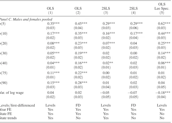
Table 2A—OLS and 2SLS Relationship between log( p) − log( p50) and

log_{(min. wage) − log( p50), for Select Percentiles of}

Given Wage Distribution, 1979–2012 OLS (1) OLS(2) 2SLS(3) 2SLS(4) OLS Lee Spec. (5) panel A. Females p(5) 0.44*** 0.54*** 0.32*** 0.39*** 0.63*** (0.03) (0.05) (0.04) (0.05) (0.04) p(10) 0.27*** 0.46*** 0.22*** 0.17*** 0.52*** (0.03) (0.03) (0.05) (0.03) (0.03) p(20) 0.12*** 0.29*** 0.10** 0.07** 0.29*** (0.03) (0.03) (0.05) (0.03) (0.03) p(30) 0.07*** 0.23*** 0.02 0.04 0.15*** (0.01) (0.02) (0.02) (0.03) (0.02) p(40) 0.04** 0.17*** 0.00 0.03 0.06*** (0.02) (0.02) (0.03) (0.03) (0.01) p(75) 0.09*** 0.23*** −0.03 0.00 −0.05** (0.02) (0.03) (0.02) (0.03) (0.02) p(90) 0.15*** 0.34*** _−0.02 0.04 _−0.04 (0.03) (0.03) (0.04) (0.04) (0.04)

Var. of log wage 0.07 0.04 −0.02 −0.09 −0.20***

(0.04) (0.05) (0.08) (0.07) (0.03) panel B. males p(5) 0.25*** 0.43*** 0.19*** 0.16*** 0.55*** (0.03) (0.03) (0.02) (0.04) (0.04) p(10) 0.12*** 0.34*** 0.05 0.05* 0.38*** (0.04) (0.03) (0.04) (0.03) (0.04) p(20) 0.06** 0.23*** 0.02 0.02 0.21*** (0.03) (0.02) (0.02) (0.03) (0.03) p(30) 0.04 0.19*** 0.02 0.00 0.09*** (0.02) (0.02) (0.02) (0.03) (0.02) p(40) 0.06*** 0.15*** 0.05* 0.02 0.03*** (0.01) (0.02) (0.02) (0.04) (0.01) p(75) 0.14*** 0.23*** 0.00 0.02 0.09** (0.02) (0.02) (0.02) (0.02) (0.04) p(90) 0.16*** 0.30*** 0.03 0.04 0.14** (0.03) (0.03) (0.03) (0.04) (0.07)

Var. of log wage 0.03 0.01 −0.07 −0.06 −0.12**

(0.03) (0.05) (0.05) (0.07) (0.05)

Levels/first-differenced Levels FD Levels FD Levels

Year FE Yes Yes Yes Yes Yes

State FE Yes Yes Yes Yes No

State trends Yes No Yes No No

Notes: See text at bottom of Table 2B.

*** Significant at the 1 percent level.

** Significant at the 5 percent level.

(12)

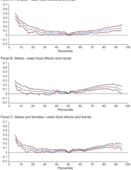
estimated at the weighted average of the effective minimum over all states and all years between 1979 and 2012. In the final row we also report an estimate of the effect on the variance, though the upper tail will heavily influence this estimate. Figure 3 provides a graphical representation of these estimated marginal effects for

all percentiles. In all three samples _{(males, females, pooled), there is a significant}

estimated effect of the minimum wage on the lower tail, but, rather worryingly, there is also a large positive relationship between the effective minimum wage and upper

tail inequality. This suggests there is some bias in these estimates. This problem also occurs when we estimate the model with first-differences in column 2.

Table 2B—OLS and 2SLS Relationship between log( p) − log( p50) and

log_{(min. wage) − log( p50), for Select Percentiles}

of Pooled Wage Distribution, 1979–2012 OLS

(1) OLS(2) 2SLS(3) 2SLS(4)

OLS Lee Spec.

(5)

panel c. males and females pooled

p(5) 0.35*** 0.45*** 0.29*** 0.29*** 0.62*** (0.03) (0.04) (0.03) (0.06) (0.03) p(10) 0.17*** 0.35*** 0.16*** 0.17*** 0.44*** (0.02) (0.03) (0.02) (0.04) (0.03) p(20) 0.08*** 0.23*** 0.07*** 0.04 0.25*** (0.02) (0.03) (0.02) (0.03) (0.03) p(30) 0.05*** 0.19*** 0.02 0.00 0.14*** (0.02) (0.02) (0.02) (0.02) (0.02) p(40) 0.04*** 0.16*** 0.02** 0.02 0.06*** (0.01) (0.02) (0.01) (0.03) (0.01) p(75) 0.11*** 0.22*** 0.00 0.01 0.01 (0.01) (0.02) (0.02) (0.02) (0.02) p(90) 0.15*** 0.28*** 0.01 0.02 0.04 (0.03) (0.03) (0.04) (0.03) (0.05)

Var. of log wage 0.04 0.02 −0.05 −0.07 −0.18***

(0.02) (0.03) (0.05) (0.05) (0.04)

Levels/first-differenced Levels FD Levels FD Levels

Year FE Yes Yes Yes Yes Yes

State FE Yes Yes Yes Yes No

State trends Yes No Yes No No

Notes: N = 1,700 for levels estimation, N = 1,650 for first-differenced estimation. Sample period is 1979–2012.

For all but the last row, the dependent variable is log( p) − log( p50), where p is the indicated percentile. For

the last row, the dependent variable is the variance of log wage. Estimates are the marginal effects of log(min.

wage) − log( p50), evaluated at its hours-weighted average across states and years. The last row are estimates of

the marginal effects of log(min. wage) − log( p50), evaluated at its hours-weighted average across states and years.

Standard errors clustered at the state level are in parentheses. Regressions are weighted by the sum of individu-als’ reported weekly hours worked multiplied by CPS sampling weights. For 2SLS specifications, the effective minimum and its square are instrumented by the log of the minimum, the square of the log minimum, and the log minimum interacted with the average real log median for the state over the sample. For the first-differenced speci-fication, the instruments are first-differenced equivalents.

*** Significant at the 1 percent level. ** Significant at the 5 percent level.

(13)

In discussing the possible causes of bias in estimates, it is helpful to consider the following model for the median log wage for state s in year t:

(2) w st

(

50

)

= μ s0 + μ s1 × tim e t + γ tμ + ε stμ .

Here, the median wage for the state is a function of a state effect, μ _s0 ; a state

trend, _μ_s₁_{; a common year effect, γ}_tμ_{; and a transitory effect, ε}_stμ_{. With this setup, OLS} estimation of (1) will be biased if cov

(

ε _stμ , ε _stσ ( p)

)

is nonzero because the median is used in the construction of the effective minimum; that is, transitory fluctuations

Panel A. Females—state fixed effects and trends

Panel B. Males—state fixed effects and trends

Panel C. Males and females—state fixed effects and trends

−0.2 −0.1 0 0.1 0.2 0.3 0.4 0.5 0.6 0.7 0 10 20 30 40 50 60 70 80 90 100 Percentile 0 10 20 30 40 50 60 70 80 90 100 Percentile 0 10 20 30 40 50 60 70 80 90 100 Percentile −0.2 −0.1 0.1 0.2 0.3 0.4 0.5 0.6 0.7 0 −0.2 −0.1 0.1 0.2 0.3 0.4 0.5 0.6 0.7 0

Figure 3. OLS Estimates of the Relationship between log( p) – log( p50) and log(min) – log( p50)

and Its Square, 1979–2012

Notes: Estimates are the marginal effects of log(min. wage) – log( p50), evaluated at the hours-weighted average

of log(min. wage) – log( p50) across states and years. Observations are state-year observations. Ninety-five percent

introduced by Durbin (1954). We instrument the observed effective minimum and

its square using an instrument set that consists of: _{(i) the log of the real statutory}

minimum wage, (ii) the square of the log of the real minimum wage, and (iii) the

interaction between the log minimum wage and average log median real wage for

the state over the sample period. In this IV specification, identification in (1) for

the linear term in the effective minimum wage comes entirely from the variation in the statutory minimum wage, and identification for the quadratic term comes from the inclusion of the square of the log statutory minimum wage and the interaction term.9_{As there are always time effects included in our estimation, all the identifying}

variation in the statutory minimum comes from the state-specific minimum wages,

which we assume to be exogenous to state wage levels of inequality.10_{Our second}

instrument is the square of the predicted value for the effective minimum from the

regression outlined above, and relies on the same identifying assumptions

(exoge-neity of the statutory minimum wage_).

Column 3 of Tables 2A and 2B report the estimates when we instrument the effective minimum in the way we have described. The first-stages for these regres-sions are reported in Appendix Table A1. For all samples, the three instruments are

9 _{To see why the interaction is important to include, expand the square of the effective minimum wage,}

log(min) − log( p50), which yields three terms, one of which is the interaction of log(min) and log( p50). We

have also tried replacing the square and interaction terms with the square of the predicted value for the effective minimum, where the predicted value is derived from a regression of the effective minimum on the log statutory

min-imum, state and time fixed effects, and state trends (similar to an approach suggested by Wooldridge 2002; section

9.5.2). 2SLS results using this alternative instrument are virtually identical to the strategy outlined in the main text.

In general, using the statutory minimum as an instrument is similar in spirit to the approach taken by Card, Katz,

and Krueger (1993) in their analysis of the employment effects of the minimum wage.

10 _{We follow almost all of the existing literature and assume the state level minimum wages are exogenous to}

other factors affecting the state-level wage distribution once we have controlled for state fixed effects and trends. A priori, any bias is unclear, e.g., rising inequality might generate a demand for higher minimum wages as might economic conditions favorable to minimum wage workers. The long lags in the political process surrounding rises in the minimum wages makes it unlikely that there is much response to contemporaneous economic conditions.

(15)

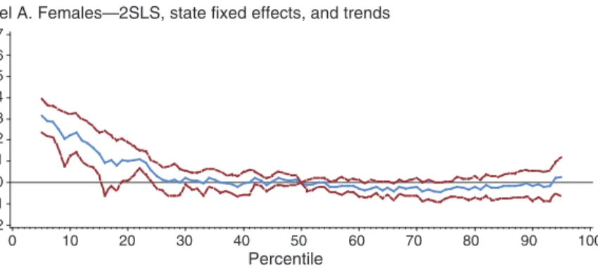
jointly highly significant and pass standard diagnostic tests for weak instruments (e.g., Stock, Wright, and Yogo 2002). Compared to column 1, the estimated impacts of the minimum wage in the lower tail are reduced, especially above the tenth per-centile. This is consistent with what we have argued is the most plausible direction of bias in the OLS estimate in column 1. And, for all three samples, the estimated effect in the upper tail is now small and insignificantly different from zero, again

consistent with the IV strategy reducing bias in the predicted direction.11

For robustness, we also estimate these models in first differences. Column 4 shows the results from first-differenced regressions that include state and year fixed effects, instrumenting the endogenous differenced variables using differenced

ana-logues to the instruments described above.12_{Figure 4A shows the results for all}

percentiles from the level IV specifications; Figure 4B shows the results from the first-differenced IV specifications. Qualitatively, the first-differenced regressions are quite similar to the levels regressions, although they imply slightly larger effects of the minimum wage at the bottom of the wage distribution.

Our 2SLS estimates find that the minimum wage affects lower tail inequality up through the twenty-fifth percentile for women, up through the tenth percentile for men, and up through approximately the fifteenth percentile for the pooled wage

distribution. A 10 log point increase in the effective minimum wage reduces 50/10

inequality by approximately 2 log points for women, by no more than 0.5 log points for men, and by roughly 1.5 log points for the pooled distribution. These estimates are less than half as large as those found by the baseline OLS specification, and are

considerably smaller than those reported by Lee (1999). What accounts for this

qualitative difference in findings? The dissimilarity could stem either from differ-ences in specification and estimation or from the additional years of data available for our analysis. We consider both factors in turn, and show that the first—differ-ences in specification and estimation—is fundamental.

B. reconciling with Literature: methods or Time period?

Lee (1999) estimates equation (1) by OLS and his preferred specification excludes

the state fixed effects and trends that we have included.13_{Column 5 of Tables 2A}

and 2B, and Figure 5, shows what happens when we estimate this model on our lon-ger sample period. Similar to Lee, we find large and statistically significant effects of the minimum wage on the lower percentiles of the wage distribution that extend throughout all percentiles below the median for the male, female, and pooled wage distributions, and are much larger than the effects in our preferred specifications. Also note that, with the exception of the male estimates, the upper tail “effects” are small and insignificantly different from zero, which might be considered a necessary

11 _{These findings are essentially unchanged if we use higher order state time trends.}

12 _{The instruments for the first-differenced analogue are}_{Δ w}

stm and Δ ( w stm − w ̃ (50) st ) 2 , where Δ w stm represents

the annual change in the log of the legislated minimum wage, and Δ ( w stm − w ̃ ̃ (50)st ) 2 represents the change in the

square of the predicted value for the effective minimum wage.

13 _{We include time effects in all of our estimation, as does Lee}_{(1999). We estimate the model separately for}

(16)

condition for the results to be credible estimates of the impact of the minimum wage on wage inequality at any point in the distribution.

These estimates are likely to suffer from serious biases, however. If state fixed

effects and trends are omitted from the specification of (1), estimates of minimum

wage effects on wage inequality will be biased if

(

_σ_s₀_{( p), σ}_s₁_{( p)}

)

_{is correlated with}

(

μ s0 , μ s1

)

, that is, state log median wage levels and latent state log wage inequality

are correlated. Lee _{(1999) is very clear that his specification relies on the}

assump-tion of a zero correlaassump-tion between the level of median wages and inequality. This assumption can be tested if one has a measure of inequality that is unlikely to be

Panel C. Males and females—2SLS, state fixed effects, and trends

0 10 20 30 40 50 60 70 80 90 100 Percentile −0.2 −0.1 0.1 0.2 0.3 0.4 0.5 0.6 0.7 0

Panel A. Females—2SLS, state fixed effects, and trends

Panel B. Males—2SLS, state fixed effects, and trends

−0.2 −0.1 0 0.1 0.2 0.3 0.4 0.5 0.6 0.7 0 10 20 30 40 50 60 70 80 90 100 Percentile 0 10 20 30 40 50 60 70 80 90 100 Percentile −0.2 −0.1 0.1 0.2 0.3 0.4 0.5 0.6 0.7 0

Figure 4A. 2SLS Estimates of the Relationship between log( p) – log( p50) and log(min) – log( p50)

and Its Square, 1979–2012

of log_{(min. wage) – log( p50) across states and years. Observations are state-year observations. Ninety-five percent}

(17)

affected by the level of the minimum wage. For this purpose we use 60_/40 inequal-ity, that is, the difference in the log of the sixtieth and fortieth percentiles. Given that the minimum wage never binds very far above the tenth percentile of the wage dis-tribution over our sample period, we feel comfortable assuming that the minimum wage has no impact on percentiles 40 through 60. Under this maintained hypothesis,

60/40 inequality serves as a valid proxy for the underlying inequality of a state’s

wage distribution.

To assess whether either the level or trend of state latent inequality is correlated with average state wage levels or their trends, we estimate state-level regressions

Panel C. Males and females—2SLS, first-differenced, and state fixed effects

0 10 20 30 40 50 60 70 80 90 100 Percentile −0.2 −0.1 0.1 0.2 0.3 0.4 0.5 0.6 0.7 0

Panel A. Females—2SLS, first-differenced, and state fixed effects

Panel B. Males—2SLS, first-differenced, and state fixed effects

−0.2 −0.1 0 0.1 0.2 0.3 0.4 0.5 0.6 0.7 0 10 20 30 40 50 60 70 80 90 100 Percentile 0 10 20 30 40 50 60 70 80 90 100 Percentile −0.2 −0.1 0.1 0.2 0.3 0.4 0.5 0.6 0.7 0

Figure 4B. 2SLS Estimates of the Relationship between log( p) – log( p50) and log(min) – log( p50)

in First-Differences, 1979–2012

of log(min. wage) – log( p50) across states and years. Observations are state-year observations. Ninety-five percent

(18)

of average 60_{/40 inequality and estimated trends in 60/40 inequality on average} median wages and trends in median wages. Figures 6A and 6B depict scatter plots of these regressions, with regression results reported in Appendix Table A1. Figure 6A

depicts the cross-state relationship between the average log( p60)–log( p40) and the

average log_{( p50) for each of our three samples. Figure 6B depicts the cross-state}

relationship between the trends in the two measures. In all cases but the male trends plot _{(panel B of Figure 6B), there is a strong, positive visual relationship between the} two—and, even for the male trend scatter, there is, in fact, a statistically significant

positive relationship between the trends in the log_{( p60)–log( p40) and log( p50).}

Panel C. Males and females—OLS, no state fixed effects

0 10 20 30 40 50 60 70 80 90 100 Percentile −0.1 0.1 0.2 0.3 0.4 0.5 0.6 0.7 0

Panel A. Females—OLS, no state fixed effects

Panel B. Males—OLS, no state fixed effects

−0.2 −0.1 0 0.1 0.2 0.3 0.4 0.5 0.6 0.7 0 10 20 30 40 50 60 70 80 90 100 Percentile 0 10 20 30 40 50 60 70 80 90 100 Percentile −0.2 −0.1 0.1 0.2 0.3 0.4 0.5 0.6 0.7 0 −0.2

Figure 5. 2SLS Estimates of the Relationship between log( p) – log( p50) and log(min) – log( p50)

and Its Square Using Lee _{(1999) Specification, 1979–2012}

of log_{(min. wage) – log( p50) across states and years. Observations are state-year observations. Ninety-five percent}

(19)

The finding of a positive correlation between underlying inequality and the state median implies there is likely to be omitted variable bias from the exclusion of state fixed effects and trends—specifically, an upward bias to the estimated minimum wage effect in the lower tail and, simultaneously, a downward bias in the upper tail. To see

why, note that higher wage states have lower _{(more negative) effective minimum}

wages (defined as the log gap between the legislated minimum and the state median),

and the results from Table 2 imply that these states also have higher levels of latent

M E N H V T M A R I CT N Y NJ PA OH IN ILM I W I M N I A M O N D S D N E KS DE M D V A W V N C S C GA FL K Y TN A L M S A R L A OK TX MT I D W Y C O N M AZ U T N V W A O R C A HI 0.2 0.25 0.3 0.35 Mean log (p 60 ) − log (p 40 ), 1979–2012 1.7 1.8 1.9 2 2.1 2.2 2.3 Mean log(p50), 1979–2012

Panel C. Males and females

M E N H VT M A R I CT N Y N J P A OH IN IL M I W I MN IA M O ND S D NE K S D E M D V A W V NC SC G A FL K Y TN AL MS AR L A OK TX M T ID W Y C O NM A Z U T N V W A OR CA H I 1.8 1.9 2 2.1 2.2 2.3 2.4 Mean log(p50), 1979–2012 0.2 0.25 0.3 0.35 Mean log (p 60 ) − log (p 40 ), 1979–2012 Panel B. Males M E N H VT M A RI C T N Y NJ PA OH IN IL MI W I M N IAM O N D S D N E K S D E M D V A W V N C SC G A FL KY TN A L M S A R LA OK TX M T ID W Y C O NM A Z U T N V W A OR C A H I 1.5 1.6 1.7 1.8 1.9 2 2.1 Mean log(p50), 1979–2012 0.2 0.25 0.3 0.35 Mean log (p 60 ) − log (p 40 ), 1979–2012 Panel A. Females

Figure 6A. OLS Estimates of the Relationship between Mean log( p60) – log( p40)

and Mean log( p50), 1979–2012

Notes: Estimates correspond with regressions from Appendix Table A2. The figures show the cross-state

relation-ship between the average log( p60) – log( p40) and log( p50) between 1979 and 2012. Alaska, which tends to be

an outlier, is dropped for visual clarity, though this does not materially affect the slope of the line (Appendix Table

(20)

inequality; thus they will have a more negative value of the left-hand side variable

in our main estimating equation _{(1) for percentiles below the median, and a more}

positive value for percentiles above the median. Since the state median enters the right-hand side expression for the effective minimum wage with a negative sign, esti-mates of the relationship between the effective minimum and wage inequality will be

upward-biased in the lower tail and downward-biased in the upper tail.

Combined with our discussion above on potential biases stemming from the

correlation between the transitory error components on both sides of equation _(1),

M E NH VT M A R I C T NY N J P A O H IN IL M I W I M N I A M O N D SD N E K S D E MD VA W V N C SC GA F L K Y TN AL M S AR LA OK TX M T ID W Y C O N MU T A Z NV W A O R C A H I −0.005 −0.0025 0 0.0025 0.005 0 0.005 0.01 0.015 Trend log(p50), 1979–2012 M E NH VT M A RI CT N Y N J PA OH IN I L M I W I M N IA M O ND S D N E K S DE M D VA W V NC S C GA FL K Y TN A L M S AR L A OKTX M T I D W Y C O N M AZ U T N V W A OR CA H I −0.006 −0.001 0.004 0.009 Trend log(p50), 1979–2012 M E _{V T} NH MA R I C T NY N J P A OH I N IL M I W I M N I A M O N D _SD N E K S D E M D V A W V NC SC _GA FL K Y TN AL MS A R L A OK TX M T ID W Y C O N M A Z U T N V W A O R CA HI −0.003 0.002 0.007 0.012 Trend log(p50), 1979–2012 Trend log (p 60 ) − log (p 40 ), 1979–2012

Panel C. Males and females

Trend log (p 60 ) − log (p 40 ), 1979–2012 Panel B. Males Trend log (p 60 ) − log (p 40 ), 1979–2012 Panel A. Females −0.005 −0.0025 0 0.0025 0.005 −0.005 −0.0025 0 0.0025 0.005

Figure 6B. OLS Estimates of the Relationship between Trend log( p60) – log( p40)

and Trend log( p50), 1979–2012

Notes: Estimates correspond with regressions from Appendix Table A2. The figures show the cross-state

relation-ship between the trend in log( p60) − log( p40) and the trend in log( p50) between 1979 and 2012. Alaska, which

tends to be an outlier, is dropped for visual clarity, though this does not materially affect the slope of the line (Appendix Table A2 includes Alaska).

(21)

which leads to an upward bias on the coefficient on the effective minimum wage in both lower and upper tails, we infer that these two sources of bias reinforce each other in the lower tail, likely leading to an overestimate of the impact of the mini-mum wage on lower tail inequality. Simultaneously, they have countervailing effects on the upper tail. Thus, our finding in the fifth column of Table 2 of a relatively weak

relationship between the effective minimum wage and upper tail inequality _{(for the}

female and pooled samples) may arise because these two countervailing sources of

bias largely offset one another for upper tail estimates. But since these biases are reinforcing in the lower tail of the distribution, the absence of an upper tail correla-tion is not sufficient evidence for the absence of lower tail bias, implying that Lee’s (1999) preferred specification may suffer from upward bias.

The original work assessing the impact of the minimum wage on rising US wage

inequality—including DFL (1996), Lee (1999), and Teulings (2000, 2003)—used

data from 1979 through the late 1980s or early 1990s. Our primary estimates exploit an additional 21 years of data. Does this longer sample frame make a substan-tive difference? Figure 7 answers this question by plotting estimates of marginal

Table 3—Actual and Counterfactual Changes in log_{( p50/10) between Selected Years:}

Changes in log Points (100 × log Change)

Observed change

(1)

2SLS counterfactuals OLS counterfactuals

Levels FE 1979–2012 (2) First diffs 1979–2012 (3) _{Levels, No FE} 1979–2012 (4) 1979–1991(5) panel A. 1979–1989 Females 24.6 11.3*** 15.1*** 2.9 4.3*** (3.7) (1.8) (2.0) (1.3) Males 2.5 1.2 1.4 _−6.5*** _−5.3*** (1.4) (0.9) (1.4) (1.6) Pooled 11.8 6.7*** 8.1*** −1.2 0.0 (1.8) (0.8) (1.3) (1.2) panel B. 1979–2012 Females 28.5 14.8*** 18.6*** 6.4*** 7.4*** (3.7) (1.8) (1.9) (1.3) Males 7.9 7.0*** 7.1*** 3.1*** 3.6*** (1.0) (0.7) (1.0) (0.9) Pooled 11.4 6.9*** 7.9*** 1.1 1.8** (1.5) (0.7) (1.2) (0.8)

Notes: Estimates represent changes in actual and counterfactual log( p50) − log( p10) between 1979 and 1989,

and 1979 and 2012, measured in log points (100 × log change). Counterfactual wage changes in panel A

repre-sent counterfactual changes in the 50/10 had the effective minimum wage in 1979 equaled the effective minimum

wage in 1989 for each state. Counterfactual wage changes in panel B represent changes had the effective minima in

1979 and 2012 equaled the effective minimum in 1989. The 2SLS counterfactuals (using point estimates from the

1979–2012 period) are formed using coefficients from estimations reported in columns 3 and 4 of Tables 2A and

2B. The OLS counterfactual estimates (using point estimates from the 1979–2012 period) are formed using

coeffi-cients from estimations reported in column 5 of Table 2. Counterfactuals using point estimates from the 1979–1991 period are formed using coefficients from analogous regressions for the shorter sample period. Marginal effects are bootstrapped as described in the text; the standard deviation associated with the estimates is reported in parentheses.

*** Significant at the 1 percent level. ** Significant at the 5 percent level.

(22)

effects of the effect of minimum wage on percentiles of the pooled male and

female wage distribution (as per column 3 of Table 2) for each of three time

peri-ods: 1979–1989, when there was little state-level variation in the minimum wage; 1979–1991, incorporating an additional two years in which numerous states raised their minimum wage; and 1979–2012. Panel A of Figure 7 reveals that our IV strat-egy—which relies on variation in statutory minimum wages across states and over time—does not perform well when limited to data only from the 1980s period: the

−25 −15 0 5 15 25 0 10 20 30 40 50 60 70 80 90 100 Percentile Panel A. 1979–1989 −0.3 −0.2 −0.1 0 0.1 0.2 0.3 0.4 0.5 0.6 0.7 Panel B. 1979–1991 0 10 20 30 40 50 60 70 80 90 100 Percentile Panel C. 1979–2012 −0.3 −0.2 −0.1 0 0.1 0.2 0.3 0.4 0.5 0.6 0.7 0 10 20 30 40 50 60 70 80 90 100 Percentile

Figure 7. 2SLS Estimates of the Relationship between log( p) – log( p50) and log(min) – log( p50)

over Various Time Periods (males and females)

of log(min. wage) – log( p50) across states and years. Observations are state-year observations. The 95 percent

(23)

point estimates are enormous relative to both OLS estimates and 2SLS estimates;

and the confidence bands are extremely large _{(note that the scale in the figure runs}

from −25 to 25, more than an order of magnitude larger than even the largest point

estimates in Table 2_{). This lack of statistical significance is not surprising in light} of the small number of policy changes in this period: between 1979 and 1985, only one state aside from Alaska adopted a minimum wage in excess of the federal min-imum; the ten additional adoptions through 1989 all occurred between 1986 and

1989 _{(Table 1). Consequently, when calculating counterfactuals below, we apply}

marginal effects estimates obtained using additional years of data.

By extending the estimation window to 1991 in panel B of Figure 7 _{(as was}

also done by Lee 1999), we exploit the substantial federal minimum wage increase

that took place between 1990 and 1991. This federal increase generated numerous cross-state contrasts since nine states had by 1989 raised their minimums above the

1989 federal level and below the 1991 federal level _{(and an additional three raised}

their minimum to $4.25, which would be the level of the 1991 federal minimum

wage_{). As panel B underscores, including these two additional years of data}

dra-matically reduces the standard errors around our estimates, though the estimated marginal effects on a particular percentile are still quite noisy. Adding data for the

full sample through 2012 (panel C of Figure 7) reduces the standard errors further

and helps smooth out estimated marginal effects across percentiles.

Comparing across the three panels of Figure 7 reveals that it would have been infeasible using data prior to 1991 to successfully estimate the effect of the mini-mum wage on the wage distribution. It is only with subsequent data on comovements in state wage distributions and the minimum wage that more accurate estimates can be obtained. For this reason, our primary counterfactual estimates of changes in inequality rely on coefficient estimates from the full sample. We also discuss below the robustness of our substantive findings to the use of shorter sample windows (1979–1989 and 1979–1991).

III. Counterfactual Estimates of Changes in Inequality

How much of the expansion in lower tail wage inequality since 1979 can be

explained by the declining minimum wage? Following Lee _{(1999), we present}

reduced form counterfactual estimates of the change in latent wage inequality absent the decline in the minimum wage—that is, the change in wage inequality that would have been observed had the minimum wage been held at a constant real benchmark. These reduced form counterfactual estimates do not distinguish between mechan-ical and spillover effects of the minimum wage, a topic that we analyze next. We

consider counterfactual changes over two periods: 1979–1989 _{(which captures the}

large widening of lower-tail income inequality over the 1980s) and 1979–2012.

To estimate changes in latent wage inequality, Lee _{(1999) proposes the}

follow-ing simple procedure. For each observation in the dataset, calculate its rank in its respective state-year wage distribution. Then, adjust each wage by the quantity: (3) Δ w st

(

p

)

= β ˆ 1

(

p

)

(

m ̃ s, τ 0 − m ̃ s, τ 1

)

+ β ˆ 2

(

p

)

(

m ̃ s, τ 0

2_{− m ̃}

s, τ 1

2

)

,

(24)

where m _̃_s_,_{τ 1} is the observed end-of period effective minimum in state s in some year τ 1 , m ̃ s,τ 0 is the corresponding beginning-of-period effective minimum in τ 0 , and

β ˆ 1

(

p

)

, β ˆ 2

(

p

)

are point estimates from the OLS and 2SLS estimates in Table 2

(col-umns 1, 4, or 5_).14_{We pool these adjusted wage observations to form a}

counter-factual national wage distribution, and we compare changes in inequality in the

simulated distribution to those in the observed distribution.15_{We compute standard}

errors by bootstrapping the estimates within the state-year panel.16

The first column of the upper panel of Table 3 shows that between 1979 and

1989, the female 50_{/10 log wage ratio increased by nearly 25 log points. Applying}

the coefficient estimates on the effective minimum and its square obtained using

the 2SLS model fit to the female wage data for 1979 through 2012 _{(column 2 of}

panel A), we calculate that had the minimum wage been constant at its real 1989

level throughout this period, female 50_{/10 inequality would counterfactually have}

risen by 11.3 log points. Using the first differences specification (column 3), we esti-mate a counterfactual rise of 15.1 log points. Thus, the minimum wage can explain between 40 and 55 percent of the observed rise in equality, with the complement due to a rise in underlying inequality. These are nontrivial effects, of course, and they confirm, in accordance with the visual evidence in Figure 1, that the falling mini-mum wage contributed meaningfully to rising female lower-tail inequality during the 1980s and early 1990s.

The OLS estimates preferred by Lee _{(1999) find a substantially larger role for}

the minimum wage, however. Using the OLS model fit to the female wage data for

1979 through 2012 _{(column 4 of panel A), we calculate that female 50/10}

inequal-ity would counterfactually have risen by only 2.9 log points. Applying the

coeffi-cient estimates for only the 1979–1991 period _{(column 5), female 50/10 inequality}

would have risen by 4.3 log points. Thus, consistent with Lee (1999), the OLS

estimate implies that the decline in the real minimum wage can account for the bulk (all but 3 to 4 of 25 log points) of the expansion of lower tail female wage inequality in this period.

The second and third rows of Table 3 calculate the effect of the minimum wage on male and pooled gender inequality. Here, the discrepancy between IV and OLS-based counterfactuals is even more pronounced. 2SLS models indicate that the minimum wage makes a modest contribution to the rise in male wage inequality and explains only about 30 to 40 percent of the rise in pooled gender inequality. By contrast, OLS estimates imply that the minimum wage more than fully explains both

14 _{So, for example, taking}_τ

0 = 1979 and τ 1 = 1989 , and subtracting Δ w stp from each observed wage in 1979

would adjust the 1979 distribution to its counterfactual under the realized effective minima in 1989.

15 _{We use states’ observed median wages when calculating m}_{̃ rather than the national median deflated by the}

price index as was done by Lee (1999). This choice has no substantive effect on the results but appears most

con-sistent with the identifying assumptions.

16 _{Our bootstrap takes states as the sampling unit, and thus we start by drawing 50 states with replacement.}

We next estimate the models in Tables 2A and 2B for the selected states using the percentile estimates and sample weights from the full dataset and, finally, apply the coefficients to the full CPS individual-level sample to calculate

the counterfactual in equation (3). Table 3 reports the mean and standard deviation of 1,000 replications of this

(25)

the rise in male 50/10 inequality and the rise in pooled 50/10 inequality between 1979 and 1989.

Despite their substantial discrepancy with the OLS models, the 2SLS estimates appear highly plausible. Figure 2 shows that the minimum wage was nominally

nonbinding for males throughout the sample period, with fewer than 6 percent of all male wages falling at or below the relevant minimum wage in any given year. For the pooled gender distribution, the minimum wage had somewhat more bite, with a bit more than 8 percent of all hours paid at or below the minimum in the first few years of the sample. But this is modest relative to its position in the female distribu-tion, where 9 to 13 percent of wages were at or below the relevant minimum in the first 5 years of the sample. Consistent with these facts, 2SLS estimates indicate that the falling minimum wage generated a sizable increase in female wage inequality, a modest increase in pooled gender inequality, and a minimal increase in male wage inequality.

Panel B of Table 3 calculates counterfactual (minimum wage constant) changes

in inequality over the full sample interval of 1979–2012. In all cases, the contribu-tion of the minimum wage to rising inequality is smaller when estimated using 2SLS in place of OLS models, and its impacts are substantial for females, modest for the pooled distribution, and negligible for males.

Figure 8 and the top panel of Figure 9 provide a visual comparison of observed and counterfactual changes in male, female, and pooled-gender wage inequality during the critical period of 1979 through 1989, during which time the minimum wage remained nominally fixed, while lower tail inequality rose rapidly for all groups.

As per Lee _{(1999), the OLS counterfactuals depicted in these plots suggest that}

the minimum wage explains essentially all (or more than all) of the rise in 50/10

inequality in the female, male, and pooled-gender distributions during this period. The 2SLS counterfactuals place this contribution at a far more modest level. The counterfactual series for males, for example, is indistinguishable from the observed series, implying that the minimum wage made almost no contribution to the rise in male inequality in this period. We see a similarly pronounced discrepancy between OLS and 2SLS models in the lower panel of Figure 9, which plots observed and counterfactual wage changes in the pooled gender distribution for the full sample

period of 1979 through 2012 (again holding the minimum wage at its 1988 value).17

Consistent with earlier literature, our estimates confirm that the falling minimum wage contributed to the growth of lower tail inequality growth during the 1980s.

But while prior work, most notably Lee _{(1999), finds that the falling minimum fully}

accounts for this growth, this result appears strongly upward biased by violation of the identifying assumptions on which it rests. Purging this bias, we find that the min-imum wage can explain at most half—and generally less than half—of the growth of lower tail inequality during the 1980s. Over the full three decades between 1979

and 2012, at least 60 percent of the growth of pooled 50/10 inequality, 50 percent of

17 _{We have repeated these counterfactuals using coefficient estimates from years 1979 through 1991}_{(using the}

additional cross-state identification offered by the increases in the federal minimum wage over this period) rather

than the full 1979–2012 sample period. The counterfactual estimates from this exercise are somewhat smaller but largely consistent with the full sample, both during the critical period of 1979 through 1989 and during other intervals.

(26)

female 50/10 inequality, and 90 percent of male 50/10 inequality is due to changes in the underlying wage structure.

IV. The Limits of Inference: Distinguishing Spillovers from Measurement Error

Federal and state minimum wages were nominally nonbinding at the tenth

per-centile of the wage distribution throughout most of the sample (Figure 2); in fact,

there is only one 3-year interval _{(1979 to 1983), when more than 10 percent of}

hours paid were at or below the minimum wage (Table 1)—and this was only the

case for females. Yet our main estimates imply that the minimum wage modestly

−0.3 −0.2 −0.1 0 0.1 Change in log (p ) − log (p 50 ), 1979–1989 0 5 10 15 20 25 30 35 40 45 50 55 60 65 70 75 80 85 90 95 100 Percentile −0.2 −0.1 0 0.1 0.2 Change in log (p ) − log (p 50 ), 1979–1989 0 5 10 15 20 25 30 35 40 45 50 55 60 65 70 75 80 85 90 95 100 Panel A. Females Panel B. Males Percentile Actual change

Counterfactual change, state time trends

Counterfactual change, no state FE Counterfactual change, FD

Figure 8. Actual and Counterfactual Change in log( p) – log( p50) Distribution by Sex

Notes: Plots represent the actual and counterfactual changes in the fifth through ninety-fifth percentiles of the male wage distribution. Counterfactual changes are calculated by adjusting the 1979 wage distributions by the value of

states’ effective minima in 1989 using coefficients from OLS regressions without state fixed effects (column 5 of

Table 2) and 2SLS regressions with state fixed effects and time trends or first-differenced 2SLS regressions with