A COORDINATED X-RAY AND OPTICAL CAMPAIGN OF THE
NEAREST MASSIVE ECLIPSING BINARY, # ORIONIS Aa. IV. A
MULTIWAVELENGTH, NON-LTE SPECTROSCOPIC ANALYSIS
The MIT Faculty has made this article openly available.
Please share
how this access benefits you. Your story matters.
Citation
Shenar, T., L. Oskinova, W.-R. Hamann, M. F. Corcoran, A. F. J.
Moffat, H. Pablo, N. D. Richardson, et al. “A COORDINATED X-RAY
AND OPTICAL CAMPAIGN OF THE NEAREST MASSIVE ECLIPSING
BINARY, δ ORIONIS Aa. IV. A MULTIWAVELENGTH, NON-LTE
SPECTROSCOPIC ANALYSIS.” The Astrophysical Journal 809, no. 2
(August 19, 2015): 135. © 2015 The American Astronomical Society
As Published
http://dx.doi.org/10.1088/0004-637x/809/2/135
Publisher
IOP Publishing
Version
Final published version
Citable link
http://hdl.handle.net/1721.1/100047
Terms of Use
Article is made available in accordance with the publisher's
policy and may be subject to US copyright law. Please refer to the
publisher's site for terms of use.
A COORDINATED X-RAY AND OPTICAL CAMPAIGN OF THE NEAREST MASSIVE ECLIPSING BINARY,
δ ORIONIS Aa. IV. A MULTIWAVELENGTH, NON-LTE SPECTROSCOPIC ANALYSIS
T. Shenar1, L. Oskinova1, W.-R. Hamann1, M. F. Corcoran2,3, A. F. J. Moffat4, H. Pablo4, N. D. Richardson4, W. L. Waldron5, D. P. Huenemoerder6, J. Maíz Apellániz7, J. S. Nichols8, H. Todt1, Y. Nazé9,13, J. L. Hoffman10,
A. M. T. Pollock11, and I. Negueruela12
1
Institut für Physik und Astronomie, Universität Potsdam, Karl-Liebknecht-Str. 24/25, D-14476 Potsdam, Germany
2
CRESST and X-ray Astrophysics Laboratory, NASA/Goddard Space Flight Center, Greenbelt, MD 20771, USA
3Universities Space Research Association, 7178 Columbia Gateway Drive, Columbia, MD 21044, USA 4
Département de physique and Centre de Recherche en Astrophysique du Québec(CRAQ), Université de Montréal, C.P. 6128, Succ. Centre-Ville, Montréal, Québec, H3C 3J7, Canada
5
Eureka Scientific, Inc., 2452 Delmer Street, Oakland, CA 94602, USA
6
Kalvi Institute for Astrophysics and Space Research, MIT, Cambridge, MA, USA
7
Centro de Astrobiología, INTA-CSIC, Campus ESAC, P.O. Box 78, E-28 691 Villanueva de la Cañada, Madrid, Spain
8
Harvard-Smithsonian Center for Astrophysics, 60 Garden Street, MS 34, Cambridge, MA 02138, USA
9Groupe d’Astrophysique des Hautes Energies, Institut d’Astrophysique et de Géophysique, Université de Liége,
17, Allée du 6 Août, B5c, B-4000 Sart Tilman, Belgium
10
Department of Physics and Astronomy, University of Denver, 2112 E. Wesley Avenue, Denver, CO 80208, USA
11
European Space Agency, XMM-Newton Science Operations Centre, European Space Astronomy Centre, Apartado 78, E-28691 Villanueva de la Cañada, Spain
12Departamento de Física, Ingeniería de Sistemas y Teoría de la Señal, Escuela Politécnica Superior, Universidad de Alicante, P.O. Box 99, E-03 080 Alicante, Spain
Received 2014 December 29; accepted 2015 February 19; published 2015 August 18 ABSTRACT
Eclipsing systems of massive stars allow one to explore the properties of their components in great detail. We perform a multi-wavelength, non-LTE analysis of the three components of the massive multiple systemδ Ori A, focusing on the fundamental stellar properties, stellar winds, and X-ray characteristics of the system. The primary’s distance-independent parameters turn out to be characteristic for its spectral type (O9.5 II), but usage of the Hipparcos parallax yields surprisingly low values for the mass, radius, and luminosity. Consistent values follow only ifδ Ori lies at about twice the Hipparcos distance, in the vicinity of the σ-Orionis cluster. The primary and tertiary dominate the spectrum and leave the secondary only marginally detectable. We estimate the V-band magnitude difference between primary and secondary to beD »V 2 . 8m . The inferred parameters suggest that the secondary is an early B-type dwarf (≈B1 V), while the tertiary is an early B-type subgiant (≈B0 IV). We find evidence for rapid turbulent velocities(∼200 km s−1) and wind inhomogeneities, partially optically thick, in the primary’s wind. The bulk of the X-ray emission likely emerges from the primary’s stellar wind (logLX LBol» -6.85), initiating close to the stellar surface at R0~1.1 *R . Accounting for clumping, the
mass-loss rate of the primary is found to be log ˙M » -6.4(M yr )-1
, which agrees with hydrodynamic
predictions, and provides a consistent picture along the X-ray, UV, optical, and radio spectral domains. Key words: binaries: close – binaries: eclipsing – stars: early-type – stars: individual ([HD 36486]δOri A) – X-rays: stars
1. INTRODUCTION
Massive stars(M 10M) bear a tremendous influence on
their host galaxies, owing to their strong ionizing radiation and powerful stellar winds (e.g., Kudritzki & Puls2000; Hamann et al.2006). However, our understanding of massive stars and
their evolution still leaves much to be desired. (1) Values of mass-loss rates derived in different studies may disagree with each other by up to an order of magnitude (e.g., Puls et al.1996; Fullerton et al.2006; Waldron & Cassinelli2010; Bouret et al. 2012) and often do not agree with theoretically
predicted mass-loss rates (e.g., Vink et al. 2000). (2) The
extent of wind inhomogeneities, which greatly influence mass-loss rates inferred by means of spectral analyses, are still largely debated (Shaviv 2000; Owocki et al.2004; Oskinova et al.2007; Sundqvist et al.2011;Šurlan et al.2013). (3) The
production mechanisms of X-ray radiation in massive stars have been a central subject of study in recent decades (Feldmeier et al. 1997; Pollock 2007) and are still far from
being understood.(4) The effect of magnetic fields and stellar rotation on massive stars (e.g., Friend & MacGregor 1984; Maheswaran & Cassinelli2009; Oskinova et al.2011; de Mink et al.2013; Petit et al.2014; Shenar et al.2014), e.g., through
magnetic braking(Weber & Davis1967) or chemical mixing
(Maeder1987), are still being investigated. (5) Lastly, stellar
multiplicity seems to play a fundamental role in the context of massive stars, significantly affecting their evolution (e.g., Eldridge et al.2013).
Several studies in the past years (e.g., Mason et al. 2009; Maíz Apellániz 2010; Chini et al. 2012; Sana et al. 2013; Aldoretta et al.2014; Sota et al.2014) give direct evidence that
at least half of the massive stars are found in multiple systems. Massive stars in close binary systems generally evolve differently from single stars. Such systems may experience significant tidal forces (Zahn1975; Palate et al.2013),
mass-transfer(Pols et al.1991), additional supernova kicks (Hurley
et al. 2002), and mutual irradiation effects (Howarth 1997).
Given the large binary fraction, an understanding of these processes is critical to properly model the evolution of massive stars. Fortunately, binary systems have two main advantages
© 2015. The American Astronomical Society. All rights reserved.
13
over single stars. First, they offer us the opportunity to empirically determine stellar masses. Second, eclipsing binary systems provide the unique opportunity to investigate different characteristics of stellar winds by taking advantage of occultation (e.g., Antokhin2011). It is therefore insightful to
analyze eclipsing multiple systems of massive stars in our Galactic neighborhood, using adequate, state-of-the-art model-ing tools.
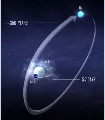
The star δ Ori A (HD 36 486, Mintaka, HIP 25 930, HR 1852) is a massive triple system (see artist’s illustration in Figure 1) comprised of the close eclipsing binary Aa
(primary Aa1, secondary Aa2) with a 5.732-day period (Harvey et al. 1987; Harvin et al. 2002; Mayer et al. 2010),
and the more distant tertiary Ab at an angular separation of 0. 3
» relative to the binary Aa with a period of ∼346 years (Heintz1980; Perryman & ESA1997; Tokovinin et al.2014).
The tertiary Ab has been photometrically resolved from the binary Aa in different surveys (Horch et al. 2001; Mason et al. 2009; Maíz Apellániz2010) and is found to contribute
25%
» to the system’s flux in the visual band. These three components are not to be confused with the more distant and significantly fainter stars δ Ori B and C at separations of 33″ and 53″, respectively; together, these five stars comprise the multiple system δ Ori, also known as Mintaka. With a visual magnitude of V =2 . 24m outside eclipse (Morel & Magne-nat 1978), δ Ori A is one of the brightest massive multiple
systems in the night sky, making it easily visible to the naked eye(it is the westmost star in Orion’s belt). According to the new Hipparcos reduction(van Leeuwen2007), its parallax is
4.71± 0.58 mas, corresponding to a distance of d=212 30 pc.14On the other hand, the system resides in the Orion OB1b association, to which theσ-Orionis cluster belongs as well. The distance to the cluster itself is estimated to be d~380pc, almost a factor of two larger than the Hipparcos distance(see Caballero & Solano2008and references therein).
This paper is a contribution to a series of papers within the framework of theδ Ori collaboration. The other papers include the analysis of high quality Chandra observations to explore X-ray properties(Corcoran et al.2015; Paper I) and variability (Nichols et al.2015; Paper II) in the system, and a complete photometric and spectrometric variabilty analysis(Pablo et al.
2015; Paper III). In this study, we focus on a non-LTE, multiwavelength spectral analysis of the three components Aa1, Aa2, and Ab, with the goal of obtaining reliable stellar and wind parameters.
δ Ori A has been repeatedly studied previously. The system, which shows clear evidence for a significant stellar wind in the optical, UV, and X-ray domains, has been assigned the spectral type O9.5 II(Walborn1972), later refined by Sota et al. (2011)
to O9.5 II Nwk, which most probably corresponds to the brigtest component: Aa1. With less confidence, the secondary Aa2 has been assigned the spectral type B0.5 III (Harvin et al.2002). This result is questioned by Mayer et al. (2010),
who argue that the secondary is too faint for this spectral type. The latter authors further suggest the spectral type O9 IV for the tertiary and leave the secondary unclassified.
Although the stellar parameters of an eclipsing stellar system can usually be sharply constrained, much controversy is found in the literature in the case ofδ Ori A. Koch & Hrivnak (1981)
reported M1=23M, R1=17R and M2=9M,
R2 =10R for the primary and secondary masses and radii,
respectively, as well as a V-band magnitude difference of
VAa1Aa2 1 . 4m
D = . Harvin et al. (2002) later inferred
signifi-cantly smaller masses for the primary and secondary,
M1=11.2M, M2=5.6M, and a smaller contribution of
the secondary in the visual band: DVAa1Aa2=2 . 5m . These results were challenged by Mayer et al.(2010), who suggested
that a confusion between the secondary Aa2 and tertiary Ab led to the low masses obtained by Harvin et al.(2002). Mayer et al.
(2010) inferred R1=15.6R and R2=4.8R. They did not
detect any contribution from the secondary Aa2 and concluded that DVAa1Aa2 3 . 5m . Assuming M1=25M, they inferred
M2=9.9M. In Paper III, the secondary’s radial velocity
(RV) curve could not be constructed, and, for an adopted primary mass of M1»24M, it was concluded that
M2=8.5MR1=15.1R, R2 =5.0R.
Similarly, reported values of the mass-loss rate of the primary are quite diverse: Lamers & Leitherer (1993) report
M
log ˙1= -5.97(Myr )-1 based on radio observation and
M
log ˙1= -5.92(Myr )-1 based on Hα analysis. Lamers et al.
(1999) later similarly obtain log ˙M1= -5.7(Myr )-1 based
on P Cygni profile analysis using the Sobolev plus exact integration method. Neglecting the effects of wind inhomo-geneities and porosity (Oskinova et al. 2007; Šurlan Figure 1. Artist’s impression of the triple system δ Ori A, as viewed from
Earth. The primary(Aa1) and Secondary (Aa2) form the tight eclipsing binary of a period of 5.7 days. The primary shows evidence for a significant wind in all spectral domains. A third star (Ab) at an angular separation of 0. 3» ( 100 AU~ at a distance of d= 380 pc to Earth) orbits the system with a period of≈346 years (Tokovinin et al.2014) and contributes roughly 25% to the total
visualflux. The sizes of all three components are drawn to scale, as inferred in this collaborative study. Their colors reflect their relative temperatures. Note that the tertiary is the second brightest companion in the system. The distance between the binary system Aa and the tertiary Ab is not to scale. Credits to Jessica Mayo.
14
This value is not corrected for the Lutz–Kelker effect (Lutz & Kelker1973).
Maíz Apellániz et al.(2008) account for this effect and revise the distance to
d = 221 pc. However, the difference is negligible within measurement uncertainties.
et al. 2013) on the observed X-ray spectrum, and adopting a
generic O-type model, Cohen et al.(2014) derived a value of
M˙1= -7.2(Myr )-1 from X-ray line profile fitting, more than
an order of magnitude less than the previously inferred value. Indeed, no consensus on the mass-loss rate of the primary has been reached so far.
δ Ori A has an observed X-ray luminosity of
LX»1.4 · 1032erg s-1for d = 380 pc (Paper I). δ Ori A’s X-ray properties were previously explored by Miller et al. (2002), Leutenegger et al. (2006), and Raassen & Pollock
(2013). These studies generally identify the X-ray formation
process to be intrinsic to the primary’s wind, a result that is further supported within our collaboration. An extensive review of past X-ray observations and analyses are given by Paper I
and II.
In this study, we perform a consistent non-LTE photosphere and wind analysis of the three components of the triple system δ Ori A in the optical, UV, and X-ray domains, at several orbital phases. We analyze the optical and UV spectra using the non-LTE Potsdam Wolf–Rayet (PoWR) code, which is applicable to any hot star. We further illustrate the importance of optically thin and optically thick clumps in the wind. We use the non-LTE models to simulate the effect of X-rays in the wind of the primary and derive onset radii of X-ray formation regions using ratios of forbidden and intercombination lines in the Chandra spectra. Finally, using the non-LTE model of the primary, we calculate synthetic X-ray line profiles and compare them to observed ones. Our results are further compared to studies of the radio emission from the system. This study thus encompasses the whole range from the X-ray domain to the radio domain.
The structure of the paper is as follows. In Section 2, we describe the observational data used. Our modeling methods and assumptions are discussed in Section 3. In Section 4, we present and discuss our results. Section5focuses on the effect of wind inhomogeneities on the optical, UV, and X-ray spectral domains, while, in Section 6,we study the X-ray radiation of the star. Lastly, in Section 7, we summarize our results.
2. OBSERVATIONAL DATA
All spectra used in this analysis contain the contribution of the primary Aa1, secondary Aa2, and tertiary Ab. In the following, all phases given are photometric phases relative to primary minimum (occurring when the secondary occults the primary), calculated with E0=HJD 2456277.79d and
P=5.732436 d (Paper IIIand references therein).
Two of our optical spectra are of high resolution and high signal-to-noise ratio (S/N), obtained with the NARVAL spectropolarimeter on 2008 October 23 and 24. These spectra were reduced with standard techniques and downloaded from the PolarBase15 (Petit et al. 2014). The observations were
carried out with the Telescope Bernard Lyot. The spectra have an S/N of 500–800, and correspond to phasesf =0.84 and
0.02
f = .
Three additional optical spectra at phases ϕ = 0.19, 0.38, and 0.54 were obtained on the nights of 2012 December 28, 29, and 30 (contemporaneous with our Chandra and MOST observations) using the CAFÉ spectrograph at the 2.2 m Calar Alto telescope as part of the CAFÉ-BEANS project, a survey that is obtaining high-resolution (R ~ 65,000) multi-epoch
optical spectroscopy of all bright O stars in the northern hemisphere to complement OWN, the equivalent southern hemisphere survey (Barbá et al. 2010; Sota et al. 2014). On
each date, 10 consecutive 30 s exposures were obtained and combined to yield spectra with S/N varying from∼200 in the blue part( 4500~ Å) to ∼500 in the red part ( 6000~ Å). The data were processed using a pipeline developed specifically for the project. The velocity stability was checked using ISM lines. More details regarding the reduction pipeline are given by Negueruela et al.(2014).
For the spectral range 1200–2000 Å, we make use of archival IUE spectra at different orbital phases (see the observation log given by Harvin et al. 2002). The spectra
have an S/N of~10pixel−1, and are averaged in bins of 0.1 Å. The IUE spectra areflux-calibrated and are rectified using the model continuum.
In the spectral range 1000–1200 Å, we make use of the Copernicus observation available in the Copernicus archive under the ID c025-001.u2. This observation consists of 48 co-added scans obtained between 1972 November 21 and 24.
For the spectral energy distribution(SED), we make use of U, B, V, R, I, J, H, K(Morel & Magnenat1978), WISE (Cutri
et al. 2012), and IRAS (Moshir et al. 1990) photometry. We
further use a low-resolution, flux calibrated optical spectrum kindly supplied to us by S. Fabrika & A. Valeev(2015, private communication). The spectrum was obtained with the Russian BTA telescope using the SCORPIO focal reducer, on 2013 December 31 in the range of 3800–7200 Å with a spectral resolution of 6.3 Å, and corresponds to phase f =0.42. A Hartmann mask was used to avoid saturation.
The Chandra X-ray spectra used in Section 6 were taken with the HEG and MEG detectors for a total exposure time of 487.7 ks. The data are thoroughly described inPaper I andII.
3. NON-LTE PHOTOSPHERE AND WIND MODELING 3.1. The PoWR Code
PoWR is a non-LTE model atmosphere code especially suitable for hot stars with expanding atmospheres.16The code consists of two main parts. In the first part, referred to as the non-LTE iteration, the co-moving frame radiative transfer in spherical symmetry and the statistical balance equations are solved in an iterative scheme under the constraint of energy conservation, yielding the occupation numbers in the photo-sphere and wind. The second part, referred to as the formal integration, delivers a synthetic spectrum in the observer’s frame. The pre-specified wind velocity field takes the form of a β-law (Castor et al. 1975) in the supersonic region. In the
subsonic region, the velocity field is defined so that a hydrostatic density stratification is approached. Line blanketing by the iron lines is treated in the superlevel approach(Gräfener et al. 2002), as originally introduced by Anderson (1989). A
closer description of the assumptions and methods used in the code is given by Gräfener et al. (2002) and Hamann &
Gräfener(2004).
In the non-LTE iteration, line profiles are Gaussians with a constant Doppler width vDop. In the formal integration, the
Doppler velocity is composed of depth-dependent thermal motion and microturbulence. The microturbulence x( )r is interpolated between the photospheric microturbulence
15
http://polarbase.irap.omp.eu
16
PoWR models of Wolf–Rayet stars can be downloaded athttp://www.astro. physik.uni-potsdam.de/PoWR.html.
r
(ph) ph
x =x and the wind microturbulence x( )rw =xw, with
the radii rph and rw pre-specified. Thermal and pressure
broadening are accounted for in the formal integration. Turbulence pressure is also accounted for in the non-LTE iteration. Optically thin wind inhomogeneities are accounted for in the non-LTE iteration using the so-called “microclump-ing” approach (Hamann et al. 1995). The density contrast
between a clumped and a smooth wind with an identical mass-loss rate is described by the depth-dependent clumping factor D (r) (Hamann & Koesterke 1998), where the clumps are
assumed to be optically thin. Optically thick clumps, or “macroclumps,” are accounted for in the formal integration as described by Oskinova et al. (2007), where the clump
separation parameter Lmac is to be specified (see Section5).
Four fundamental input parameters define a model atmo-sphere of an OB type star: T*, L, g*, M˙ . T* is the effective
temperature of a star with luminosity L and radius R*, as
defined by the Stefan–Boltzmann relation L=4psR T*2 *4. g*is
related to the radius R* and mass M* via
g g R G M R
* ( *) * *
2
= = - . M˙ is the mass-loss rate of the star.
The stellar radius R* is defined at the continuum Rosseland
optical depth tRoss = 20, which is the inner boundary of our
model, and which was tested to be sufficiently large. The outer boundary of the model is set to100 *. Note that the stellarR
radius is generally not identical to the photospheric radius R2 3
defined attRoss=2 3. However, usually R*@R2 3, except in
cases of extreme radiation pressures (e.g., supergiants, Wolf– Rayet stars). Nevertheless, one must bear in mind that the effective temperature referring to the photospheric radius, which we denote with T2 3 to avoid ambiguity, may slightly
differ from T*. Similarly, g2 3=g R( 2 3) is the gravity at
2 3
Ross
t = . Like most studies, we specify photospheric values when compiling our results in Table1, but the cautious reader should be aware of this difference when comparing with other studies.
Due to the strong radiative pressures in massive stars, one cannot measure the gravity g*directly from their spectra, but
rather the effective gravity geff. g* is obtained from geff via
(
)
g g
* 1
eff ≔ - Grad , where Grad is a weighted average of the
ratio of total outward radiative force to inward gravitational force over the hydrostatic domain. The outward radiative force is calculated consistently in the non-LTE iteration, and includes the contribution from line, continuum, and Thomson opacities (Sander et al.2015).
3.2. The Analysis Method
The analysis of stellar spectra with non-LTE model atmo-sphere codes is an iterative, computationally expensive process that involves a multitude of parameters. Nevertheless, most parameters affect the spectrum uniquely. Generally, the gravity g*is inferred from the wings of prominent hydrogen lines. The
stellar temperature T* is obtained from the line ratios of ions
belonging to the same element. Wind parameters such as M˙ ,
v¥, and Lmacare derived from emission lines, mainly in the UV.
The luminosity L and the color excess E B( -V) are determined from the observed SED, and from flux-calibrated spectra. The abundances are determined from the overall strengths of lines belonging to the respective elements. Finally, parameters describing the various velocity fields in the photosphere and wind (rotation, turbulence) are constrained
from profile shapes and strengths. The radius R*and
spectro-scopic mass M*follow from L, T*, and g*.
To analyze a multiple system such asδ Ori A, a model for each component star is required. As opposed to single stars, the luminosities of the components influence their contribution to the overall flux and thus affect the normalized spectrum. The light ratios of the different components therefore become entangled with the fundamental stellar parameters. Fortunately, with fixed temperatures and gravities for the secondary and tertiary components, the observational constraints provide us with the light ratios(see Section3.3).
Methods to disentangle a composite spectrum into its constituent spectral components by observing the system at different phases have been proposed and implemented during the past few years (Bagnuolo & Gies 1991; Simon & Sturm1994; Hadrava 1995; González & Levato2006; Torres et al.2011). In fact, an attempt to disentangle the spectrum of
δ Ori A was pursued by Harvin et al. (2002) and Mayer et al.
(2010). However, even after performing the disentanglement,
the two sets of authors come to significantly different results. A disentanglement of the HeIl6878line was performed inPaper III, but, after accounting for the contribution of the tertiary as obtained here, no clear signal from the secondary was detected. Given the very low contribution of the secondary Aa2, and having only poor phase coverage in the optical, we do not pursue a disentanglement ofδ Ori A.
As a first step, the secondary and tertiary models are kept fixed. Motivated by the results ofPaper III, we initially adopt
T2 3~25kK and logg2 3~4.15(g cm )-2 for the secondary.
The tertiary is initiallyfixed with the parameters suggested by Mayer et al.(2010). With the light ratios at hand, this fixes the
luminosities of Aa2 and Ab. Havingfixed the secondary and tertiary models, we turn to the second step, which is an accurate analysis of the primary.
To constrain T*, we use mostly HeI and HeIIlines, such as
HeIll 4026, 4144, 4388, 4713, 4922, 5015, 6678 and HeII
λ4200, 4542, 5412, 6683. The prominent HeIIl4686 line is
found to be a poor temperature indicator(see Section4.2). The
temperature is further verified from lines of carbon, nitrogen, and silicon. g* is primarily derived from the wings of
prominent Balmer and HeII lines. Here we encounter the
difficult problem of identifying the contribution of the tertiary to the hydrogen lines due to the pronounced wings of the Balmer lines. We therefore also made use of diagnostic lines such as CIIIl5696, whose behavior heavily depends on the
gravity(see Section4.4).
M˙ and Lmac follow from a simultaneous fitting of Hα and
UV P Cygni lines. The wind parameters are checked for consistency with previous analyses of radio observations and with X-ray observations (see Section 6.3). The terminal
velocity v¥ is determined from UV resonance lines. However,
v¥ can only be determined accurately after the wind microturbulence has been deduced. The determination of the projected rotational velocity vsini and of the inner (photo-spheric) and outer (wind) microturbulent velocitiesx andph x ,w as well as of the macroturbulent velocity vmac, is discussed in
detail in Section4.3.
The abundances are determined from the overall strengths of lines belonging to the respective elements. We include the elements H, He, C, N, O, Mg, Al, Si, P, and S, as well as elements belonging to the iron group (e.g., Fe, Ni, Cr etc.).
With the remaining stellar parameters fixed, this is a straightforward procedure.
The total bolometric luminosity L=L1+L2+L3 is
obtained by fitting the synthetic flux with the observed SED. The individual component luminosities follow from the light ratios. The color excess EB-V is derived using extinction
laws published by Cardelli et al.(1989) with RV= 3.1, and can
be very accurately determined from flux-calibrated IUE observations. The inferred value for AV is consistent with
those of Maíz Apellániz & Sota (2015, in preparation), who obtain a value of 0.185 ± 0.013 mag using Tycho+Johnson +2MASS photometry and the extinction laws of Maíz Apellániz et al. (2014).
After obtaining a satisfactory model for the primary, we continue to iterate on the secondary and tertiary models by identifying small deviations between the composite synthetic and observed spectra at different orbital phases, as described in Section 4.2. This allows us to adjust the temperatures and gravities of both models, as well as of the projected rotation velocities. After improving the secondary and tertiary models, we return to the primary and adjust the model parameters accordingly. We repeat this process several times until a satisfactory fit is obtained in the UV and optical, taking hundreds of lines into account in this process.
3.3. Initial Assumptions
Given the large number of parameters involved in this analysis, it is advisable to initially fix parameters that are constrained based on observations, previous studies, and theoretical predictions.
We adopt β = 0.8 for the exponent of the β-law for all components, which is both supported by observations as well as theoretically predicted (e.g., Kudritzki et al. 1989; Puls et al.1996). Varying this parameter in the range 0.7–1.5 did
not significantly affect the resulting synthetic spectrum. A V-band magnitude difference ofDVAaAb=1 . 35m between the binary system Aa (composed of Aa1 and Aa2) and the tertiary Ab was measured by the Hipparcos satellite(Perryman & ESA 1997). Horch et al. (2001) report VD AaAb=1 . 59m , obtained from speckle photometry. Mason et al. (2009) find
VAaAb 1 . 4m
D = by means of speckle interferometry. Like Mayer et al.(2010), we adopt VD AaAb=1 . 4m , corresponding to the flux ratio RAaAb≔FV(Aa) FV(Ab)=3.63. As for the binary components Aa1 and Aa2, additional information regardingDVAa1Aa2can be obtained from the visual light curve
of the system δ Ori A. The secondary light curve minimum (primary star in front) has a depth VD II. min»0 . 055m with an error of about 0 . 005m . Since the secondary eclipse is partial (Paper III), the secondary minimum yields a lower limit to
Table 1
Inferred Stellar Parameters for the Multiple Stellar Systemδ Ori A
Aa1 Aa2 Ab T2 3(kK) 29.5± 0.5 25.6± 3000 28.4± 1500 g log eff(cm s-2) 3.0± 0.15 3.7 3.2± 0.3 g log 2 3(cm s−2) 3.37± 0.15 3.9 3.5± 0.3 v¥(km s−1) 2000± 100 1200 2000 D 10 10 10 Lmac(R) 0.5 L L E B( -V)(mag) 0.065± 0.01 0.065± 0.01 0.065± 0.01 AV(mag) 0.201± 0.03 0.201± 0.03 0.201± 0.03 vsini(km s−1) 130± 10 150± 50 220± 20 ph x (km s−1) 20± 5 10 10± 5 w x (km s−1) 200± 100 10 10 vmac(km s−1) 60± 30 0 50± 30 H(mass fraction) 0.70± 0.05 0.7 0.7 He(mass fraction) 0.29± 0.05 0.29 0.29 C(mass fraction) 2.4 1´10-3 2.4´10-3 2.4´10-3 N(mass fraction) 4.0 2´10-4 7.0´10-4 7.0´10-4 O(mass fraction) 6.0 2´10-3 6.0´10-3 6.0´10-3 Mg(mass fraction) 6.4´10-4 6.4´10-4 6.4´10-4 Al(mass fraction) 5.6´10-5 5.6´10-5 5.6´10-5 Si(mass fraction) 4± 2 × 10⁻⁴ 6.6´10-4 6.6´10-4 P(mass fraction) 5.8´10-6 5.8´10-6 5.8´10-6 S(mass fraction) 3.0´10-4 3.0´10-4 3.0´10-4 Fe(mass fraction) 1.3´10-3 1.3´10-3 1.3´10-3 Adopted distance d(pc) 212 380 212 380 212 380 L log (L) 4.77± 0.05 5.28± 0.05 3.7± 0.2 4.2± 0.2 4.3± 0.15 4.8± 0.15 M log ˙ (M yr -1) −6.8 ± 0.15 −6.4 ± 0.15 −8.5 −8.1 ⩽-7.0 ⩽-6.6 Mspec(M) 7.5-+2.53 24+-108 2.6 8.4 7.0-+47 22.5-+1424 R2 3(R) 9.2± 0.5 16.5± 1 3.6± 1 6.5-+1.52 5.8± 1 10.4± 2 MV(mag) −4.47 ± 0.13 −5.74 ± 0.13 −1.7 ± 0.5 −3.0 ± 0.5 −3.2 ± 0.4 −4.5 ± 0.4
RAa2Aa1. One obtains after some algebra
(
)(
)
R R R R R 1 1 1 . (1) Aa2Aa1 II.min AaAb AaAb II.min - + - + ⩾In our case, RAaAb»3.63 and RII.min »1.05, and so
FV(Aa2) 0.07FV(Aa1), which in turn implies DVAa1Aa2
2 . 9m . It follows that the secondary Aa2 contributes at least
6.5% to the visualflux of the binary, and at least 5.1% to the total visual flux of the system. We thus initially assume
VAa2Aa1 2 . 8m
D = , and further constrain this value in the spectral analysis (see Section4.1).
In Section4.1, we show that usage of the Hipparcos distance
d =212 pc results in extremely peculiar parameters for the primary given its spectral type, and that a much better agreement is obtained for the alternative distance of the neighboring stellar cluster σ-Orionis, d~380pc(see also the discussion by Simón-Díaz et al. 2015). We therefore refer to
both distances in the following and discuss this issue more thoroughly in Section 4.1. We note, however, that our results can be easily scaled with the distance, should it be revised in future studies (see Section4).
As we illustrate in Section5, there are several indications for wind inhomogeneities (clumps) in the wind of Aa1. While clumping may already initiate at sub-photospheric layers, e.g., due to sub-photospheric convection (Cantiello et al. 2009),
we avoid an attempt to treat clumpiness in the optically thick layers below the photosphere. For reasons that are discussed in detail in Section 5, we adopt a depth-dependent clumping factor D(r) that is fixed to one (no clumping) in the domain
R r R
*⩽ ⩽1.1 *and reaches a maximum value of Dmax=10
at r⩾10 *R .
Due to the faintness of the secondary and tertiary, we can only give upper limits to their mass-loss rates, and set their terminal velocities to be 2.6 times their escape velocity (Lamers & Cassinelli 1999). We further assumex( )r =10km s−1for the secondary, a typical value for OB-type stars of luminosity classes III and lower (see Villamariz & Herrero 2000 and references therein). We choose to adopt an identical density contrast D(r) for all three models. Finally, we do not attempt to constrain the abundances in the secondary and tertiary, but rather adopt solar values(Asplund et al.2009). This set of assumptions
should bear very little effect on the derived fundamental parameters of the three components.
4. RESULTS
The stellar parameters inferred for the three components are given in Table1. The model of the primary includes the effect of macroclumping and X-rays, which we thoroughly discuss in Sections 5 and 6. The upper part of the table displays parameters that, to first order, do not depend on the adopted distance. The lower part of the table denotes distance-dependent parameters. For the convenience of the reader, we give these parameters for both “candidate” distances,
d =212 pc and d=380pc. Luminosities scale as Lµd2,
mass-loss rates as M˙ µd3 2, radii as R d
* µ , and the mass as
Mspecµd2. The error margins given in Table1are discussed in
Section 4.4and are based on the sensitivity of our analysis to these parameters. Values without errors that are not upper bounds indicate adopted values.
The upper panel of Figure2displays the synthetic SEDs for the models of the three components of the system. The total
synthetic SED(red solid line) comprises the synthetic fluxes of the primary Aa1(green dashed line), secondary Aa2 (gray dot– dashed line), and tertiary Ab (pink dotted line). Recall that the tertiary is brighter than the secondary. The blue squares denote U, B, V, R, I, J, H, K, WISE, and IRAS photometry. We also plot two observedflux-calibrated spectra in the UV and optical (blue lines). The lower panels of Figure2show the composite synthetic(red dotted line) and observed (blue line) normalized UV and optical spectra of the system. The optical spectrum and the UV spectrum in the range 1200–2000 Å correspond to phasef »0.54. The synthetic normalized spectrum consists of three models calculated for Aa1, Aa2, and Ab, shifted according to their RVs. The synthetic spectra are convolved with a Gaussian of FWHM= 0.1 Å to account for instrumental broadening, inferred from fitting of the interstellar NaI
5890, 5896.3
ll lines. We do not plot the individual spectra of the three components for clarity. Note that the wavy pattern seen in the observed spectrum (e.g., in the domain 5900–6500 Å) is an artifact that originates in the connection of the echelle orders, not related to the stellar system.
It is evident that both the synthetic SED and normalized spectrum agree well with the observed spectrum. A good balance is obtained for all HeIlines and HeIIlines, as well as
for the metal lines. The inferred parameters for microturbu-lence, rotation, and macroturbulence yield consistent line strengths and profiles over the whole spectral domain. The pseudo continuum formed by the iron forest in the range of 1300–1800 Å, as well as most photospheric and wind features, are well reproduced.
The few features that are not reproduced very well are the Balmer lines, and especially Hδ. Hδ has a significantly smaller observed EW ( 1.85» Å) compared to the synthetic spectrum ( 2.35» Å). In fact, the observed EW of Hδ is somewhat smaller than usual for similar spectral types(e.g., Cananzi et al.1993),
and the question arises as to the cause. A significantly smaller gravity for the primary does not agree with the wing shape of the other Balmer and HeII lines and hardly affects the EW.
Reducing the hydrogen abundance of the primary implies a larger helium abundance, which is not consistent with the helium lines. Larger M˙ values lead to very strong emission in Hα, which is not observed. The photospheric microturbulence has only negligible effect on the EW of hydrogen lines. We therefore conclude that the Balmer lines are dilluted by the light of one or both of the other components. However, the low EW of Hδ could only be reproduced when assuming very peculiar parameters for the tertiary, e.g., a very weak gravity(logg2 33.2(g cm )-2), or very large mass-loss rates (log ˙M -5.5
(
M yr-1)
). Such parameters are not only hard
to justify physically, but also not consistent with the remaining spectral lines. The problem is also seen, albeit to a lesser extent, in the lines Hγ and Hβ. Future observations should shed light on this peculiarity.
4.1. Which Distance is the Correct one?
It is reassuring that those fundamental stellar parameters of the primary that do not depend on the distance match well with its spectral type. Interpolating calibrations by Martins et al. (2005) to an O9.5 II class yields T2 3=29.3kK and
g
log 2 3=3.35(g cm )-2, which agrees with our results within the error margins. The primary’s nitrogen and silicon abundances are found to be slightly subsolar. It is interesting
to note that Sota et al.(2011) recently added the suffix “Nwk”
to the spectral type of Aa1, implying relatively weak nitrogen lines, which we confirm independently.
For d = 380 pc, the distance-dependent parameters agree well with calibrations by Martins et al. (2005). Interpolating
to luminosity class II, calibrations by Martins et al. (2005)
imply logL L=5.3, M=25M, R2 3=18.2R, and
MV = -5 . 73m for an O9.5 II star, which is consistent with our results. Furthermore, this distance implies radii and masses for the primary and secondary that agree well with the results obtained independently in Paper III. However, very peculiar values are obtained when using the Hipparcos distance of
d =212 pc (see lower part of Table 1). In fact, all three
components appear to be peculiar when adopting the Hipparcos distance. While a membership in a close binary system offers some room for deviations from standard values, this would not explain why the distant tertiary Ab should be peculiar too. The fact that distance-independent parameters are not unusual raises even more suspicion regarding the Hipparcos distance.
A similar discrepancy is observed in other bright stars: Hummel et al.(2013) analyzed the binary system ζ Orionis A
(V = 1.79) and inferred a distance of d=29421 pcbased on an orbital analysis, and d=38754 pc based on a photometric estimate. Both of these distances are significantly larger than the corresponding Hipparcos distance of Figure 2. Upper panel: comparison between observations (blue squares and lines) and the total synthetic SED (red solid line), which consists of the primary (green dashed line), secondary (gray dash–dotted line), and tertiary (pink dotted line) models. Lower panels: comparison between the composite synthetic (red dotted line) and observed(blue line) normalized spectra in the UV and optical. Both spectra roughly correspond to phasef =0.54. For clarity, we refrain from showing the contributions of each component model to the normalized spectrum. The wavy pattern seen in the observed spectrum(e.g., in 6000 6200» - Å) is an artifact caused by connecting the echelle orders, not related to the stellar system.
d =225-+2738pc (van Leeuwen2007), which encouraged them to discard the Hipparcos distance in their study. Another bright star for which the Hipparcos parallax implies very peculiar stellar parameters is the prototypical O supergiant ζ Puppis (V = 2.25). Its distance was suggested to be at least twice as large as implied by its measured parallax (Pauldrach et al.
2012; Howarth & Stevens 2014).
Returning to δ Ori A, our estimate of d~380 pc would correspond to a parallax ofp ~2.6mas, deviating by~3.5s from the newly reduced Hipparcos parallax of 4.71± 0.58 mas (van Leeuwen 2007). The probability for such a deviation to
arise randomly is thus extremely small( 0.1%< ). Ground-based parallaxes for δ Ori A generally suffer from much larger uncertainties. For example, the Yale catalog gives
9.7 6.7
p = mas (van Altena et al. 1995). It is interesting
to note that the original Hipparcos catalog gives a parallax of 3.560.83 mas (ESA 1997a, 1997b). In this case, the
deviation could be plausibly explained as a random error, with 2.6 mas being~1s away. While stellar multiplicity has been suggested to cause systematic errors in parallax measurements (e.g., Szabados 1997), the argument is unlikely to hold here
given the different timescale of the involved orbits compared to that of the parallax measurement (which is to say, a year). However, large errors in the parallax measurement are also expected to occur in the case of very bright stars, which could lead to saturation, resulting in an inaccurate estimate of the barycenter of the point-spread function. Brightness is indeed a propertyδ Ori A shares with the objects mentioned above. It is beyond the scope of the paper to judge whether the new Hipparcos reduction suffers from underestimated errors, but the fact that several bright stars show a similar pattern should encourage thorough studies on the matter.
The distance to δ Orionis is difficult to directly measure with modern techniques. The system is probably too bright for ground-based(e.g., RECONS)17as well as space-based instruments(e.g., the Hubble Space Telescopeʼs Fine Guidance Sensor; the Gaia mission). Our best hope is to obtain the RV curve of the secondary, which requires optical spectroscopy with an S/N
1000
(Paper III). Then, with a direct measure of the system
parameters, follow-up long-baseline interferometry may provide the angular extent of the orbit, allowing for an orbital parallax measurement similar to that ofζ Ori A (Hummel et al.2013). At
380 pc, the angular extent of the orbit will be on the order of 0.5 mas and thus difficult to measure, as the smallest angular separation for a binary yet resolved is 1.225 mas (Raghavan et al. 2009). However, this was done in the K-band with the
CHARA Array, so the resolution in the R band should be sufficient to resolve the binary. Moreover, along with a light-curve analysis, and possessing both RV light-curves, one could accurately derive the masses and radii of both components, which, upon comparison with a distance-dependent spectral analysis, would supply another constraint on the distance. For now, we suggest that the Hipparcos distance may be underestimated, but leave the question open for future studies to resolve.
4.2. Constraining the Parameters of Aa2 and Ab Thefive columns of Figure3depict six prominent HeIIand
HeI lines, from left to right: HeIIl4686, HeIl4922,
HeII l5411, HeIl5876, and the two adjacent lines HeI
6678
l and HeIIl6683. Each row depicts a different orbital
phase, from top to bottom: f =0.02, 0.19, 0.38, 0.54, 0.84. This time, we explicitly show the relative contributions of the primary(green dashed line), secondary (gray solid line), and tertiary (pink dot–dashed line) to the total synthetic spectrum (red dotted line), compared to the observations at each phase (blue line). In Table2, we specify the RVs with which the three components are shifted at each phase. The RVs for the primary were inferred in this study and agree very well with the RV curve of Mayer et al.(2010) and those ofPaper III.
4.2.1. The Tertiary
There is a wide and shallow spectral feature that does not originate in the primary and is constant along all orbital phases (see Figures3 and 4). Like Mayer et al. (2010), we identify
this feature with the tertiary Ab, which is in fact the second brightest source in the system. The RV of the tertiary, which is practically constant over all phases, is also inferred indepen-dently, and agrees well with that suggested by Mayer et al.(2010).
Wefind that the tertiary contributes significantly more to HI
lines than to HeII lines. Together with the visual flux ratio
implied from observations, this leads to a tertiary temperature of T*~29.0kK. The gravity and mass-loss of the tertiary were constrained based on the Balmer lines. As already discussed, it is very hard to identify the explicit contribution of the tertiary to these lines, and so the gravity and mass-loss of the tertiary are only roughly constrained. The parameters derived for the tertiary(see Table1) are consistent with it being a B0 IV-type
star(Habets & Heintze1981; Schmidt-Kaler1982).
4.2.2. The Secondary
It is very hard, or perhaps impossible, to recognize any contribution from Aa2 to the spectrum. One exception might be the HeIlinesll4026, 4144at phasef =0.84, which we show
in the left and right panels of Figure4, respectively(colors and lines are as in Figure 3). At this phase, the primary’s RV
approaches its maximum of∼110 km s−1, and so the secondary is expected to be more easily observed. The HeIl4026 line, for
example, seems to have an extended wing toward blueshifted wavelengths. The very weak HeIl4144 line is one of the few
spectral lines that possibly portrays a partially isolated feature originating in the secondary. We therefore infer an RV for the secondary in this phase. For all other phases, we adopt the secondary’s RVs from Harvin et al. (2002), since the secondary’s
lines cannot be isolated in the spectrum. However, as Mayer et al. (2010) pointed out, it is likely that Harvin et al. (2002) confused
the secondary with the tertiary, so that the secondary RVs reported by Harvin et al.(2002) are questionable.
Even without directly detecting the secondary, we can still constrain its stellar parameters. Since the light curve provides a lower limit for its visualflux (see Section3.3), the luminosity of
Aa2 cannot be arbitrarily small. Instead, to avoid too-strong line features from the secondary(which are not observed), we are forced to change other stellar parameters, e.g., T*and vsin .i
The secondary’s projected rotation velocity (vsini»150 km s−1) agrees with the feature shown in the right panel of Figure 4, and the secondary temperature (T»26kK) is consistent with that obtained from the light curve analysis of the system(Paper III).
In Section 3.3, we argued that the light curve of δ Ori Aa implies that the secondary contributes at least 5.4% to total
17
visual flux of the system. In this section, we argue that the secondary can contribute no more than this amount. In other words, our lower bound for the relative flux contribution becomes also our upper bound, and thereforeDVAa1Aa2»2 . 8m . Together with the temperature of the secondary, this enables us to infer an approximate value for the luminosity of the secondary. Its parameters suggest it is a ≈ B1 V type star (Habets & Heintze1981; Schmidt-Kaler1982).
4.3. Bulk and Turbulent Motions
4.3.1. Rotation and Macroturbulence
Rotation is usually the dominant broadening mechanism of photospheric metal lines in OB type spectra, as is the case here. Figure 3. Twenty-five panels show the contribution of the primary (green dashed line), secondary (gray solid line), and tertiary (pink dash–dotted line) models to the composite synthetic spectrum(red dotted line) for six prominent helium lines and five different phases, compared with observations (blue line). The lines depicted are, from left to right, HeIIl4686, HeIl4922, HeIIl5411, HeIl5876, and the two adjacent lines HeIl6678and HeIIl6683. The phases are, from top to bottom,
0.02, 0.19, 0.38, 0.54
f = , and 0.84. At each phase, the component models are shifted with the velocities given in Table2.
Table 2
Radial Velocities Derived/adopted for each Phase in km s−1
Phase Aa1a Aa2b Aba
0.02 0 10 25 0.19 −92 230 25 0.38 −22 120 25 0.54 83 −100 25 0.84 105 −210 25 Notes. a
Values for primary and tertiary derived in the analysis.
b
Values for secondary adopted from Harvin et al.(2002), with the exception
We infer the projected rotational velocity vsin by convolvingi
the synthetic spectrum with a rotation profile and comparing the line shapes to the observed spectrum. While flux convolution is a fair approximation for photospheric spectra, it does not account for the effect of limb darkening and for the extended formation regions of some lines. Accounting for rotation in the formal integration is essential for a consistent inclusion of these effects, but is computationally expensive. We therefore use the convolution method to infer vsin , and, onlyi
after obtaining the best-fit value of vsin , do we account fori
rotation directly in the formal integration (see Hillier et al. 2012; Shenar et al. 2014), assuming co-rotation up of
the photosphere (tRoss=2 3) and angular momentum con-servation in the wind. Compared to simple flux convolution, the detailed treatment of rotation generally yields deeper lines with less elliptic profiles (e.g., Unsöld 1955) and may
significantly affect the inferred abundances, projected rotation velocities, and even fundamental stellar parameters.
The effect of rotation on the spectrum is coupled to the effects of macroturbulence vmac, which we model using a
Radial–Tangential profile (Gray 1975; Simón-Díaz & Her-rero 2007). Macroturbulence does not enter the radiative
transfer per definition. Therefore, like solid body rotation, macroturbulence conserves the EWs of the lines. Typical values of vmac~50km s−1are reported for OB-type stars (Lefever et al. 2007; Markova & Puls 2008; Bouret et al. 2012). While the origin of macroturbulence is not
certain, it has been suggested to be a manifestation of collective pulsational broadening(e.g., Aerts et al.2009). vsin and vi mac
are inferred simultaneously from the profile shapes of helium lines and metal lines. Not accounting for macroturbulence generally results in qualitatively different profiles from what are observed in photospheric lines(see, e.g., example given by Puls et al. 2008).
Harvin et al. (2002) inferred vsini=157km s−1for the primary. While this value agrees well with the wings of prominent helium and metal lines, it leads to too-broad Doppler cores. A significantly better fit is obtained with vmac=60km s−1and
vsini=130km s−1. For an inclination of i=76 (Paper III)
and a radius of R=16.5R(Table1), this could imply that the
rotation period is approximately synchronized with the orbital period of 5.7 days.
For the tertiary, we find an optimal fit for
vsini=220km s−1and vmac=50km s−1, thus confirming the findings of Harvin et al. (2002) and Mayer et al. (2010)
that the tertiary is a rapid rotator. For the secondary, motivated by the arguments discussed in Section 4.2, we estimate
vsini~150km s−1. We adopt vmac=0 for the secondary, lacking any spectral lines from which it can be inferred. Any other typical values would bear no effect on our results.
4.3.2. Microtubulence and Terminal Velocity
In contrast to macroturbulence, microscopic turbulent motion enters directly into the process of radiative transfer and generally affects the EWs of spectral lines. In the non-LTE iteration, we do not specify the microturbulence explicitly, but rather the total Doppler width vDop of the opacity and
emissivity profiles. vDop thus determines the resolution of the
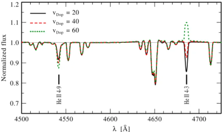
frequency grid in the non-LTE iteration. This parameter generally has a negligible effect on the obtained population numbers, with the extreme exception of the HeIIl4686 line.
As was already noted by Evans et al. (2004), this line reacts
very strongly to changes in vDop. We illustrate this in Figure5,
where we show a segment of the optical spectrum containing the HeII l4686 line. In the figure, we depict three models
corresponding to the primary calculated with parameters identical to those given in Table 1, but with vDop=20, 40, and 60 km s−1, respectively. It is evident that the HeII
4686 Å line reacts remarkably strongly to vDop. The exact
origins of this effect are still under investigation(Shenar et al. 2015, in preparation), but likely involve a feedback effect in the highly nonlinear iterative solution of the radiative transfer problem. The remaining HeII lines show a much weaker
reaction in the opposite direction. Other lines hardly respond to changes of this parameter. This example shows that, overall, the choice of the parameter vDop is not critical for thefit, and
that HeIIl4686is a poor temperature indicator. Based on this,
vDop=30km s−1 is used in the analysis, consistent with the inferred microturbulence(see below).
In the formal integration, apart from including natural and pressure broadening, the Doppler width is separated into a thermal component vth, which follows the temperature
stratification in the model, and a depth-dependent microturbu-lence componentx( )r , which is assumed to be identical for all ions. As described in Section3.1,x( )r is interpolated between Figure 4. Two panels depict two observed HeIlines (blue lines) at phase
0.84
f = in which the secondary may be detectable. The different curves correspond to the primary (green dashed line), secondary (gray solid line), tertiary(pink dash–dotted line), and total (red dotted line) synthetic spectra.
Figure 5. Illustration of the extreme sensitivity of the HeIIl4686line to the parameter vDop. Here we depict only the primary model, calculated with the
parameters in Table 1, but with vDop=20km s−1(black solid line), 40 km s−1(red dashed line), and 60 km s−1(green dotted line). The formal integration is performed with the same turbulent velocity as given in Table1. Notice that most lines hardly react to this parameter.
the photosphericx and windph x turbulent velocities betweenw two pre-specified radii, all of which are free parameters.
Values of photospheric microturbulence reported for O giants range between ∼10 km s−1and 30 km s−1(e.g., Gies & Lambert1992; Smartt et al.1997; Bouret et al.2012). Since the
photospheric microturbulence xph is rarely found to be larger than 30 km s−1, its effect on the profile width is negligible compared to the effect of rotation. However, xph can have a very strong effect on the EW of spectral lines. The abundances are thus coupled tox , and wrong turbulence values can easilyph lead to a wrong estimation of the abundances (e.g., McErlean et al. 1998; Villamariz & Herrero 2000). To disentangle the
abundances and turbulence from, e.g., the temperature, we take advantage of the fact that different lines respond individually to changes in abundances, turbulence, and temperature, depend-ing on their formation process. Figure6shows an example. The left, middle, and right panels depict the HeI l5876 line as
observed at phasef = 0.84(blue line). In each panel, we show three different composite synthetic spectra(i.e., composing all three components), which were calculated with parameters identical to those given in Table 1, except for one stellar parameter of the primary. In the left panel, T*is set to 29.5, 30,
and 30.5 kK. In the middle panel, the helium mass fraction is set to XHeof 0.2, 0.3, and 0.4. Lastly, in the right-most panel,
we set xph to 15, 20, and 25 km s−1, respectively. The three composite spectra at the left and middle panels can hardly be distinguished from each other, portraying the insensitivity of the HeIl5876 line to temperature and helium abundance. In
the relevant parameter domain, it is mainly xph which influences the strength of the HeIl5878line. By considering
hundreds of lines at all available orbital phases, we find that 20
ph
x = km s−1provides the best results for the primary’s model. Similarly, we find that a microturbulence of 10 km s−1for the tertiary yields the best globalfit.
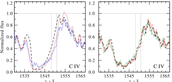
We find evidence for a rapid increase of the turbulent velocity in the primary right beyond the sonic point. The left panel of Figure 7 shows the CIVll1548, 1551 resonance
doublet, as observed in the IUE spectrum taken at phase 0.73
f = . The observation shows a wide absorption trough which extends to redshifted wavelengths, and our task is to reproduce this feature. The black dashed line depicts the composite synthetic spectrum calculated with the parameters in Table 1, but without an increased wind turbulence in the primary model, i.e., xw=xph =20km s−1. The absorption
trough is not reproduced. Increasing the terminal velocity only affects the blue edge of the line. Varying β in the domain 0.7–1.5 does not lead to any notable changes in the spectrum. The only mechanism that is found to reproduce the redshifted absorption trough is a rapid increase of the microturbulence beyond the sonic point. The red solid line was calculated like the dashed black line, but with a wind turbulent velocity of
200
w
x = km s−1. x( )r is assumed to grow from xph at
rin⩽1.1 *R tox at rw out ⩾2 *R . At the same time, the blue
absorption edge is shifted by~200km s−1, thus influencing the value deduced for v¥. The right panel of Figure 7 shows the
same CIVresonance doublet, as observed in three IUE spectra
taken at phases f =0.18, 0.72, 0.98 (black, red, and green lines, respectively). The figure illustrates the relatively small variability of this line, showing that our results do not depend on phase, and rejecting the contamination by another component as an explanation for the extended redshifted absorption. The absorption trough is not reproduced for rout
significantly larger than R2 *, which is understandable given the need for redshifted absorption. It is interesting to note that it is microturbulence, and not macroturbulence, that is needed to reproduce this feature. A further improvement of the line profile fit is obtained by accounting for optically thick clumps (macroclumps) in the wind, as we will discuss in Section5. We do not include macroclumping at this stage in order to single out the effect ofx on the line prow file.
Having inferred the turbulent velocity and after accounting for clumping in the wind of the primary, it is straight-forward to derive the terminal velocity v¥ from resonance P Cygni lines. All prominent lines in the UV imply the same value for
v¥ (2000 ± 100 km s−1).
4.4. Uncertainties
Since the calculation of a PoWR model atmosphere is computationally expensive, a statistical approach for error determination is virtually impossible. The errors given in Table 1 for each physical quantity are obtained by fixing all parameters but one and varying this parameter, estimating upper and lower limits that significantly change the quality of the fit in many prominent lines relative to the available S/N. Errors for parameters that are implied from fundamental Figure 6. Sensitivity of the HeIl5876line to temperature, helium abundance,
and microturbulence. The observed spectrum(blue line) at phasef =0.84is plotted along with three composite synthetic spectra calculated with the parameters given in Table 1, but with different temperature (left panel: T = 29.5, 30, 30.5 kK), helium abundance (middle panel: XHe=0.2, 0.3, 0.4), and photospheric microturbulence (right panel:
15, 20, 25
ph
x = km s−1) for the primary model (black dot–dashed, red dashed, and green dotted lines, respectively).
Figure 7. Left panel: observed CIVresonance doublet at phasef =0.73(blue line) is compared to two synthetic composite spectra, with increased wind turbulence of x =w 200km s−1in the primary model (red solid line), and without it(black dashed line). Large microturbulent velocities beyond the sonic point are the only mechanism that can reproduce the redshifted absorption trough. Note that a further improvement of the profile is achieved by accounting for macroclumps, which are not included here. Right panel: comparison of three IUE observations at phasesf =0.18, 0.73, 0.98(black, red, and green lines, respectively), illustrating that the redshifted absorption trough is observed at all phases.
parameters via analytical relations, e.g., the spectroscopic mass, are calculated by means of error propagation. In the case of multiple systems, all models but one test model are keptfixed, and only one parameter of the test model is varied.
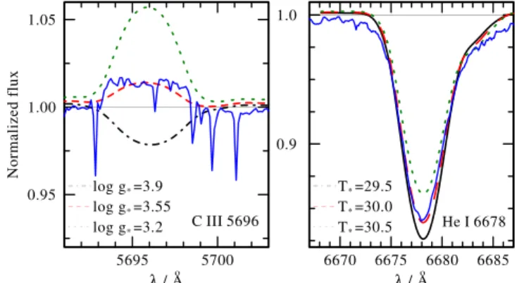
As mentioned in Section 4, it is very hard to constrain the gravity of the primary due to contamination by the other components. However, we took advantage of the fact that specific lines do drastically change their strength as a function of gravity. An example of such a diagnostic line, CIIIl5696, is
shown in the left panel of Figure 8, as observed at phase 0.02
f = (blue line). Three composite spectra (i.e., including all components) are plotted, where only the logg
* of the primary is changed to 3.9 (black dot–dashed line), 3.55 (red dashed line), and 3.2 (g cm )-2 (green dotted line). The remaining stellar parameters are keptfixed to the values given in Table 1. This line only starts to portray emission when
g
log
*~3.5(g cm )
2
- . This line also serves as a good example
of why c2 fitting would not always suggest the best fitting
model. The contribution of such a small line to the reducedc2
is negligible, unlike its diagnostic power. The right panel of Figure 8 depicts the sensitivity of the HeI line to the stellar
temperature. The temperature of the primary is changed to 29.5 (black dot–dashed line), 30 (red dashed line), and 30.5 kK (green dotted line). Most HeIand HeIIlines react strongly to
changes in the temperature and thus enable us to sharply constrain it.
5. INHOMOGENEITIES IN THE PRIMARY’S WIND Evidence for wind inhomogeneities(clumping) in the winds of hot stars are frequently reported. Hillier(1984) and Hillier
(1991) illustrated the effect of optically thin clumps on the
electron scattering wings of Wolf–Rayet emission lines. More compelling direct evidence for clumping in the form of stochastic variability on short timescales was observed in both Wolf–Rayet (e.g., Lépine & Moffat 1999) and OB stars
(Eversberg et al. 1998; Markova et al. 2005; Prinja & Massa
2010). Clump sizes likely follow a continuous distribution
(e.g., power law), which is intimately connected with the turbulence prevailing in the wind (e.g., Moffat 1994).
How-ever, since consistent non-LTE modeling of inhomogeneous
stellar winds in 3D is still beyond reach, the treatment of clumping is limited to approximate approaches.
5.1. Microclumping
A systematic treatment of optically thin clumps was introduced by Hillier(1984) and later by Hamann & Koesterke
(1998) using the so-called microclumping approach, where the
population numbers are calculated in clumps that are a factor of D denser than the equivalent smooth wind. In this approach, processes sensitive to ρ, such as resonance and electron scattering, are not sensitive to clumping, and imply M˙ directly. However, processes that are sensitive to r , such as2
recombination and free–free emission, are affected by clump-ing, and in fact only imply the value of M D˙ . This enables consistent mass-loss estimations from both types of processes, and offers a method to quantify the degree of inhomogeneity in the wind in the optically thin limit.
To investigate wind inhomogeneities in the primary Aa1, we first adopt a smooth model. The four panels of Figure9depict four“wind” lines: three UV resonance doublets belonging to SiIV, PV, and CIV( rµ ), and Hα, as the only recombination
line potentially showing signs for emission(µr2). In each of
the four panels, four composite synthetic spectra (i.e., containing all three components) are plotted along the observation (blue line). The four models differ only in the mass-loss rate of Aa1:log ˙ =M −5.6 (black dashed line), −6.0
(red solid line), −7.1 (green dotted line), and −8.6 M( yr )-1
(purple dot–dashed line). The remaining stellar parameters are identical to the ones given in Table 1 (for d = 380 pc), but
with D = 1 for the primary. The observations roughly Figure 8. Left panel: sensitivity of CIII l5696 to gravity. The observed
spectrum at phase f =0.02 (blue line) is compared to three composite synthetic spectra calculated with the parameters given in Table1, but with
g
log *of the primary set to 3.9, 3.55, and 3.2(black dot–dashed, red dashed, and green dotted lines, respectively). Right panel: sensitivity of HeIl6678to
temperature. We set the temperature of the primary to 29.5, 30.0, and 30.5 kK (black dot–dashed, red dashed, and green dotted lines, respectively).
Figure 9. Observed “wind” lines (blue line): the SiIVll1394, 1408(upper left), CIVll1548, 1551 (lower left), and PVll1118, 1128 (upper right)
resonance doublets, and Hα (lower right), roughly at phasef ~0.8, except for the Copernicus data (PV), which are co-added. Each panel depicts four
composite spectra with the same parameters as in Table 1, but without clumping (D = 1), and with different mass-loss rates: log ˙M= -5.6,
6.0, 7.1
- - , and−x8.6 M( yr )-1 (black dashed, red solid, green dotted, and
purple dash–dotted lines, respectively). The Hα and different P Cygni lines clearly imply different mass-loss rates, and cannot befitted simultaneously.