Controlling light emission with shaped electron wavefunctions

Controlling Light Emission with Shaped Electron

Wavefunctions

by

Chitraang Murdia

Submitted to the Department of Physics

in partial fulfillment of the requirements for the degree of

Bachelor of Science in Physics

at the

MASSACHUSETTS INSTITUTE OF TECHNOLOGY

June 2018

@

Massachusetts Institute of Technology 2018. All rights reserved.

Author ...

Signature redacted

Department of Physics

May 11, 2018

Signature redacted

Certified by...

Mirin Soljahid'

Professor of Physics

Thesis Supervisor

Signature redacted

Accepted by...

...

Scott Hughes

Interim Associate Head, Department of Physics

MASSACHUSETTS INSTITUTE OF TECHNOLOGY

SEP

12

2018

Controlling Light Emission with Shaped Electron

Wavefunctions

by

Chitraang Murdia

Submitted to the Department of Physics on May 11, 2018, in partial fulfillment of the

requirements for the degree of Bachelor of Science in Physics

Abstract

The extent to which can one change the nature of spontaneous emission from a free electron by shaping the its wavefunction has been a long-standing question. In this work, we use both a semi-classical formalism and a QED formalism to show that Bremsstrahlung radiation can be tailored by altering the electron superposition states. Using the semi-classical formalism, we show that wavefunction shaping can greatly enhance the collimation of radiation from electron beams passing through spatially periodic electromagnetic fields, such as those in undulators. Moreover, the radiation from rapidly decelerated shaped electrons can be made directional and monochro-matic. Using the QED formalism, we show that the radiation can be markedly differ-ent from an incoherdiffer-ent sum of the radiations of the two states because of interference between the scattering amplitudes from the two components of the superposition. The ability to control free electron spontaneous emission via interference may even-tually result in a new degree of control over radiation over the entire electromagnetic spectrum in addition to the ability to deterministically introduce quantum behavior into normally classical light emission processes.

Thesis Supervisor: Marin Soljaei6 Title: Professor of Physics

Acknowledgments

Firstly, I would like to express my sincere gratitude to my thesis supervisor and academic advisor, Prof. Marin Solja&id, for his continuous support and guidance. I could not have imagined having a better advisor and mentor for my undergraduate study or for my research.

I also thank Dr. Ido Kaminer who introduced me to this field and first presented this problem to me. My sincere thanks also goes to Dr. Thomas Christensen and Nicholas Rivera, who along with Dr. Kaminer, have played a pivotal role in taking this research forward owing to our regular meetings and discussions. Without their incessant help and active supervision, this research would not have been possible. I also thank them helping me with the writing of this thesis.

I express my sincere gratitude to Prof. John Joannopoulos for his invaluable guidance. I acknowledge the MIT UROP office and the Institute for Soldier Nan-otechnology for financially supporting this research. I also thank Pamela Siska for her feedback on the initial drafts of this thesis.

I thank Himanshi Mehta for helping me proofread this thesis, and for her continual

encouragement and motivation. I also thank my friends, both in India and at MIT, who pushed me both academically and personally to become a better version of myself. Last but not the least, I would like to thank my family: my grandparents, my parents and to my brother for supporting me throughout my research and my life in general.

Contents

1 Introduction 13

1.1 M otivation . . . . 13

1.2 Thesis Structure. . . . . 14

2 Semi-classical Formalism 17 2.1 Charge and Current Densities . . . . 17

2.2 Radiation from Harmonically Oscillating Electron Wavefunction . . . 19

2.3 Underlying Assumptions . . . . 24

3 Results from Semi-classical Formalism 27 3.1 Physical Features of Radiation from Oscillating Wavefunction . . . . 27

3.2 Application to Undulator Radiation . . . . 32

3.3 Application to Bremsstrahlung . . . . ... . . . . 37

4 QED Formalism 41 4.1 System Description . . . . 41

4.2 Calculations for the S-matrix Element . . . . 43

4.3 Calculations for Scattering Cross Section . . . . 45

5 Results from QED Formalism 49 5.1 An Elementary Result . . . . 49

5.2 Heuristic Model for Interfering Amplitudes . . . .. 51

5.3 Results for Differential Cross Section . . . . 53

6 Concluding Remarks 61 6.1 Comparing Semi-classical and QED

A pproaches . . . . 61 6.2 Summary of Results . . . . 62

List of Figures

2-1 Illustration of the shaped electron wavefunction. Snapshots of the oscillating wavefunction are shown as a function of time. The sinu-soidal curves represent the sinusinu-soidal probability density/charge den-sity along the x-axis. . . . . 20

2-2 Several examples of the radiation intensity profile for the shaped elec-tron wavefunction (with 2n = 10 periods) for different periodicities d. The secondary peaks appear when d = A and spread out towards the primary peaks as we increase d. . . . . 23

2-3 a. Radiation intensity profile for a single point electron. b.

Radia-tion intensity profile for a wide electron wavefuncRadia-tion with width 50A (similar to a uniform line charge). This wavefunction extends along x direction similar to that illustrated in Fig. 2-1. It shows two narrow peaks, without the additional features in Fig. 2-2. . . . . 24

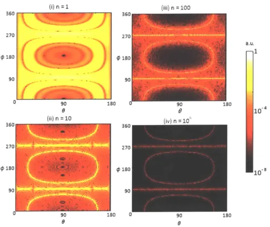
3-1 Radiation intensity profiles at d = 2.5A for varying n. The maximum intensity of the peak is independent of n but the peaks get thinner as we increase n. The location of the peaks depends only on d/A and does not change with n. . . . . 29

3-2 Radiation intensity profiles at A = 100A for varying d, or equivalently varying n = A/2d. . . . . 30

3-3 Several examples of the radiation intensity profile from shaped electron

wavefunctions, which has a sinusoidal profile with periodicity d and 2n = 10 periods in the x direction and Gaussian profiles with width w in both the y and z directions. . . . . 32

3-4 Illustration of the shaped electron wavefunction moving in a periodic force field such as a periodic electric field, an undulator, or a free

electron laser. . . . . 33 3-5 a. Radiation intensity profile for a single point electron travelling at

vo = 0.9c in a periodic field. Radiation within the white dotted line is

blueshifted and outside it is redshifted. b. Radiation intensity profile for a shaped electron wavefunction with n = 10, d = 2.5A/-y travelling at vo = 0.9c in the periodic electric field. c. Radiation frequency profile due to Doppler shift. . . . . 34

3-6 Change in radiation intensity for a shaped electron wavefunction with

n = 10, d = 2.5A travelling at varying vo. Radiation within the white

dotted line is blueshifted and outside it is redshifted. . . . . 35 3-7 Illustration of the shaped electron wavefunction being decelerated by

a uniform electric field. . . . . 37 3-8 Variation of intensity of radiation with photon energy E, and direction

0, for various

#,

emitted by a shaped electron wavefunction with d = 165pm uniformly decelerated for time to = 1.1 x 10-18s. . . . . . 38 3-9 a. Visible radiation in real color (color as it appears to the human

eye) from a single point electron uniformly decelerated for time to =

5 x 10' 6s. b. Visible radiation in real color from the shaped electron

wavefunction with d = 700nm uniformly decelerated for the same to =

5 x 10 -16s. . . . .

. . . .

39

4-1 A shaped electron (superposition of two momentum eigenstates) is

scattered off a nucleus into a single momentum eigenstate and it emits a Bremsstrahlung photon in the process. . . . . 42

4-2 Tree-level Feynman diagrams for Bremsstrahlung. The crosses indicate the Coulomb potential. . . . . 44

5-1 Comparison of differential cross section for an unshaped electron and a shaped electron. . . . . 50 5-2 Heuristic model for amplitudes as a function of detector location. . . 52 5-3 Plots showing a measure of the differential power of photons when

the initial electron state is an superposition state. The letters 'A' through 'E' represent the scenarios of our heuristic model that explain the maxima in the corresponding energy range. . . . . 54 5-4 Plots showing a measure of the differential power of photons when we

incoherently sum over two electron momentum eigenstates. . . . . 55 5-5 Plots showing integral cross section as a function of normalized photon

energy. . . . . 57 5-6 Comparison of differential cross section between a shaped electron

wavefunction with = -r/2 and a incoherent sum over the same

Chapter 1

Introduction

1.1

Motivation

The interaction of free electrons with light is a phenomenon that is ubiquitous in fundamental electrodynamics and also in the development of light sources and ac-celerator technologies. An important class of these interactions is spontaneous emis-sion by a free electron, which takes many guises such as Cerenkov radiation, transi-tion radiatransi-tion, Smith-Purcell radiatransi-tion, Bremsstrahlung, inverse Compton scattering, undulator and synchrotron radiation. These processes have important applications in particle detection, astrophysics, materials characterization, and high-energy light sources [6, 10, 24, 28].

Despite the great variety of the physics and applications of these emission pro-cesses, there are a few common features of these spontaneous emission processes. For example, many of these processes can be well-understood classically [14]. In such a treatment, the electron is described by some time-dependent classical current which radiates into the optical surroundings [16]. As is well known, the expressions for the emitted power derived classically achieve excellent agreement with what is observed barring situations in which the electron recoils heavily from its light emission. What is also fairly well known is that these calculations match a quantum treatment [10, 11]. In a quantum treatment, the light emission is captured as a transition between an initial electron state with no photons and a final state with a scattered electron and

an emitted photon. In such a treatment, it must be assumed either that the initial electron is in a single eigenstate or that its density matrix is purely diagonal. This must be the case because electron superposition states are inherently non-classical.

It follows from this discussion that it is interesting to ask: is it possible to tailor the properties of radiation from accelerated electrons by manipulating their quantum wavefunction? If so, this would be attractive given the recently expanded ability to shape electron wavefunctions into complex spatiotemporal patterns [1, 4, 7, 9, 13, 18,

19, 22, 23, 27, 30, 31, 32]; one could envision designing a partial spacetime profile of

the electron wavefunction in order to achieve a target spacetime intensity profile for the emitted light. On one hand, this question can seem as if the answer is a trivial 'yes' because shaping the electron wavefunction shapes the charge and current density, which classically has a clear effect on radiation. On the other hand, when spontaneous emission happens, it is sensitive to transition current densities and the emission into different final states is incoherent meaning that there are some incoherent aspects of the process. And in fact, there are known cases in which the spontaneous emission power is utterly independent of the initial electron wavefunction. For example, when one considers Cerenkov radiation by an electron superposition, one finds that the long time radiation dynamics are independent of the initial electron wavefunction for reasons of momentum conservation [17]. Thus, the question still remains: to what

extent can one shape radiation by shaping the electron wavefunction?

1.2

Thesis Structure

The thesis can be largely broken into two segments. The first segment uses a semi-classical formalism wherein the Poynting vector from an accelerated charge density is used to demonstrate the non-trivial effects of shaping. The second segment uses a QED formalism wherein the scattering cross section is used to establish a similar claim but from a relativistic quantum field theoretic perspective.

In chapter 2, we develop a semi-classical formalism to describe the radiation from a shaped electron wavefunction. We calculate the Poynting vector for a one-dimensional

sinusoidal charge density that oscillates harmonically at non-relativistic speeds. The time-averaged Poynting vector is calculated in the far-field limit, and it determines the energy being radiated per unit solid angle. In chapter 3, we examine the radiation from the harmonically oscillating sinusoidal charge density in detail. We also show that similar results hold for other spatially periodic charge densities. This formal-ism is then used to show how undulator radiation can be made more directional by shaping the electron wavefunction. Furthermore, we show that shaping the wave-function can make radiation from rapidly decelerating electron more directional and monochromatic.

In chapter 4, we develop a formalism using spinor QED to calculate the differential cross section of an electron superposition state being scattered off a Coulomb potential and emitting a photon in the process. In chapter 5, this formalism is used to show that shaping affects the radiation non-trivially. We demonstrate that the radiation from electron superposition state is distinct from the radiation obtained by summing over the initial electron states incoherently by studying the differential and integral cross sections. We also develop a heuristic model to explain the features seen in these cross sections. In chapter 6, we compare the two approaches, summarize the main results, and propose potential applications.

Chapter 2

Semi-classical Formalism

In this chapter, we develop a semi-classical formalism for describing radiation from shaped electron wavefunctions. We first show that the shaping the wavefunction affects the charge and current density. These charge and current densities are then treated classically.

We consider a particular case of a harmonically oscillating electron wavefunction that has a sinusoidal probability density/charge density in the non-relativistic limit. In classical electrodynamics, the radiation pattern from this setup is described by the Poynting vector in the far-field limit. The physical features of this radiation pattern and its applications to undulator radiation and Bremsstrahlung are studied in the next chapter.

2.1

Charge and Current Densities

In this section, we relate the quantum mechanical wavefunction to the classical charge and current densities. A classical electrodynamic approach would then be used in the following sections to obtain the power radiated by these charge and current densities. It is a well-established fact that time-dependent Schrddinger equation governs the time evolution of any system in quantum mechanics

h2

ao

(t

x)

- V2V(t, x)

+

V(x)O(t, x) =

ih

(2.1)

where 0(t, x) is the quantum mechanical wavefunction, h is reduced Planck's constant,

m. is the mass of the particle, and t and x are the time and position respectively.

In case V(x) = 0, the charge density and current densities are given in terms of the wavefunction by p(t, x) = q *(t, x),0 (t, x) (2.2) and hq (0*(t, x)Vk(t, x) - Vo*(t, x)o(t, x) J(t, x) = 2i xt)tx)(2.3) mn 2i

respectively, where q is the charge of the particle.

These charge and current densities act as sources of electromagnetic fields in the framework of classical electrodynamics. Although we use the Schrddinger equation to generate these currents and resulting fields, our results would be identical even if we used the Dirac equation to describe the dynamics. Note that the Dirac equation

is

ih-yD'I'XP(x) - mcT(x) = 0, (2.4)

where -y" are the gamma matrices, and c is the speed of light in vacuum. In this case, the corresponding four-vector current density is

j"(x)

- TI(x>)y0QP"F(x). (2.5)

The results from Schr6dinger equation and Dirac equation are identical because we always Lorentz transform to a frame of reference where the shaped electron wave-function moves non-relativistically. This can be done without loss of generality; to obtain the radiation in the lab frame, we can simply invert the Lorentz transform after performing the calculations in the electron's approximate rest frame.

Our calculations rely on the central assumption that the magnitude of the charge and current are not significantly modified by the emission of radiation. This is true as long as the energy being radiated by the electron is much smaller than the total energy of the electron i.e., we are neglecting radiation reaction effects. We will show in the following section that by appropriately shaping the wavefunction, the radiation

becomes more directional and energy being radiated can always satisfy this criterion. Hence, the assumption that radiation reaction is negligible is justified.

2.2

Radiation from Harmonically Oscillating

Elec-tron Wavefunction

We will assume that the shaped electron wavefunction generates a line charge with charge density

p(x) = po sin2 _f

2(y)f3(z) - nd < x < nd (2.6)

where d is the periodicity of the electron wavefunction, 2n is the number of periods (or peaks) of the charge density, and

fi(.)

and are arbitrary normalized functions with width much less than d (for instance, they can be 6-functions). Such a periodic charge density can be experimentally realized through either double-slit interference experiments, biprisms [29], or masks [26, 27] with coherence lengths as large as several microns.

Now, this line charge is placed in an oscillating electric field with angular frequency

w i.e.,

Eex(t, x) = Eo sin(wt)i. (2.7)

This scenario is shown in Fig. 2-1.

Since both the mass and charge density are proportional to

I4)(t,

x) 12, all points on the line charge have the same acceleration given by

a(t, x) = ao sin(wt)i (2.8)

where ao = qEo/m is the acceleration amplitude. Thus, the line charge does not

undergo any deformation.

The condition that the charge density does not undergo any deformation is another central assumption our calculations rely on. For the charge density in (2.6), this

(*jxjP) = - sin(wt) 2 (02 z /I A

'I

Itt/p

pit

1l

12

7t

I I

tip

t

Figure 2-1: Illustration of the shaped electron wavefunction. Snapshots of the

oscil-lating wavefunction are shown as a function of time. The sinusoidal curves represent

the sinusoidal probability density/charge density along the x-axis.

assumption holds as long as the x-gradient of the external electric field vanishes i.e.,

axEex(t, X) = 0.

(2.9)

Naturally, this accelerated charge density radiates. In classical electrodynamics,

the directional energy flux is given by the Poynting vector

S(t,

x) =

E(t,x)

x

B(t,x)

(2.10)

where E and B are the electric and magnetic fields produced by the charge density,

and yo is the permeability of vacuum.

The electric and magnetic fields due to a moving charge q with position x,(t) and

velocity v,(t) can be calculated from the Lienard-Wiechert potentials [12] to be

E(t,

x) = q '4-7rEo (1 - I3S2)(

-

)6s)

(1 - n. -3s)3

Ix

x,12

+

(( -

n

)Ix

(()

J

c(1 -

n -a,)31X - Xj )

B(t,x)

=

n(tr)

x

E(t,

x)

(2.11)

(2.12)

where EO is the permittivity of vacuum,

tr = t - _______

C

is the retarded time,

n =x - xS(t)

) x - xS(t)I

Assuming that the charge is confined to move in a small volume near the origin, we consider the far-field limit lx

>>

lx,(t)l, so that

Ix

- xs(t)I

l

xi - x* x-(t) + (9(Ix- 2) lxi (2.16) n(t) e nx - xS(t) nx -xs(t) _nO(x|-2). lxi lxi where nx = x/x.

In this limit, the retarded time is given by

t x

- x- x(t) + O(ixi2

_).

_(2.18)

C iil

Furthermore, consider the non-relativistic limit

i/3sl

< 1, so that (2.11) becomes

n lx - xS1

E(t,

x)

~q

47co q_ 47rEo + (A - n)n- 3s cix - xS1 _t (Ws(tr) .

nx)nx

-clxI Os (tr)) (2.19) (2.20)

+

(x-2)

Note that we neglect the higher order terms in

lxi

as they do not contribute to radiation in the far-field limit.

and (2.13)

)3s (t) =

)

(2.14) (2.15) and (2.17)

Defining 3,, (t) to be the component of /3,(t) perpendicular to nr, i.e.

Is

I(t)

-s(tr)

- (1s(tr)

-nx)nx,

(2.21)

we obtain,

E(t, x)

q

' (tr) (2.22)

47rcoclxl

This is the expression for the electric field from a single point charge. In case of a charge distribution that does not extend out to infinity, we have the electric field in the far-field limit

E(t,

x)

41r1c

j

da

p

)3'

t

-

+

(2.23)

where 3S(t) is the common acceleration of the charge density, as required by the non-deformation assumption. Clearly, E(t, x) is perpendicular to nx.

Thus, the Poynting vector is

S(t, x)

~

E(t, x) x

nx

E(t x) (2.24) I'oc -E(t, x)12

n

_(2.25) fLoc =67 _ d px

(

lx

d

)# t--

+

.x2 (2.26) l6lr2

_Eocjxj

2 ]vLLLPA)s

clxi!

This Poynting vector is directed along nx which corresponds to the radially out-ward direction which matches with our intuition for the Poynting vector corresponding to a radiating source.

Now we substitute into this expression the charge density in (2.6), with f2(y) and f3(z) being 6-functions, and the acceleration in (2.8). Using spherical coordinates for

x = (r sin 0 cos

#,

r sin 6 sin#, r cos 0),

Sp2 16 4rd2 sin2 0 sin2 ( nw sin 0 cos ) sin2 Wt - r1 . ( 2

Sl(t, x) ~4P2

( sn)o

nc. (2.27)

(i) d =0.5 X (ii) d= A 360 360 270 270 a. u. 1 P 190 *0180 90 90 0 90 0 90 180 P

-mE)y0.5

Primary Peaks 360 (iii) d = 1.5X (ivd=2.5A 270 270 0 1S0 '0180 10 90 90 93'.0 0 soIS Secondary Peaks

Figure 2-2: Several examples of the radiation intensity profile for the shaped electron wavefunction (with 2n = 10 periods) for different periodicities d. The secondary peaks appear when d = A and spread out towards the primary peaks as we increase

d.

Taking a time-average, we obtain the final expression ITr2aQ2 sin2 9 sin2

(na

_{sinG cos)}

(S(t, x)) r10 302X2CS0 2

nx

(2.28)

2Eoc n2_I 2 _47r2

(d sin cos4) -

(

wdsin _(2.28) where

Q

= pond is the total charge carried by the charge distribution. In case of

radiation from a single electron,

Q

equals the elementary charge e.

An example of the intensity pattern we can get from (2.28) is presented in Fig. 2-2. The intensity profile of an oscillating point charge and a wavefunction that is much wider than the wavelength of the emitted light are shown in Fig. 2-3 for comparison.

360

b.

a.u.

270 270

0180 0.5 0180 0.5

909

0 90 180 0 0 90 180

Figure 2-3: a. Radiation intensity profile for a single point electron. b. Radiation intensity profile for a wide electron wavefunction with width 50A (similar to a uniform line charge). This wavefunction extends along x direction similar to that illustrated in Fig. 2-1. It shows two narrow peaks, without the additional features in Fig. 2-2.

2.3

Underlying Assumptions

Although we have briefly stated the assumptions required to justify our calculations, it is imperative that we explicitly list out these assumptions again for the benefit of the reader.

First and foremost, we assume that the charge and current densities in the absence of any accelerating electromagnetic fields are produced by a stable, non-dispersive solution to Schr6dinger or Dirac equation. Even though, the particular charge and current densities that we use to derive our results may not satisfy this condition, our results hold more generally for charge and current densities as long as they are periodic in space.

We also assume that the accelerating electromagnetic fields do not deform propa-gating the charge density. This is true as long as the relevant spatial gradients of the fields vanish. Also, the charge density is assumed to be moving non-relativistically at

all times.

The Poynting vector is calculated in the far-field limit. This is a standard approx-imation when analyzing radiation in classical electrodynamics [16]. This classical Poynting vector corresponds to the rate of emission of a single photon per unit solid angle in quantum mechanics.

-1

Our classical treatment of radiation is justified as long as the electron does not

recoil on emitting the photon, i.e., the energy of the photon

is

much less than the

electron's kinetic energy. In other words, the electron must behave purely as a classical

Chapter 3

Results from Semi-classical

Formalism

In the previous chapter, we have obtained an expression for the radiation from a har-monically oscillating electron wavefunction with a sinusoidal charge density. In this chapter, we examine the physical features of this radiation pattern. Furthermore, we apply our formalism to tailor radiation from electron beams passing through fields periodic in space (like undulators). Finally, we study the radiation from rapidly decel-erated shaped electrons in both visible and X-ray, showing it can be made directional and monochromatic.

3.1

Physical Features of Radiation from

Oscillat-ing Wavefunction

To understand the physical features of the radiation pattern, we try to determine the directions in terms of (0, 0) coordinates where the time-averaged Poynting vector

(S(t, x)) is maximized. This is done by examining the (0,

#)

coordinates where the

denominator of (2.28) vanishes.

Firstly, we get fixed peaks at 7 r/2 or 900 and = 37r/2 or 270* that have maximal intensity when 0 = -r/2 or 90* i.e. along the and - directions. We name

these maxima primary peaks.

There are other peaks that are given by sin 0 cos

#

= 27rc/wd = A/d in the large

n limit. Here, A is the wavelength of the electromagnetic radiation having frequency w. These also have maximal intensity when 0 =7r/2 or 900. We name these maxima secondary peaks. These peaks as observed only if d > A.

In order to justify that our claim about the location of these peaks is correct we perform a Taylor series expansion around the peaks. For the primary peak at

(0, 0) = (-r/2, r/2) or (7r/2, 37r/2) , defining 60 = 0 - 00 and JO = #S - #o, we obtain

a|Q

2

/d 2 2 \

I(S(t,x))|

~

2 2

1

- 602

-

(-

-2)

j02)

(3.1)

327r 2oc32jX12 ( A2 3

For the secondary peak at (0o,

#o)

= (w/2, cos-1(A/d)) or (w/2, r - cos-1 (A/d)),

defining 60 0 - 00 and 6q = 0 - q0 as earlier, we obtain that

ao2 i 22 2

I(S(t,x))

~327r2oc3n2fX12

₍₄

₈

₁₂

192)

3d A2 q 6 2 2 d2 A2 23d2 _ 17A2

+ 4A 31 -3252) 2 3 d2 72 2 (3 .2)

where we assume d > A. In the large n limit the quartic term in 60 and the quadratic term in 60 ensure that the maxima is located close to (0, 0).

As we increase d or decrease A, the secondary peaks shift towards the primary peaks as seen in Fig. 2-2. Simultaneously, both the primary and secondary peaks become thinner as we increase d/A. In the extreme case d

>>

A, the wavefunction

becomes very wide and the secondary peaks merge with the primary peaks, so just two extremely narrow peaks are seen. This matches up with the radiation from a wide electron wavefunction shown in Fig. 2-3b. We shall exploit these properties of secondary peaks later in the paper to identify potential sources of monochromatic and directional radiation.

The Poynting vector also depends on the number of periods 2n. As Fig.3-1 shows, both the primary and secondary peaks become thinner as we increase n, but the peak intensity does not change. Thus, we expect that the total power decreases with n.

_____ -A i n 1 (iii) n 100 360 360 270 ₂₇₀ a.u. 0 180 0180 90 - - - - 90 0 90 180 0 ₁₈₀ SL9 10 4 36 (i) n=10 30(iv) n=106 360 0 *10

180

1o-5

90 180 0 90 180 6 0

Figure 3-1: Radiation intensity profiles at d = 2.5A for varying n. The maximum

intensity of the peak is independent of n but the peaks get thinner as we increase n. The location of the peaks depends only on d/A and does not change with n.

The Taylor series expansions in (3.1) and (3.2) reveals that the energy contained in the primary peaks falls as n-1 and the energy contained in the secondary peaks falls as n-3/2_{. It is also evident from (2.28) that the background radiation intensity}

falls as n-2. Here, by background we mean all the regions except the peaks. As the total power radiated is a sum of these three leading order terms,

P = Cprimary + Csecondary + Cbackground

(3.3)

n

n3/2

2

in the large n limit.

At large number of periods i.e., n

>>

1, the background intensity is almost zero and

(i) d=0.5A XNO d =2A M vd=5 X 360 360 360 270 -- 270 270 - a.u. 0 o180 ISO 8 280 I. 90 90 0 90 ISO 0 90 180 0

LI180

0 6 00i d=A (Nv)d=3 ' A d=10 X1-360 360 360 270 270 270 IS O 1 980 0 0 18 90 90 90 0 90 180 0 90 980 90 80 S6 e

Figure 3-2: Radiation intensity profiles at A = 100A for varying d, or equivalently

varying n = A/2d.

the electron wavefunction, we are able to make the radiation directional. Furthermore, the total energy that the shaped electron wavefunction loses is much less than that of the point electron, because the wavefunction causes destructive interference along multiple directions, potentially allowing us to create a radiation source which can be sustained over longer distances or times. It is also worth mentioning that with increasing n we get an increasing number of small scale variations in the intensity as seen in Fig. 3-1.

As a general trend, the width of the peaks (in

#)

decreases as we increase the aperture size (the total width of the wavefunction) of an arbitrary wavefunction, consistently with the uncertainty principle for Fourier transforms. In particular for the above calculation, increasing d or increasing n results in an increase in the aperture size A = 2nd, and the peaks become narrower as seen earlier. This is the reason

why for a point electron, which has zero aperture size, the radiation is uniformly distributed in 0.

aper-ture size A. As Fig. 3-2 shows, increasing the periodicity d while maintaining the aperture size constant. As before, the secondary peaks appear when d = A and

spread out towards the primary peaks as we increase d. Also, both the primary and the secondary peaks become narrower as we increase d. The features in background radiation remain unchanged on changing d, but the average background intensity decreases as d increases.

Although we have presented the above calculations for a particular charge den-sity given by (2.6), similar results should follow for any arbitrary charge denden-sity or equivalently any arbitrary shaped electron wavefunction. For example, consider the charge density

PO

2 2tWX2

p(x) 2 sin (7 -e) - nd

<

x

< nd

(3.4)

27rw d

which arises from a wavefunction shaped in all three dimensions.

Assuming that this charge density also has the acceleration given by (2.8), the time-averaged Poynting vector is

r 2_a

_Q

2 _sin2

0 sin2 (nwd sin 0 cos

#)

2(oc

3

n

2

_IX

2 _{47r2 (i4 sin}

₀

_cos

_)-

_sin

Ocos O)3)

W 2 W2

exp 2 (cos2 0

+

sin2

0 cos2

_#)

nx. (3.5)

This radiation pattern is shown in Fig. 3-3. Interestingly, a large width perpen-dicular to the direction of periodicity restricts emission to the j direction (0,

#)

=

(900, 900) and - direction (0,

#)

= (90', 270*). Then, significant emission occurs only when d = A. This enables an appropriately shaped electron wavefunction to

emit monochromatic and directional radiation at a specific wavelength chosen by the periodicity d.

Currently, it is possible to produce oscillating fields with frequencies as high as a hundred gigahertz in capacitors in distributed systems, and beyond that using

tera-360 270 0180 90 0 90 (ii) d =0.5 A w A 360 270 S180-0 180 90 360 270 0 180 90 90 0 (Mv d =)L. w = 360 270 180 90 so 0 360 270 * 180 90 90 0 180

Figure 3-3: Several examples of the radiation intensity profile from shaped electron wavefunctions, which has a sinusoidal profile with periodicity d and 2n = 10 periods

in the x direction and Gaussian profiles with width w in both the y and z directions.

hertz sources or visible lasers. Our formalism is completely scalable to any frequency, and can thus be used to produce radiation in any of the above frequency ranges. Utilizing ways to introduce more rapid oscillations into wavefunctions would allow us to use this method to produce radiation in X-ray regimes. In the next section, we will explore other methods like undulators to obtain high frequency radiation using currently available technology.

3.2

Application to Undulator Radiation

In this section, we use our framework for analyzing the radiation of shaped elec-trons to tailor radiation from electron beams passing through fields periodic in space like those of an undulator in a free electron laser. We show that radiation from an electron passing through these sorts of systems becomes highly collimated and monochromatic as a result of shaping the electron wavefunction. This can improve

B.U.

110-f , -j = A = I' 5 ' 910-6 6 Mv) d=2 A. W=

z a=aosin(27 _{X)2 t}

[+T IFIF IFto

/0

1912

Figure 3-4: Illustration of the shaped electron wavefunction moving in a periodic force field such as a periodic electric field, an undulator, or a free electron laser.

the collimation beyond what is typically obtained from point electrons in undulators. We then present a number of different experimental schemes for generating a source of such monochromatic and collimated radiation.

We pass our shaped electron wavefunction at relativistic velocity v0y through a

region with spatially oscillating fields. In the inertial reference frame moving with velocity v0j, the wavefunction feels a force that oscillates in time. Such a scenario

is shown in Fig. 3-4. Snapshots of the wavefunction at different instants are shown

with coordinate time being depicted by the color of the wavefunction. The sinusoidal

curves in the illustration are representative of the probability density/charge density. Due to length contraction, the characteristic wavelength of the field falls by a factor of -y = 1/N/1 - vo/c2. In this frame, the intensity distribution of radiation is

given by (2.28). The radiation is monochromatic with wavelength A/y, where A is

the spatial periodicity of the fields.

Returning to the lab frame, the radiation is Doppler shifted. The lab frame

radia-tion pattern for an electron wavefuncradia-tion with charge density given by (2.6) travelling at vo = 0.9c in a periodic field. For comparison, the lab frame radiation pattern from

a point electron with the same kinematics is shown in Fig. 3-5a. Furthermore, the Doppler shifted frequency as a function of direction is shown in Fig. 3-5c.

a.

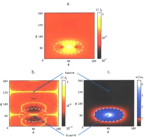
I/Ia 360 1 270 312 0 90 180 107

b.

Redsft C. 360 1 360 4 270 270 3 0 180 *iso .0$1802 2 90 -90 0 90 18 1020 0 0 a Blueshift

Figure 3-5: a. Radiation intensity profile for a single point electron travelling at

7) = 0.9c in a periodic field. Radiation within the white dotted line is blueshifted

and outside it is redshifted. b. Radiation intensity profile for a shaped electron wavefunction with n = 10, d = 2.5A/y travelling at vo = 0.9c in the periodic electric field. c. Radiation frequency profile due to Doppler shift.

~ A/2-y2, which is consistent with the corresponding value for a free electron laser [15]. The Lorentz transform also causes the intensity distribution to shift in toward

the 9 direction as seen in Fig. 3-5b. The secondary peaks come closer to the primary peak along the

y

direction. In short, the radiation along the

Q

direction is both highly intense and maximally blueshifted.

Furthermore, the peak along the

Q

direction becomes stronger, sharper and more blueshifted with the velocity of the electron wavefunction vo as seen in Fig. 3-6. As mentioned earlier, having a large number of periods n makes the peaks even narrower. For cases of very high velocities and large n the background disappears, making the radiation even more monochromatic and directional because the other peak along -y

360 (i - 360 (11) P = U.5c 270 270 - a.u. S180 18 S . 90 93 18D 0- 90 ISO 30(111) VO 0.9c 30(IV) PO 0.99C 10-270 270 0 0 180

Figure 3-6: Change in radiation intensity for a shaped electron wavefunction with

n

=

10, d

=

2.5A travelling at varying vo. Radiation within the white dotted line is

blueshifted and outside it is redshifted.

direction gets maximally redshifted and spreads out. The radiation becomes almost

unidirectional in this case.

The above method can be used to produce radiation in the visible and X-ray

regime. For instance, if electrons at energy 511MeV i.e. -y

=

10' pass through an

undulator with a spatial periodicity A

=

2mm, they emit radiation at A

=

1nm along

the

direction.

Under such conditions, a shaped charge density periodicity of d

=

A, can be

created by interfering two plane waves with an angle 6 ~ 2.4 x 10Orad between their

propagation directions. Similarly, radiation at A

=

0.1nm and A

=

0.01nm requires

6 ~~

2.4 x 10-rad and 6 ~ 2.4 x 10

4

rad respectively at fixed y

=

10', while changing

More generally,

6 ~ 2-yAc/A (3.6)

for relativistic vo. Here, A, is the Compton wavelength of the electron. The above formula holds when assuming d = A. Varying d/A gives us additional control over 6, while only changing the location of the secondary peak (which does not matter for our application of interest since we use the enhancement of the primary peak).

Another method to produce such a charge density is by interfering two plane wavefunctions travelling in the same direction having a small energy difference AE.

In the above example, we need AE ~ 1eV for A = Inm, AE = 10eV for A = 0.lnm or AE ~ 100eV for A = 0.01nm.

More generally,

AE ~ yhc/A (3.7)

for relativistic vo. This requires us to use a different geometry than the one shown in Fig. 3b. In this case, the primary peak is along the direction orthogonal to both the direction of motion of the beam and the direction of acceleration due to the undulator. Note that at such short wavelengths the spatial extent of the wavefunction in all three dimensions needs to be considered because at small enough wavelengths what is normally considered to be a point electron can have a non-negligible width. More generally, the spatial extent of the wavefunction in the y and z directions is important when the width of the wavefunction in these directions is comparable to the wavelength of radiation emitted. Thus, for visible light this corresponds to a width on the order of micrometers and for X-rays this corresponds to a width on the order of angstroms. Hence, for most electron beam sources, the spatial extent in the y and z directions can be approximated as a delta function for visible emission. However, this approximation breaks and the wavefunction's finite width must be considered for X-ray emission. We point the readers to the end of the previous section where an radiation from one such wavefunction -was studied.

This theory can also be applied in a variety of other regimes of parameters, such as in transmission electron microscopes (TEMs). Assuming -y = 1.25 (acceleration

KE = -Eol

+ to

z

xJ~

0

Figure 3-7: Illustration of the shaped electron wavefunction being decelerated by a uniform electric field.

voltage of 127 kV) and d = A, a periodic structure with A = 1.5im corresponds to A = 600nm for AE a 0.6eV or 6 ~ 5.4 x 10-6 rad. Alternatively, one scheme

for generating very narrow wavelength radiation is by sending electrons through an atomic lattice, which, due to the periodicity of the electrostatic fields within them, acts as an electric-field analogue of an undulator, with A = 1 corresponding to A = 40pm for AE ~ 1.62keV or 6 - 0.08rad.

3.3

Application to Bremsstrahlung

In this section, we study the radiation from rapidly decelerated shaped electrons, showing that it can be made directional and monochromatic by tailoring the electron wavefunction. This treatment helps us to deal with Bremsstrahlung and is useful for both visible and X-ray regimes.

Consider a simplified model in which a shaped electron wavefunction, with charge distribution given by (2.6), travels in the i direction. This wavefunction is uniformly decelerated at x = -aoi from t = 0 to t = to. At all other times, the wavefunction is unaccelerated. This scenario is shown in Fig. 3-7. Snapshots of the wavefunction

(i)4# = 0* (ii)

#

= 45' (iii) = 90*

a.u.

24 24 241

18 18 18

yEY EY1 -2

(key) (keV) (keV) 1

12 12 12

6 6 6 0-4

0 90 180 0 90 180 0 90 180

Figure 3-8: Variation of intensity of radiation with photon energy E, and direction 0, for various

4,

emitted by a shaped electron wavefunction with d = 165pm uniformly decelerated for time to = 1.1 x 10-18s.

at different instants are shown with coordinate time being depicted by the color of the wavefunction. The sinusoidal curves in the illustration are representative of the probability density/charge density.

In order to apply our formalism to this case, we first Fourier transform the accel-eration

a(t) = -ao

cj

d.

I

sin ( .2e-) -(t-to/2) (3.8)

Now, each of the Fourier components has its own intensity distribution given by

(2.28) and the total intensity is given by an integral over all Fourier components.

The primary peaks for all frequencies are collocated, so the radiation in the and -Q directions is not monochromatic.

However, the secondary peaks for different frequencies have different locations, so the secondary peaks are split according to their wavelength, creating monochro-matic radiation in each direction. The bandwidth of these peaks depends inversely on n. Thus, shaping the wavefunction provides us with a natural way of making Bremsstrahlung radiation directional and monochromatic.

The radiation from a shaped electron wavefunction is shown in Fig. 3-8. The in-tensity shows bands in frequency because of the coefficients in the Fourier transform of the rectangular pulse. It is evident that the primary peaks for

#

= 900 are collo-cated and attain maximal intensity at 9 = 90* for all photon energies. Furthermore,

a. b. 360 360 270 270 4180 180 90 90 0 90 180 0 90 180 0 0

Figure 3-9: a. Visible radiation in real color (color as it appears to the human eye) from a single point electron uniformly decelerated for time to = 5 x 10- 16s. b.

Visible radiation in real color from the shaped electron wavefunction with d = 700nm uniformly decelerated for the same to

=

5 x 10- 16s.

depending on the photon energy.

Fig. 3-9b shows the radiation pattern (in real color) from an shaped electron wavefunction with periodicity d = 700nm decelerated by a uniform electric field for time to = 5 x 10- 16s. This deceleration time can correspond to an electron moving at

a velocity of 2 x 107m/s passing through a 10nm thick capacitor. The primary peaks

for all frequencies are collocated and they appear white. However, the location of the secondary peaks depends on w, so different frequencies show the secondary peaks at different locations. The radiation is monochromatic at these locations and a rainbow is observed over the visible range. The alternate dark and bright band appear because of the coefficients in the Fourier transform of the rectangular pulse.

For comparison, Fig. 3-9a shows the radiation pattern (in real color) from a point electron undergoing the same deceleration. This radiation is independent of

#

unlike the previous case. Since this radiation is distributed over almost all frequencies, it appears white.

The uniform deceleration required to obtain the aforementioned radiation patterns can be implemented using a capacitor or an atomic potential. To enhance radiation in the visible regime, a deceleration time to ~ 10's is needed, which can be achieved

by passing our wavefunction at a velocity of 107m/s through a capacitor with

capacitors [25], or other modern nanocapacitors [8, 20].

The above treatment can be applied to any arbitrary acceleration or deceleration and we should get similar results. In such a case, the radiation with frequencies up to the inverse timescale of the acceleration is enhanced. This concludes our discussion of the applications that follow from the semi-classical formalism. In the next chapter, we develop a QED formalism to examine the same problem of how shaping the electron wavefunction affects radiation.

Chapter 4

QED Formalism

In this chapter, we develop a QED formalism that describes the radiation from a elec-tron superposition state being scattered off a Coulomb potential. These calculations are a generalization of Bethe and Heitler's original calculations for Bremsstrahlung [2]. In the next chapter, this formalism is used to describe the how superposition affects the radiation being emitted.

4.1

System Description

The system under consideration is shown in Fig. 4-1. An electron is scattered off of the Coulomb potential from a proton fixed in place:

V(x)

=

-

.2

(4.1)

47rco lxl

The initial electron state is taken for simplicity to be an equal probability super-position of two different momenta pi and P2 with relative phase (:

i) = Pi) + e" Ip2) _(4.2)

The momenta are chosen such that

pi

= P21, so that the initial electron state is an energy eigenstate. Also, the angle between pi and P2 is 20j, as shown in Fig. 4-1.

emitted X e - electron incident

I

superposition

e,

Pi electron e- ' k 0Pk Z k l pi) + ei IP2) emitted photon

Figure 4-1: A shaped electron (superposition of two momentum eigenstates) is

scat-tered off a nucleus into a single momentum eigenstate and it emits a Bremsstrahlung

photon in the process.

This initial state

Ii)

makes a quantum mechanical transition into a final state in

which an electron has momentum p' and a photon is emitted with momentum k. We

laabel this final state as If). The photon momentum is parameterized by its frequency

w and its spherical polar angles Ok and

#k,

as illustrated in Fig. 4-1.

These transitions are characterized by the scattering matrix or S-matrix element,

Sp. When squared, multiplied by the photon density of states, and integrated over all

electron momenta, it yields the differential power of photon emission by the electron.

Since the S-matrix is linear, it takes the form

Sfi

-

(S(pi

-

p'k) + ei S(P

2 -+

p'k)) .

(4.3)

Interference will affect the output radiation if cross terms of the squared S-matrix

element integrated over all electron momenta is non-zero. Importantly, the S-matrices carry delta functions expressing energy-momentum conservation. Generally speaking, provided momentum conservation can be satisfied for two different electron momenta

pi and P2 and the same photon momentum k, we expect cross terms to be important.

Because the Coulomb field of the scatterer carries a range of momenta, it is possible for different Coulomb-field momenta qi and q2 to provide the necessary momentum

to bring pi and P2 to the same photon k.

the process described above. Before we commence our calculations, it must be stated

that we will use natural units i.e., h = c = co = 1 from this point onwards.

4.2

Calculations for the S-matrix Element

First consider a simpler process where an electron interacts with the Coulomb po-tential and emits a photon in the process. Let the initial electron have momentum

p and spin s, the final electron have momentum p' and spin s' and the photon have

momentum k and polarization E(k). Let q be the virtual momentum associated with the static Coulomb field.

We are interested in studying the process p -+ p'k. The overlap of the incoming and outgoing states is given by

Out

(p'kjp)j. = lim (p'kle

2iHT TP 44 where H is the QED Hamiltonian and T is the time interval for the process. Now, we define the S-matrix element as

out (p'kIp)n =-5,.,(p --+ p'k). (4.5)

The S-matrix element for this process is of the form

S,,,,(p

-+ p'k)

=

(27r)

4

6(

4)(p - p' -

k

- q) iM,,s,(p -+

p'k)

(4.6)

where M is the scattering amplitude.

At tree level, this scattering amplitude is given by

w Ahere (p har'g(pe) - p'k) t t = ySF(p' + (ie)2k) fy

+-y'SF(p - k) y"] us (p)

c,_,(k) (Ac)

v(q)

(4.7)

q k

p' + k

pp'

Figure 4-2: Tree-level Feynman diagrams the Coulomb potential.

q k

p-k p - k

p P

for Bremsstrahlung. The crosses indicate

are the Dirac matrices, SF(.) is the fermion propagator, and (Ac), is the momentum-space Coulomb potential. This formula follows from the Feynman diagrams shown in

Fig. 4-2.

Let us now put together the various pieces needed to calculate the scattering amplitude. First, we have the momentum-space Coulomb potential is obtained by Fourier transforming the position-space Coulomb potential.

(Ac)v(q)

=

I

Since the position-space Coulomb potential in Coulomb gauge is given by

(Ac)v(x)

=

(

,0,o,00

,

(47rlx

(4.8)

(4.9)

the momentum space Coulomb potential is

(A,),(q)

=

,

Also, the propagators are

SF(p'+

k)

SF(p - k i(/'+ + me) (p' + k)2

-i(PI '++m)

2p' - k ip-4+ Me) _ -+m) -

_{2p k}

(p - k)2 -

me p

0,0,0)

.

(4.10)

(4.11)

(4.12)

d

3x

e

i*,(A,),

(x).

where me is the mass of the electron and

p

=7pp.

Substituting these in (4.7), we get

M ,,,(p -- p'k) -

e

(p') q2

'+ +

me)0 m)(2p' - k - 0(P - P + Me) ()u P - 2p - k I()usp. (4.13)

Substituting (4.6) and (4.13) into (4.3), we can obtain the required S-matrix ele-ment.

4.3

Calculations for Scattering Cross Section

The S-matrix elements can be used to calculate the scattering cross section. As earlier, we start with the simpler process p -+ p'k. The probability of transition is given by

(4.14) Since the normalization factor is

(pp) =

(2ir)32Ep (3)(0)

= 2EpV

(4.15)

where V is the spatial volume of the wavefunction, the scattering probability is

SS'S'(p -- p'k) 12 8EpEpWkV 3 (27r)'6(4)(p - p' - k - q) (')(0) 8EpEp'wkV3 (2r) ()(p - p' - k - q)VT I., 8EpEp'wkV3

Is,'(

p -+ p'k) 12 Vss'(p -+ p'k) 12

.

Thus, the transition probability per unit time is

P

(2,r)46(4)(p - p' - k - q) 2

T

8EpEp-'kV2 _|Mss,(p

-+ p'k).

(4.16) (4.17) (4.18) (4.19) p I out (p'k Ip)i.2 (p Ip)( p' p')(k Ik)

Finally, we have the differential cross section

V )3

du=P

)d3r d3kd3q

(4.20)

(2-F)3 O y

where Op is the speed of the incident electron. Integrating over q using the spatial part of the 6-function,

do

-

1

6(Ep

- - Wk)

d

3

pMd

3

1M

₈,k

,,(p

-+

p'k)1

2

(4.21)

(27r)5 8EpErWkp

Note that this fixes q = p - p' - k as required by momentum conservation. Also, we

have qO = 0 by definition.

Using spherical coordinates,

1 6(E~ - E,- )2

da = I 3

- -pE ,dEpdQ,, w2dwkdQk

IMs,s,(p

-+

p'k)1

2 (4.22)

(27r)5 8EpEp'LWkp fk

where 3p, is the speed of the final electron and dQ denotes an angular element. Integrating over Ep, using the -function,

do =

I

kEpp OdQ

, dwkdQk

IMS,s'(p

-+

pk)

2 (4.23)

2567r5 EPOP(

Till now, we have neglected the electron spins and photon polarizations. To get the total cross section, we average over the initial electron spin, and sum over the

final electron spin and photon polarization to get

1 Wk 73, EP1 (12

do = 2567r5 O7

E

dQo dWkdQk 2 SMS, (p - ' . (4.24)

s( ,eStk)

To obtain the cross section for radiation at a frequency and direction, we integrate over the electron solid angle to get the final expression for the differential cross section for the photon

d= IW2r

_{dQp, E}

_{MIs,p,(p -+}

_p'k)

₁

2

(4.25)

dk -5127w 5 OpEp