HAL Id: hal-01910400
https://hal.inria.fr/hal-01910400
Submitted on 31 Oct 2018
HAL is a multi-disciplinary open access
archive for the deposit and dissemination of
sci-entific research documents, whether they are
pub-lished or not. The documents may come from
teaching and research institutions in France or
abroad, or from public or private research centers.
L’archive ouverte pluridisciplinaire HAL, est
destinée au dépôt et à la diffusion de documents
scientifiques de niveau recherche, publiés ou non,
émanant des établissements d’enseignement et de
recherche français ou étrangers, des laboratoires
publics ou privés.
Population and Individual Patterns
Igor Koval, Jean-Baptiste Schiratti, Alexandre Routier, Michael Bacci, Olivier
Colliot, Stéphanie Allassonnière, Stanley Durrleman
To cite this version:
Igor Koval, Jean-Baptiste Schiratti, Alexandre Routier, Michael Bacci, Olivier Colliot, et al..
Spa-tiotemporal Propagation of the Cortical Atrophy: Population and Individual Patterns. Frontiers in
Neurology, Frontiers, 2018, 9, pp.235. �10.3389/fneur.2018.00235�. �hal-01910400�
doi: 10.3389/fneur.2018.00235
Edited by:
Yasser Iturria Medina, McGill University, Canada
Reviewed by:
Alexandra Young, University College London, United Kingdom Bruno Michel Jedynak, Portland State University, United States
*Correspondence:
Igor Koval igor.koval@icm-institute.org †
Data used in preparation of this article were obtained from the Alzheimer’s Disease Neuroimaging Initiative (ADNI) database (adni.loni.usc.edu). As such, the investigators within the ADNI contributed to the design and implementation of ADNI and/or provided data but did not participate in analysis or writing of this report. A complete listing of ADNI investigators can be found at: http://adni.loni.usc.edu/wp-content/ uploads/how_to_apply/ADNI_ Acknowledgement_List.pdf
Specialty section:
This article was submitted to Neurodegeneration, a section of the journal Frontiers in Neurology
Received: 28 July 2017 Accepted: 26 March 2018 Published: 04 May 2018 Citation:
Koval I, Schiratti J-B, Routier A, Bacci M, Colliot O, Allassonnière S and Durrleman S (2018) Spatiotemporal Propagation of the Cortical Atrophy: Population and Individual Patterns. Front. Neurol. 9:235. doi: 10.3389/fneur.2018.00235
Spatiotemporal Propagation
of the Cortical Atrophy: Population
and Individual Patterns
Igor Koval1,2*, Jean-Baptiste Schiratti1,2, Alexandre Routier1, Michael Bacci1,
Olivier Colliot1,3,4, Stéphanie Allassonnière2and Stanley Durrleman1for the Alzheimer’s
Disease Neuroimaging Initiative†
1Inria Paris-Rocquencourt, INSERM U1127, CNRS UMR 7225, Sorbonne Universités, UPMC Univ Paris 06 UMRS 1127,
Institut du Cerveau et de la Moelle épinière, ICM, Paris, France,2INSERM UMRS 1138, Centre de Recherche des Cordeliers,
Université Paris Descartes, Paris, France,3
AP-HP, Pitié-Salpétriere Hospital, Department of Neurology, Paris, France,
4
AP-HP, Pitié-Salpétriere Hospital, Department of Neuroradiology, Paris, France
Repeated failures in clinical trials for Alzheimer’s disease (AD) have raised a strong interest for the prodromal phase of the disease. A better understanding of the brain alterations during this early phase is crucial to diagnose patients sooner, to estimate an accurate disease stage, and to give a reliable prognosis. According to recent evidence, structural alterations in the brain are likely to be sensitive markers of the disease progression. Neuronal loss translates in specific spatiotemporal patterns of cortical atrophy, starting in the enthorinal cortex and spreading over other cortical regions according to specific propagation pathways. We developed a digital model of the cortical atrophy in the left hemisphere from prodromal to diseased phases, which is built on the temporal alignment and combination of several short-term observation data to reconstruct the long-term history of the disease. The model not only provides a description of the spatiotemporal patterns of cortical atrophy at the group level but also shows the variability of these patterns at the individual level in terms of difference in propagation pathways, speed of propagation, and age at propagation onset. Longitudinal MRI datasets of patients with mild cognitive impairments who converted to AD are used to reconstruct the cortical atrophy propagation across all disease stages. Each observation is considered as a signal spatially distributed on a network, such as the cortical mesh, each cortex location being associated to a node. We consider how the temporal profile of the signal varies across the network nodes. We introduce a statistical mixed-effect model to describe the evolution of the cortex alterations. To ensure a spatiotemporal smooth propagation of the alterations, we introduce a constrain on the propagation signal in the model such that neighboring nodes have similar profiles of the signal changes. Our generative model enables the reconstruction of personalized patterns of the neurodegenerative spread, providing a way to estimate disease progression stages and predict the age at which the disease will be diagnosed. The model shows that, for instance, APOE carriers have a significantly higher pace of cortical atrophy but not earlier atrophy onset.
Keywords: Alzheimer’s disease, cortical atrophy, brain networks, spatiotemporal propagation patterns, individual variability
1. INTRODUCTION
Neuroimaging studies have shown an alteration of the brain struc-ture during the course of Alzheimer’s disease (AD) (1,2). These lesions appear during the prodromal phase of the disease (3–
5) whose observation have been limited due to the absence of clinical symptoms and diagnosis. The importance of the structural changes before the clinical symptoms led to hypothetical models (6), which have been later refined thanks to the gathering of multiple scientific evidences. These modifications took the form of a structural change of the brain in particular an important neuronal loss and an atrophy of the brain cortex (7,8). The study of the temporal evolution of the cerebral cortex reveals an atrophy of the gray matter (9). This cortical atrophy presumably relates the traces of the progression of the lesions over the brain surface. A fine-scale modeling of the atrophy propagation is likely to give a wider understanding of the disease evolution, as the structural markers seems reliable to assess the conversion to the AD stage, potentially carrying subtle indicators of the disease progression in early phases.
The spatiotemporal propagation of these alterations encloses two entangled components. On the one hand, the spatial charac-terization of the lesions over the brain surface at each time, and, on the other hand, a temporal dynamic of these alterations that may differ from one region to another. Characterizing the proper dynamics of these lesions relies on the possibility to reconstruct the whole time-line of AD, at both a spatial and temporal level, out of short-term observations that are not temporally aligned. Another challenging aspect consists in the variability inherent to the individual patterns of atrophy that requires to consistently compare the subject-specific spreads of alterations. Accounting for the interindividual variability in term of lesion propagation should allow to reconstruct individual patterns of propagation, paving the way to possible personalized model of atrophy, that potentially informs on subject-specific age of conversion or dis-ease stage.
Recently, large datasets have opened the opportunity to inves-tigate data-driven models that have refined and validated these hypotheses to some extend, in particular event-based models (10–
12) that considers the propagation as a series of events, allowing to define a sequence of disease stages. They characterize the overall variability of the events ordering at a population level. However, these models are not well suited to relate for the temporal delays of the alterations at a population level, neither to determine individ-ual cortical atrophy. Multimodal observations, including positron emission tomography (PET) scans, magnetic resonance imaging (MRI) and biomarkers, have been gathered within longitudinal databases, i.e., repeated observations of patients during significant periods of time. The underlying intention is to provide multiple individual snapshots of the disease—patients examined during short-term periods—in order to reconstruct the long-term history of the pathology (13,14) at a group and individual level. Moreover, it offers the possibility to describe and interpret the observed data contrary to quantiles or percentiles that require arbitrary reference distributions. A challenging aspect of AD patient comparison is the fact that, even though AD is related to age, the latter is not a good proxy of the disease stage (15–17) leaving us without any
easy way to align all the individual on the same time-line. In Ref. (18), the authors introduced mixed-effect model that consider each individual trajectory as a variation of a mean scenario of evolution, with a time-warp function that is able to realign the subjects on the same time-line (19). It allows to characterize a spatial and temporal variability of propagation in the sense that it defines a group-average trajectory of propagation with the possibility to reconstruct individual observations thanks to per-sonalized parameters. Nevertheless (18), constrain the model to parallel profiles of progression which does not hold when looking at signals that have various dynamics. Moreover, the model does not take into account the spatial correlations between the data whereas (17), which focus on spatiotemporal patterns of progres-sion for images, exhibited that this led, in the case of a non-linear mixed-effects model, to poor estimations of the subject-specific parameters and individual trajectories.
To account for the spatial structure of the signal, networks have been introduced (20, 21), representing the brain areas as the graph nodes. In this paper, the networks correspond to a graph representation of a signal spatially distributed, namely, the cortical thickness mapped on a mesh representation of the cortex. The node values are the cortical thickness values over time on the related brain area. Extracting and projecting patients cortical thickness on the common mesh allows to compare their atrophy on the same atlas to exhibit similar patterns. As we expect the signal propagation to be spatially smooth with a similar temporal profile of change for neighbor nodes, we consider that a subset of the graph nodes act as control nodes. They define an evaluation function such that the signal at each node is an interpolation of the signal at the control nodes, enabling to smooth the high frequencies (22). The proximity between nodes is defined by the distance matrix which informs on the distance between any pair. Moreover, the number of nodes of this vertex-based graph can be tuned based on the desired application, potentially the same as the resolution of the input data, e.g., a voxel for MRI or PET data.
The aim of this paper is to introduce a model of the cortical atro-phy propagation during the long-term course of AD thanks to a graph representation of the neuroimaging data. This model is able to personalize the reconstruction of the propagation to individual longitudinal measurements, allowing to describe the stages of the disease, potentially in the future. The model is described as a gen-eral framework for any longitudinal data spatially distributed on a common graph and it is instantiated to exhibit the propagation of the cortical atrophy on the left hemisphere of the brain, across nearly 2000 regions, thanks to longitudinal observations of 154 mild cognitive impaired (MCI) patients that were later diagnosed with AD. While exhibiting an average pattern of propagation, this mixed-effects model allows to reconstruct individual observations through time.
2. MATERIALS AND METHODS
2.1. Sketch of the Method
Prior to detail our method, we would like to sketch the key ideas and notations of our work to ease and guide the reading. First, we consider I patients; each patient i is observed Jitimes, his jth visit
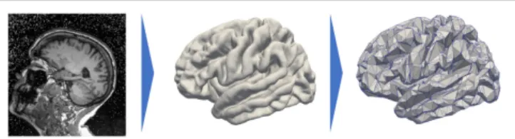
being at age tij, and each observation led to an MRI scan as shown on the left hand side of Figure 1. Segmentation of the cortical thickness, out of the neuroimaging observations, are mapped onto a mesh, as presented on the middle part of Figure 1. The last step corresponds to a subsampling process that led to a graph G of K nodes, characterized by a distance matrix D. At each node, the individual observations define a time-series describing the evolution of the signal through time.
In a second time, we assume that, at each node k of the graph G, there exists a function t7→ γk(t) that describes a characteristic evo-lution of the signal at this node, as shown on Figure 2. The time-series of individual i at node k derives from a continuous function
ηik(t), which is assumed to be a spatial and temporal variations of the representative trajectory γk(t), illustrated on Figure 3. The temporal variation corresponds to the time realignment of individual i on the common time-line. It adjusts the individual dynamics to a mean pace of evolution, thanks to personalized parameters τiand αi. τistands for the individual time-shift to the mean disease onset, allowing an early (τi<0) or delayed (τi<0) age at diagnosis. The parameter αiintegrates the patient-specific possibility to have a faster (αi>1) or slower (αI<1) pace of atro-phy compared to the mean scenario of changes. On the other side, the spatial variation corresponds to the adjustment from the mean cortical thickness to individual data. It accounts, for instance, for the difference in size or in spatial thickness distribution at the same disease stage.
We consider that the characteristic signal γk(t) at node k belongs to a family of curve, here the straight line curves, parametrized by the cortical thickness pkand the rate of atrophy
vk. To account for the spatial structure of the signal and the large number of nodes, a subset of nodes, referred to as control nodes, is selected to control the interpolation of the cortical and atrophy values over all the nodes. The distribution of the control nodes depends on the size of the kernel bandwidth such that the kernels densities map almost uniformly the feature space.
FIGURE 1|Data preprocessing that projects the cortical thickness of the raw MRI observation (left) on a mesh, namely, the FSAverage atlas constituted of 163.842 nodes per hemisphere (middle) before subsampling it and averaging the signal onto a 1,827-node graph (right).
The model introduces population parameters, that allow to define a characteristic spatiotemporal trajectory of the atrophy, and individual parameters, that not only enable to reconstruct individual trajectories but also permit the statistical study of the distribution of spatiotemporal atrophy patterns. These parameters are estimated thanks to the Monte-Carlo Markov-Chain Stochas-tic Approximation Expectation-Maximization (MCMC-SAEM) algorithm, which handles non-linear mixed-effects models, with theoretical guarantees and consistent results in practice.
2.2. Subjects and Data Preprocessing
Data used in the preparation of this article were obtained from the Alzheimer’s Disease Neuroimaging Initiative (ADNI) database (adni.loni.usc.edu). The ADNI was launched in 2003 as a pub-lic–private partnership, led by Principal Investigator Michael W. Weiner, MD. The primary goal of ADNI has been to test whether serial magnetic resonance imaging (MRI), positron emis-sion tomography (PET), other biological markers, and clinical and neuropsychological assessment can be combined to measure the progression of mild cognitive impairment (MCI) and early Alzheimer’s disease (AD). For up-to-date information, see www. adni-info.org.The Alzheimer’s Disease Neuroimaging Initiative (ADNI) dataset contains longitudinal MRI data for patients that are, at each visit, either cognitively normal (CN), mild cognitive impaired (MCI) patients, or, AD subjects. We selected all the subjects that presented a monotonous decline from MCI to AD, called the MCI converters, removing those that may convert from AD back to MCI or CN. Although AD patients get through an MCI phase, we could not keep CN to MCI patients as they might just as well convert to another dementia. Also, the patients that underwent from CN to MCI and then to AD are not numerous enough to give robust estimation of early stages (CN to MCI). Thus, we kept only the MCI to AD visits of such patients. Alto-gether, the paper focuses on 154 MCI patients that represents 787 visits, each individual being examined 5 times on average, from 2 to 7 times.
Each visit led to a T1-weighted MRI acquisition, as shown on the left side of Figure 1. The longitudinal pipeline of FreeSurfer (23) was used to extract the cortical thickness of the left hemi-sphere of the brain which was then projected on a common atlas, namely, FSAverage (24), which is a three-dimensional mesh composed of 163,842 nodes for each hemisphere represented on the central part of Figure 1. This common fixed-graph allows to compare the cortical thickness between visits or patients, node to node.
FIGURE 2|Mesh of the cortical surface where each node embeds a time-series of observations (red points). At node k, the function γk(t), which can be
FIGURE 3|Geometric description of the construction of the mean and individual spatiotemporal trajectories in the space of measurement, which is the Riemannian Manifold M that embeds both the real observations and the trajectories. (A) Three-dimensional space embedding individual observations (blue points) of two individuals and the mean spatiotemporal trajectory γ0(red curve). (B) The spatial variations from the group-average trajectory γ0to the individual observations are captured in individual vectors wiand wj, called space shifts. (C) The vector wiis parallel-transported along γ0(orange vectors) to define a parallel curve ηithat
characterizes the individual spatiotemporal trajectory.
The data acquisition and interindividual alignment led to a considerable noise, especially in terms of variability in the mea-sures for close nodes. To smooth this noise and to reduce the computational time, we subsampled the initial graph into a new graph of 1,827 nodes. To do so, we selected 1,827 nodes uniformly distributed over the whole FSAverage graph; the other nodes were then associated to one of the 1,827 nodes thanks to a geodesic distance d on the graph (i.e., the length of the shortest path on the surface mesh between the nodes) using the Fast Marching Algorithm on the mesh (25). Therefore, it constitutes collection of nodes referred to as patches. The value of each node of the subsampled graph is the average value over the corresponding patch, each being constituted of approximately 89 initial nodes of the FSAverage graph. The resolution of this vertex-based approach is lower than the initial one, shown on the right hand side of
Figure 1, but still holds the brain topology while smoothing part
of the acquisition noise. In our case, each observation can be considered as a vector of size 1,827 where the kth coordinate is related to the kth node of the common fixed-graph G. The latter is also described by the distance matrix D between the 1,827 nodes. It was obtained using the geodesic distance d between the 1,827 nodes on the initial graph FSAverage, whose edges are weighted by a physical length. Finally, for all i, j∈ {1, . . . , 1,827}, we set
Dij=d(xi, xj) where xiand xjare two nodes of the graph. In the following, we will present a data-driven model which allow to track the propagation of any signal spatially distributed, supposedly the cortical thickness. We consider a longitudinal dataset y = (yi,j)1≤ i ≤ I, 1 ≤ j ≤ Jiof I individuals, each patient
i being observed Jitimes during the study at ages (tij)1≤ j ≤ Ji. We suppose that there exist a common fixed-graph G defined by a setV = (x1, . . . , xK) of K nodes and a distance matrix D which accounts for the distance between the nodes. Any node xk∈ R3 corresponds to a coordinate of a point in space. Each observation
yij= =(yij1, . . . , yijK)∈ Rk corresponds to the measured signal spatially distributed over the N nodes of G, represented by a point in the multivariate spaceRk, schematically represented on
Figure 3A for K = 3, as if there were only 3 vertices in the mesh.
Therefore, it defines a network whose nodes are valued with the signal of interest. It follows that the collection (yij)1≤ j ≤ Jiof the
observations of a particular subject defines a network that embeds a time-series on each node of G, indexed by the patient age at each observation (tij)1≤ j ≤ Ji.
2.3. Model
2.3.1. From Short-Term Data to Long-Term History We assume there that the repeated observations of a subject are sampled from a continuous function t7→ ηi(t) = (ηi1(t), . . . , ηiN (t)), where ηik(t) describes the decrease of cortical thickness of this
ith individual at vertex k, such that
∀ i ∈ {1, . . . , I} ∀ j ∈ {1, . . . , Ji} ∀ k ∈ {1, . . . , K}
yijk= ηik(tij) + ϵijk, (1)
where ϵijk ∼ N(0, σ2)corresponds to the model noise, whose variance is σ2.
The function t7→ ηik(t) describes the evolution of the time-series at node k for the individual i. Thus, the vector function
t7→ ηi(t) = (ηi1(t), . . . , ηiN(t)) describes the continuous evolu-tion on the graph for a particular individual, i.e., the spatiotempo-ral propagation of the signal over the whole brain. It corresponds to a spatiotemporal trajectory in the space of measurements. The trajectory t7→ ηi (t) is therefore able to reconstruct the existing observations (yij)1≤ j ≤ Ji, defined at the related time-points (tij)1≤ j ≤ Ji, as shown on Figure 3B, but also generate an observation at any time t, potentially in the future.
The repeated data of each individual is a particular window in the long-term course of the disease that potentially overlaps with other patients. We aim to realign along a common time-line these short-term sequences by carefully analyzing the spatiotemporal patterns within each short-term snapshot. Nevertheless, to do so, we also need to account for the interindividual variability in corti-cal thickness measurements and trajectories of propagation across the network. The interindividual variability prevents us from con-sidering any individual propagation as a good representation of the disease evolution.
Consequently, we assume that there exists a mean scenario of propagation, defined by a group-average spatiotemporal trajec-tory t7→ γ0(t), represented on Figure 3C, such that each
mean scenario of changes, detailed in section 2.3.2. This typical scenario of change describes the mean pattern of spatiotemporal propagation of the signal and writes γ0(t) = (γ1(t), . . .,γK(t)) where for all k ∈ {1,. . ., K}, t 7→ γk(t) characterize the typical temporal evolution of the cortical thickness on the brain region related to the node k. As represented in Figure 2, each node has a different temporal profile of atrophy, accounting for the variation of the cortical thickness over time.
2.3.2. Individual Estimation
Translating the generic framework introduced by Schiratti et al. (18) into this case requires to exhibit individual parameters that characterize the individual spatial and temporal variations to the mean, namely the space shifting and the time reparametrization. 2.3.2.1. Time Reparametrization
We introduce a time-warp function ψi(t) that corresponds to a time reparametrization that adjust the individual dynamics on a common time-line, which here is the average spatiotemporal trajectory γ0. For any patient i with observations (yij)1≤ j ≤ Jiat time-points (tij)1≤ j ≤ Ji, ψi(tij) = αi(tij–t0–τi) + t0 where t0 is a
common reference time of the reparametrization, αiencodes for the individual pace of propagation and t0+ τidescribes subject-specific time-shift to the mean disease onset. As such, if the acceleration factor αiis greater than 1, it corresponds to a faster
pace of cortical atrophy whereas αi<1 indicates a slower pace
of atrophy. In the same way, the larger the value of the time-shift τiis, the later the disease occurs. Therefore, it leads to write
ηi(t) = γ0(ψi(t)) + εij. It adjusts the pace at which the trajectory is followed for the ith individual.
2.3.2.2. Space Shifting
In the space of measurementsRK, we consider individual obser-vations and the mean trajectory γ0(t) as shown in Figure 3A.
In order to account for the spatial variability of the individual trajectories, we assume that there exists, for any individual i, a vector wi∈ RKcalled the space shift, that characterizes the spatial variations from γ0(t) to the observations as shown in Figure 3B.
For any point on γ0(t), γ0(t) + wiis assumed to be on the
individ-ual trajectory. Therefore, it is possible to translate all the points (γ0(t))t ϵRto (γ0+ wi)t ϵRas shown in Figure 3C. This collection
defines the individual trajectory ηi(t). This space shift must be orthogonal to the trajectory as it ensures the identifiability of the model. In fact, if the direction wiwas not orthogonal to the trajectory, then the projection of wi on the geodesic γ0 would
interfere with the individual time realignment induced by the dynamic parameters (αi,τi).
Using mathematical tools from the Riemannian geometry beyond the scope of this study (26) shows that the kth coordi-nate of the individual spatiotemporal trajectory writes ηik(t) =
γk(γ˙kw(ikt0)+ ψi(t)). As the space shift must be estimated inR
K, w i is supposed to be a linear combination of few independent com-ponents, in the spirit of independent component analysis (ICA) (27). It leads to consider A a K× Ns matrix of Ns independent directions, and (sij)1≤ i ≤ I, 1 ≤ j ≤ Nsparameters to estimate. si = (si1, . . . ,siNs)∈ R
Nscorrespond to parameters of individual i that characterize his spatial variations from the mean spatiotemporal
trajectory. The orthogonality condition, mentionned in the pre-vious paragraph, leads to consider a basis (B1, . . . ,B(K−1)Ns)of matrices, whose columns are orthogonal to the direction of γ0(t),
and parameters (βl)1≤ l ≤ (K–1)Nssuch that A = ∑(j=1K−1)Ns βjBj. This procedure allows to reduce the dimension of the parameters to estimate for each wi, from K to the chosen number of sources.
It leads to write: yijk= γk ( wik ˙γk(t0)+ αi(tij− τi− t0) +t0 ) + εijk. (2) 2.3.3. Curve Parametrization
In this paper, we consider a straight line model such that
γk(t) = vk(t–tk) + pk, vkaccounting for the ratio of atrophy and pk for the thickness value at time tk. A linear decay in cortical atrophy is then represented by a straight line trajectory, parametrized by time, in the K-dimensional space as shown on Figure 3. Note that as shown on Figure 2, it is possible to parametrize the same curve with two distinct sets (p1, t1) and (p2, t2) preventing from
having an identifiable model. We decided to fix the parameter
tk among all the nodes such that for all k ∈ {1,. . .,K} tk=t0,
the time reference used in section 2.3.2.1, without any loss of generality as t7→ γk(t) is defined onR. Despite the linear form of each coordinate t7→ γk(t), the resulting model is non-linear as it includes among others, multiplication of individual and population parameters.
Finally, equation (2) becomes
yijk=pk+wik+vkαi(tij− τi− t0) + εijk. (3) This model therefore defines a distribution of multivariate straight line trajectories that accounts for the distribution of the individual trajectories.
2.3.4. Spatial Smoothness
The model proposed in this paper deals with data that are spatially distributed on a graph G defined by a set of nodesV = (x1,. . ., xK), where each node embeds a spatial coordinate inR3. We expect a smoothly varying profile of atrophy across nodes. The proximity between edges is given by the distance matrix D.
In order to ensure small variations of the signal, we introduce a subsetVc= (xd1, . . . ,xdNc)⊂ V whose vertices are called control nodes. Instead of estimating (pk)1≤ k ≤ K(resp. (vk)1≤ k ≤ K) at all the nodes, we consider only the parameters at the control nodes (pdk)1≤k≤Nc(resp. (vdk)1≤k≤Nc). We introduce a estimation func-tion x7→ p(x) (resp. x 7→ v(x)) for all x ∈ V such that, at the control nodes, the function is equal to the parameters:∀k ∈ {1,. . .,Nc},
p(xdk) =p
dk(resp. v(x dk) =v
dk). At the other nodes, the function is an interpolation of the parameter value at the control nodes weighted by the distance to each of them. Therefore, the control vertices control the evaluation of the parameters among all the nodes.
We choose a Gaussian kernel Kb as interpolation splines:
∀ x, y ∈ V, Kb(x, y) = exp(−d(x,y)
2
b2 )where d is the geodesic
distance on the mesh and b is the kernel bandwidth. This interpo-lation allows to remove the possible high frequencies, smoothing
the signal spatially. Therefore, it leads to write: ∀ x ∈ V, p(x) = Nc ∑ i=1 βpiKb(x, xdi) and ∀ x ∈ V, v(x) = Nc ∑ i=1 βivKb(x, xdi). (4)
The parameters (βpi)1≤i≤N
c (resp.(β i
v)1≤i≤Nc) are the solution of the linear system pdk = ∑Nc
i=1β i pKb(xdk,xdi)(resp. v dk = ∑Nc i=1βviKb(xdk,xdi)).
Given these interpolations, equation (3) writes
yijk=p(xk) + (Asi)k+v(xk)αi(tij− τi− t0) + εijk. (5) Even though the distance computed for the cortical thickness corresponds to a distance on the brain cortex, it is possible to compute a connectivity distance based on the connectome, or even an appropriate combination of some of these distances. The challenging part is to put into correspondence areas defined by the connectivity matrices and other networks such as the FSAverage Atlas.
The choice of the setVcof control nodes among the whole set of nodesV is mostly determined by the choice of the bandwidth
b: their uniform distribution is such that there is an approximate
distance b between them. In the case of the cortical thickness, we have chosen a bandwidth equal to 16 mm which is representative of the spatial variability of the signal.
2.4. Algorithm
Equation (5) describes a mixed-effects model, introducing population and individual parameter in this high-dimensional non-linear model. We consider that ((αi)1≤i≤I, (τ )1≤i≤i, (sij)1≤i≤pI,1≤j≤Ns) are random-effects of the model, leading to write∀ i ∈ {1,. . ., I} ∀j ∈ {1,. . ., Ns}: αi=exp(ξi) , ξi∼ N (0, σξ2), τi∼ N (0, σ2τ), and, sij∼ Laplace ( 0,1 2 ) . (6)
αicorresponds to the realization of a log-normal distribution so that it is always positive, preventing the individuals to present an increasing cortical thickness over time. Moreover, the Laplacian distribution of sijarises from theoretical considerations as we need the model to be identifiable, i.e., the solution of the problem to be unique. Finally, these random-effects account for the statis-tical distribution of the individual trajectories. In the following, we consider z = ((αi)1≤ i ≤ I, (τ )1≤ i ≤ I, (sij)1≤ i ≤ I, 1 ≤ i ≤ Ns) as hidden variables.
Given equation (5) and the observations y, we would like to estimate the parameters θ = (t0, (pdk)1≤k≤Nc, (vdk)1≤k≤Nc,
(βk)1≤k≤Ns(K−1), στ, σξ, σ)as a maximum likelihood estimate (MLE) θ * = argmax p(y|θ). The natural way to perform such esti-mation in mixed-effects models is the Expectation-Maximization algorithm (28). Unfortunately, the E-step is intractable and it is not possible to sample according to the conditional distribution
ALGORITHM 1 | Estimation of the general and individual cortical thickness decrease with the MCMC-SAEM algorithm.
Input: Longitudinal dataset y = (yi,j)i, jof measurement maps, with the
corresponding ages (ti,j)i, j.
Initial parameters θ0and latent variables z0. Geometrically decreasing sequence of step-sizes ρk.
Sufficient statistics Sk Initialization: set k = 0 and S0=S(z0).
repeat
Simulation: foreach block of latent variables zbdo
Draw a candidate zc b∼ pb(.|zkb). Set zc=(zk+1 1 , . . . ,zk+1b-1,zcb,zkb+1, . . . ,zknb ) . Compute the acceptation ratio ω = min
[ 1,q ( zc|y,θk) q(zk|y,θk) ] . end Stochastic approx.: Sk+1← Sk+ ρk[S(zk+1)− Sk]. Maximization: θk+1← θ∗(Sk+1). Increment: set k← k + 1. until convergence; output: Estimation of θ*.
Samples (zs)sapproximately distributed following q(z|y,θ∗).
p(z|y, θ). Therefore, we use a stochastic version of the EM
algorithm coupled with a Monte-Carlo Markov-Chain method, namely, the Monte-Carlo Markov-Chain Stochastic Approxima-tion ExpectaApproxima-tion-MaximizaApproxima-tion (MCMC-SAEM) algorithm that is able to deal with non-linear equations in a high-dimensional setting. The algorithm is proven to convergence (29) if the model belongs to the exponential family. In our case, it cor-responds to consider that pdk∼ N (p, σ2
p), vdk∼ N (v, σv2) and
βk∼ N (βk, σ2β).
This leads to consider z = ((ξi)1≤i≤I, (τi)1≤i≤I, (si)1≤i≤I, (pdk)
1≤k≤Nc, (v dk)
1≤k≤Nc, (βk)1≤k≤Ns(K−1)) as the extended hidden variables and θ = (t0,p, v, (βk)1≤k≤Ns(K−1), σξ, στ,
σp, σv, σ)as the parameters of the model. The latter introduces sufficient statistics S of the model that are functions of the observations y and latent variables z. The aim of such functions is to disentangle the maximization of the parameters θ and the simulation of the latent variables z.
The pseudo-code of the algorithm, reproduced in Algorithm 1, shows the different steps of the optimization until convergence. For further information about the steps of the algorithm, the reader is referred to Ref. (29–31) and references therein.
2.5. Simulation Study
Since we introduce a new approach to deal with longitudinal data spatially distributed, we performed a simulation procedure to show both the legitimacy of the model used, and the effective-ness of the estimation procedure. To this end, we define a graph represented on the top left of Figure 4, representing a square mesh of 7 nodes per edge, thus 49 nodes in total. Among them, 9 equally distributed nodes represent the control nodes, in red on the figure. As we simulate data according to equation (3), we choose position and velocities across the node of the graph, as shown on the top right part of Figure 4. Then we simulated realizations (ξi,τi, (sij)1≤ j≤ Ns)1≤ i ≤ Nfor 350 patients, from 4 to 12 visits each (2,980 visits in total) such that it represents 350 longitudinal trajectories of biomarkers spatially distributed. These
FIGURE 4|Simulation study performed to show the effectiveness of the parameter estimation procedure. The upper part describes the simulated graph (left) and the true velocities across the nodes (right). On the bottom part, a convergence example is given (left) as well as the estimated velocities estimated across the graph (right).
TABLE 1|The table shows the ability of the algorithm to estimate the real value of the model parameters.
Parameter Initial Final value Real value Error
value rate (%) pd1 2.0 2.994 (±0.025) 3.0 0.2 pd20 2.0 3.663 (±0.146) 3.714 1.4 pd46 2.0 3.860 (±0.177) 3.9 1.0 vd4 1.0× 10⁻² 2.84 (±0.24) × 10−2 3× 10⁻² 5.3 vd21 1.0× 10⁻² 5.86 (±0.49) × 10−2 6.25× 10⁻² 6.2 vd41 1.0× 10⁻² 7.83 (±0.65) × 10−2 7.8× 10⁻² 0.4 t0 75 70.9 (±2.7) 70 1.3 σ2 τ 1.0× 10⁻³ 27.5 (±1.6) 25 10 σ2ξ 10−7 0.154 (±0.0008) 0.15 2.7 σ2 Not initialized 1.34 (±0.03) × 10−5 10−5 34
data were used to find the parameters used to simulate them. Thus, we have performed 10 runs of the estimation procedure. In order to account for the stochasticity of the algorithm and the motion of the Markov Chains, the results in Table 1 are given with their standard deviation over 10 runs. As we need an initial value for the parameters, we initialized the algorithm without specific knowl-edge about the positions and velocities, contrary to the experience on the cortical atrophy, so it might reflect a worst-case scenario.
Table 1 shows how well the algorithm performs on either control
nodes or random nodes, as well as for the individual parameters. The bottom part of Figure 4 shows some results of the estima-tion procedure. On the left hand side, we provide an example of the stochastic estimations of a parameter over the iterations of the algorithm - the figure shows 10 independent runs. The right hand
side presents the final estimation of the velocities across the node of the graph, showing that the model is likely to reproduce the real signal. Overall, these results confirm that such procedure seems reasonable to assess the validity of the model and of the estimation procedure in order to estimate the temporal profile of longitudinal data spatially distributed, such as the cortical atrophy.
3. RESULTS
3.1. Initialization
We evaluated the propagation of the cortical atrophy thanks to cortical thickness values of 154 MCI converters (787 observations) distributed on a graph with 1,827 nodes.
The initialization of the MCMC-SAEM algorithm requires initial values of the parameters θ and realizations z. We would like to draw attention on the realizations ((αi)1≤ i ≤ I, (τi)1≤ i ≤ I,
(si)1≤ i ≤ I) and ((pdk)
1≤k≤Nc, (v dk)
1≤k≤Nc,t0). The former are chosen equal to 0, leading to initial individual trajectories that are equal to the mean spatiotemporal trajectories. The pattern of atrophy is the same for everyone at the beginning. The latter variables, ((pdk)
1≤k≤Nc, (v dk)
1≤k≤Nc,t0), are initialized based on the raw data. Besides t0 that is chosen as the mean age of the
input observations, for each control node k, we computed linear regressions on the longitudinal thickness values of each patient. Then we average the regression coefficients, each corresponding to a given subject, such that we end up with one rate of atrophy vk per patch. Also, pkwas chosen as the average thickness on a given patch. Figure 5 shows the map of the initial vkdistributed over the cortical surface which looks reasonable.
FIGURE 5|Annual rate of atrophy mapped over the brain surface used as initialization of our algorithm. Given one area, the corresponding rate of atrophy is obtained as the average regression coefficient of the linear regressions applied to each patient independently.
The initializations of Figure 5 present areas with important cortical decrease over time, such as the temporal lobe and the hippocampus area. On the other hand, the primary visual cortex is less subject to a cortical atrophy. This initialization looks reason-able; however, these linear regressions are not able to reconstruct the individual observations, preventing from a characterization of personalized patterns of atrophy. It avoids describing the temporal and spatial variability of the individual propagations. Moreover, the linear regressions do not take into account the spatial coher-ence of the propagation as shown by the color-bar on Figure 5 where some areas present an important increase of the cortical thickness. It may be associated to the important noise within the data which is produced by the data acquisition, the extraction of the cortical thickness, and, the alignment on the same atlas.
Thanks to the model we introduced, we were able to reconstruct a mean (resp. individual) spatiotemporal trajectory, detailed in section 3.2 (resp. 3.3), that takes the form of the input measure-ments, preventing from working with percentiles or clusters that cannot be compared directly to the real observations. Due to the numerous number of hyperparameters and the stochastic behav-ior of the MCMC-SAEM, the algorithm was computed several times, each run of 100,000 iterations taking approximately 15 h. The runs led to similar results. In the following, the results are presented for the run that provided the best individual reconstruc-tion, i.e., the smaller standard deviation σ of the noise. Its last estimation is of 0.29 mm, where 90% of the input data are between 1.5 and 4 mm.
3.2. Population Level
The model exhibits a long-term characteristic pattern of atro-phy propagation from early MCI stage to post AD diagnosis. It corresponds to the group-average trajectory described in section 2.3.1 whose spatial (wi) and temporal (αiand τi) variations cor-responds to individual spatiotemporal trajectories. It is important to mention that this trajectory is a mean trajectory in a statistical sense, as its parameters are the mean values of the individual parameters.
Figure 6 shows the temporal and spatial evolution of the
cortical atrophy, from 66 to 78 years old. The brain medial and lateral views shows an important atrophy on the temporal lobe and the medial temporal lobe, especially the fusiform and the parahippocampical gyrus. An important cortical decrease is also discernible on the superior frontal gyrus and at the wider region defined by the inferior parietal lobe and the angular gyrus. On
FIGURE 6|Estimated modes of evolution of the cortical thickness from 66 to 78 years old. This typical spatiotemporal pattern of atrophy propagation shows an important cortical loss in the superior frontal lobe, the temporal lobe, and the hippocampus region.
the other side, the prefrontal cortex, the primary visual cortex, the calcaris sulcus, and the post central gyrus are less subject to atrophy.
These results are supported by Figure 7 that shows the map of the annual atrophy vkfor the mean spatiotemporal trajectory, distributed over the corresponding brain areas. The areas affected by the cortical atrophy correspond to previous knowledge (32–34) even tough the different measurements and methodologies lack in consensus. The patterns are still debated in order to find the best characterization of AD compared to normal aging or other neurodegenerative diseases. The proposed model may provide results for different populations on the same atlas, facilitating the comparison between diseases or with normal aging.
3.3. Individual Reconstruction
The model is able to characterize personalized patterns of atrophy propagation thanks to a reconstruction of the individual obser-vations. The validation is assessed thanks to the relative error of reconstruction. As mentioned previously, the input data are noisy, at both a temporal and spatial level. As for the temporal part, the 154 patients represent 281.358 temporal profiles (time-series) over the 1,827 patches, from which only 6.4% present a monotonous profile of decrease. Given all the linear regression computed for the algorithm initialization, the mean (resp. the variance) of the corresponding R-square values is equal to 0.348 (resp. 0.307). On the other side, the spatial noise corresponds to high variation of the signal for neighbor nodes. Given this impor-tant noise, the goal of the reconstruction is not to reconstruct
FIGURE 7|Final estimation of the annual rate of cortical loss observed during the typical pattern of atrophy propagation.
FIGURE 8|The model is able to reconstruct the data at the individual level, while smoothing the signal over the brain surface, with a relative error randomly distributed. (A) Histogram of the relative error of reconstruction of all individuals across all nodes. (B) Average relative error of reconstruction over each patch, distributed on the graph.
perfectly the data but rather to smooth the propagation over the brain and to capture individual tendencies of atrophy propaga-tion. Thus, the 787 observations involve 1,437,849 reconstruc-tion yijk, whose relative error of reconstruction is represented on Figure 8A which confirms the hypothesis that the noise is a Gaussian distribution with a zero mean (p-value = 4.24.10–109for a t-test comparison with a theoretical distribution of mean equal to zero). As highlighted by Figure 8B, that represents the relative error of reconstruction over the 1,827 patches, the error is mostly randomly distributed over the brain surface. It confirms that the reconstruction error does not have a spatial component as it is uniformly distributed over the brain surface. The color-bar was chosen according to the extreme values: it is important to mention that the larger error of reconstruction corresponds to areas that are close to the corpus callosum where the interpolation relies on a fewer number of control points.
Figure 9 presents the reconstruction of two different
individ-uals who present various individual spatiotemporal trajectory, especially space shift norms that are either in the 10% bigger on the left hand side, or in the 10% smaller on the right hand side. The left part of each individual part corresponds to the input data whereas the right part is the corresponding reconstruction done by the model. It shows that the reconstruction is likely to represent the real data. The same color-bar was used as for Figure 6 to compare
FIGURE 9|Real data and data reconstruction for subjects with a small space shift (right) and large space shift (left). The model is able to reconstruct the observed data, with a smoothing component, for subjects that present different characteristics.
the individual data with the characteristic pattern of atrophy. Moreover, the spatiotemporal trajectory ηiof individual i is not estimated only at the observed time-points but it is a continuous function of the time, as shown on Figure 3C. Therefore, it is possible to reconstruct the observation at any point, potentially in the future.
One of the properties of the model is to exhibit individ-ual temporal parameters, namely the acceleration factor αiand the time-shit τi, which allow to reparametrize the individual
dynamics on a common time-line. As the data used here cor-respond to the cortical thickness, the realignment is estimated thanks to structural biomarker dynamics. On the other side, the MCI converters have an age at disease onset, tdiag, which corresponds to a clinical status. The latter is not straightfor-wardly related to the structural dynamics of the individual. In that sense, we decided to realign the age at onset tdiag, a clinical biomarker, on the same time-line, assessed with the
FIGURE 10|In red, the histogram of the observed age at diagnosis tdiag,ifor
the 154 MCI converters. In blue, the histogram of the repatametrized age at diagnosis ψi(tdiag,i) once aligned on the common time-line. This shows that
the age at diagnosis is mapped to a smaller range of time-points, in the model of cortical atrophy, suggesting that conversion to AD occurs at a specific stage of cortical atrophy.
structural biomarkers. The observed age at diagnosis tdiag,i are represented by the red histogram on Figure 10, which is not unimodal and present an important variance. The realignment of the clinical status is represented thanks to the distribution of (ψi(tdiag,i))1≤ i ≤ I, which is centered with a reduced vari-ance. It suggests that the clinical conversion to AD, deter-mined with tdiag corresponds to a specific stage of the cortical atrophy.
As the model estimates individual spatiotemporal trajectories, it allows to describe the variability within the population. The distributions of (αi)1≤ i ≤ I, (τ )1≤ i ≤ I and (wi)1≤ i ≤ I account for the distribution of the individual patterns of atrophy. Fur-thermore, the ADNI dataset provides, for each patient, multiple features, such as the number of alleles of the APOE-ϵ4 gene, the gender, the marital status, and the educational level. In the case of the APOE-ϵ4 gene, which is known as a genetic risk factor regarding AD (35,36), we exhibited the distribution of (αi)1≤ i ≤ I
and (τi)1≤ i ≤ Ifor the subpopulations defined by the number of
alleles of the gene as shown on Figure 11. The more alleles, the more likely to have AD (35,37).
As shown on the left hand side of Figure 11, the patients with two alleles (resp. one allele) present a mean time-shift of
−2.98 years (resp. −0.20 years) after the mean scenario, contrary
to patient without APOE-ϵ4 alleles that present an average time-shift of 1.89 years, meaning that the more alleles, the earlier the atrophy onset occurs. However, we applied Mann–Whitney two-sided statistical tests that lead to insignificantly differences between the subpopulation. On the other side, same tests were conducted for the same subpopulation with the mean acceleration factor whose distributions are presented on the right hand side of Figure 11. In this case, the group of individual with no alle-les presented an average acceleration factor of 0.780, statistically different from the group of individual with one alleles (resp. two alleles) that presented an average acceleration factor of 1.415 (resp. 1.236) with a p-value equal to 0.00104 (resp.0.00511). However,
FIGURE 11|Distribution of the individual time-shifts (left) and the individual acceleration factors (right) for three types of APOE-ϵ4 population. A larger number of alleles of the APOE-ϵ4 genes is correlated to a faster pace of propagation of the Alzheimer’s disease (p-value≃ 0.001) but not with an earlier atrophy onset (p-value≃ 0.5).
this acceleration factor is not statistically different between the population with one or two alleles (p-value = 0.51518), meaning that these subpopulation have similar rate of atrophy. Additional investigation on the gender, the marital status and the education level did not led to significant differences. It is important to mention that the Mann–Whitney test is sensitive to the number of samples whereas this study focuses on only 154 MCI patients that might lead to insignificant results in some cases, particularly in the case of the educational level (20 categories) or the marital status (unbalanced classes). Finally, it should mentioned that the tests conducted on the individual space shifts wiand the related
sources sidid not lead to significant results, mainly because these parameters account for the difference in brain size, and thus thickness, between people.
4. DISCUSSION
The paper presents a mixed-effects model of the atrophy propa-gation that is able to characterize a typical pattern of propapropa-gation, and, that reconstructs individual observations and scenarios of atrophy. The model exhibits brain areas that are the most affected by the cortical atrophy, such as the parahippocampical gyrus, the temporal lobe, and the superior frontal gyrus. The lesions are less important in the primary visual cortex, the prefrontal cortex, and the primary sensomotory cortex. The model allows to account for the different temporal dynamics of the alterations that can be then compared and ordered.
The proposed model offers a wide versatility of instantiation in terms of profile of temporal variations (exponential decay, sigmoid decay) and spatial variations (resolution, number of con-trol nodes, kernel bandwidth) as it defines a generic framework for the estimation of longitudinal signals spatially distributed. It should be compared to other types of graph-related approaches, such as supervoxels (38) or a vertex-cluster method (39). The latter has exhibited clusters of regression that show profiles of atrophy similar to our results. However, such models do not deal with individual characteristics neither directly with imaging data but rather with normalized values or percentiles, which restrict the interpretation. Further efforts should be concentrated on the validation and improvement of our model, possibly with more complex data and signal propagation.
The individual reconstructions also inform about subject-specific patterns of atrophy propagation, with potential person-alized estimation of the cortical atrophy at future time-points. Further investigations have to be conducted to ensure the quality of the new observations the model is able to generate, so that one can exploit the outcome that the model can predict for an individ-ual some years after his of her last visit. This should be done with a proper validation set to determine the population parameters, and a test-set to predict the individual parameters and thus the future observations. Consistent results might provide information about the structural biomarkers related to the progression of AD, such as in Ref. (40).
Another improvement of the model relies in the distance matrix computation. In this paper, the distance between the nodes is related to the distance on the brain surface, hiding potential effects
of the neuronal connections. New distances might be computed based on functional connectivity or combination of different distances, in order to associate the functional and structural com-ponents of the brain that are supposed to be complementary in the disease process (41–43).
The model has the potential to exhibit the spatiotemporal propagation of any signal spatially distributed over a graph. It can be used in order to compare the patterns of propagation in distinct population, e.g., normal aging or any other neurodegenerative diseases. It is also a first step to define personalized patterns that would help for a future prognosis of the patient stages.
AUTHOR CONTRIBUTIONS
All authors listed have made substantial, direct and intellectual contribution to the work, and approved it for publication.
ACKNOWLEDGMENTS
Data collection and sharing for this project was funded by the Alzheimer’s Disease Neuroimaging Initiative (ADNI) (National Institutes of Health Grant U01 AG024904) and DOD ADNI (Department of Defense award number W81XWH-12-2-0012). ADNI is funded by the National Institute on Aging, the National Institute of Biomedical Imaging and Bioengineering, and through generous contributions from the following: AbbVie, Alzheimer’s Association; Alzheimer’s Drug DiscoveryFoundation; Araclon Biotech; BioClinica, Inc.; Biogen; Bristol-Myers Squibb Com-pany; CereSpir, Inc.;Cogstate;Eisai Inc.; Elan Pharmaceuticals, Inc.; Eli Lilly and Company; EuroImmun; F. Hoffmann- La Roche Ltd and its affiliated company Genentech, Inc.; Fujirebio; GE Healthcare; IXICO Ltd.; Janssen Alzheimer Immunotherapy Research & Development, LLC.; Johnson & Johnson Pharmaceu-tical Research & Development LLC.;Lumosity; Lundbeck; Merck & Co., Inc.; Meso Scale Diagnostics, LLC.; NeuroRx Research; Neurotrack Technologies;Novartis Pharmaceuticals Corporation; Pfizer Inc.; Piramal Imaging; Servier; Takeda Pharmaceutical Company; and Transition Therapeutics. The Canadian Institutes of Health Research is providing funds to support ADNI clini-cal sites in Canada. Private sector contributions are facilitated by the Foundation for the National Institutes of Health (www. fnih.org). The grantee organization is the Northern California Institute for Research and Education, and the study is coordi-nated by the Alzheimer’s Therapeutic Research Institute at the University of Southern California. ADNI data are disseminated by the Laboratory for Neuro Imaging at the University of Southern California.
FUNDING
This work has been partly funded by the European Research Council (ERC) under grant agreement No. 678304, European Union’s Horizon 2020 research and innovation program under grant agreement No. 666992, and the program “Investissements d’avenir” ANR-10-IAIHU-06.
REFERENCES
1. Du AT, Schuff N, Amend D, Laakso MP, Hsu YY, Jagust WJ, et al. Magnetic resonance imaging of the entorhinal cortex and hippocampus in mild cognitive impairment and Alzheimer’s disease. J Neurol Neurosurg Psychiatry (2001) 71(4):441–7. doi:10.1136/jnnp.71.4.441
2. Benzinger TL, Blazey T, Jack CR, Koeppe RA, Su Y, Xiong C, et al. Regional variability of imaging biomarkers in autosomal dominant Alzheimer’s disease. Proc Natl Acad Sci U S A (2013) 110(47):E4502–9. doi:10.1073/pnas.1317918110 3. Amieva H, Le Goff M, Millet X, Orgogozo JM, Pérès K, Barberger-Gateau P, et al. Prodromal Alzheimer’s disease: successive emergence of the clinical symptoms. Ann Neurol (2008) 64(5):492–8. doi:10.1002/ana.21509
4. Wilson R, Leurgans S, Boyle P, Bennett D. Cognitive decline in prodro-mal Alzheimer disease and mild cognitive impairment. Arch Neurol (2011) 68(3):351–6. doi:10.1001/archneurol.2011.31
5. Mura T, Proust-Lima C, Jacqmin-Gadda H, Akbaraly TN, Touchon J, Dubois B, et al. Measuring cognitive change in subjects with prodromal Alzheimer’s disease. J Neurol Neurosurg Psychiatry (2014) 85(4):363–70. doi:10.1136/jnnp-2013-305078
6. Jack CR, Knopman DS, Jagust WJ, Shaw LM, Aisen PS, Weiner MW, et al. Hypothetical model of dynamic biomarkers of the Alzheimer’s patho-logical cascade. Lancet Neurol (2010) 9(1):119–28. doi:10.1016/S1474-4422(09) 70299-6
7. Fan Y, Resnick M, Wu X, Davatzikos C. Structural and functional biomarkers of prodromal Alzheimer’s disease: a high dimensional pattern classification study. Neuroimage (2008) 41(2):277–85. doi:10.1016/j.neuroimage.2008.02.043 8. Singh V, Chertkow H, Lerch JP, Evans AC, Dorr AE, Kabani NJ. Spatial patterns
of cortical thinning in mild cognitive impairment and Alzheimer’s disease. Brain (2006) 129(11):2885. doi:10.1093/brain/awl256
9. Baron J, Chételat G, Desgranges B, Perchey G, Landeau B, de la Sayette V, et al. In vivo mapping of gray matter loss with voxel-based morphometry in mild Alzheimer’s disease. Neuroimage (2001) 14(2):298–309. doi:10.1006/nimg. 2001.0848
10. Fonteijn HM, Modat M, Clarkson MJ, Barnes J, Lehmann M, Hobbs NZ, et al. An event-based model for disease progression and its application in familial Alzheimer’s disease and huntington’s disease. Neuroimage (2012) 60(3):1880–9. doi:10.1016/j.neuroimage.2012.01.062
11. Young AL, Oxtoby NP, Daga P, Cash DM, Fox NC, Ourselin S, et al. A data-driven model of biomarker changes in sporadic Alzheimer’s disease. Brain (2014) 137(9):2564–77. doi:10.1093/brain/awu176
12. Young AL, Oxtoby NP, Huang J, Marinescu RV, Daga P, Cash D, et al. Multiple orderings of events in disease progression. Information Processing in Medical Imaging. Isle of Skye, Scotland: Springer (2015). p. 711–22.
13. Jedynak BM, Lang A, Liu B, Katz E, Zhang Y, Wyman BT, et al. A com-putational neurodegenerative disease progression score: method and results with the Alzheimer’s disease neuroimaging initiative cohort. Neuroimage (2012) 63(3):1478–86. doi:10.1016/j.neuroimage.2012.07.059
14. Donohue M, Jacqmin-Gadda H, Goff ML, Thomas R, Raman R, Gams A, et al. Estimating long-term multivariate progression from short-term data. Alzheimers Dement (2014) 10(5):400–10. doi:10.1016/j.jalz.2013.10.003 15. Gao S, Hendrie H, Hall K, Hui S. The relationships between age, sex, and
the incidence of dementia and Alzheimer disease: a meta-analysis. Arch Gen Psychiatry (1998) 55(9):809–15. doi:10.1001/archpsyc.55.9.809
16. Devanand DP, Pradhaban G, Liu X, Khandji A, De Santi S, Segal S, et al. Hippocampal and entorhinal atrophy in mild cognitive impairment: prediction of Alzheimer disease. Neurology (2007) 68(11):828–36. doi:10.1212/01.wnl. 0000256697.20968.d7
17. Bilgel M, Prince JL, Wong DF, Resnick SM, Jedynak BM. A multivariate nonlinear mixed effects model for longitudinal image analysis: application to amyloid imaging. Neuroimage (2016) 134:658–70. doi:10.1016/j.neuroimage. 2016.04.001
18. Schiratti J-B, Allassonnière S, Colliot O, Durrleman S. Learning spatiotemporal trajectories from manifold-valued longitudinal data. In: Cortes C, Lawrence ND, Lee DD, Sugiyama M, Garnett R, editor. Advances in Neural Information Processing Systems. Curran Associates, Inc (2015). p. 2404–12.
19. Durrleman S, Pennec X, Trouvé A, Braga J, Gerig G, Ayache N. Toward a com-prehensive framework for the spatiotemporal statistical analysis of longitudinal shape data. Int J Comput Vis (2013) 103(1):22–59. doi:10.1007/s11263-012-0592-x
20. Leuchter AF, Newton TF, Cook IA, Walter DO, Rosenberg-Thompson S, Lachenbruch PA. Changes in brain functional connectivity in Alzheimer-type and multi-infarct dementia. Brain (1992) 115(5):1543–61. doi:10.1093/brain/ 115.5.1543
21. Maguire EA, Burgess N, Donnett JG, Frackowiak RSJ, Frith CD, O’Keefe J. Knowing where and getting there: a human navigation network. Science (1998) 280(5365):921–4. doi:10.1126/science.280.5365.921
22. Broomhead DS, Lowe D. Radial Basis Functions, Multi-Variable Functional Interpolation and Adaptive Networks. Technical report. United Kingdom: Royal Signals and Radar Establishment Malvern (1988).
23. Reuter M, Schmandsky N, Rosas H, Fischl B. Within-subject template estimation for unbiased longitudinal image analysis. Neuroimage (2012) 61(4):1402–18. doi:10.1016/j.neuroimage.2012.02.084
24. Fischl B, Sereno M, Tootell R, Dale A. High-resolution intersubject averaging and a coordinate system for the cortical surface. Human Brain Mapp (1999) 8:272–84. doi:10.1002/(SICI)1097-0193(1999)8:4<272::AID-HBM10>3.0.CO; 2-4
25. Peyré G, Péchaud M, Keriven R, Cohen LD. Geodesic methods in computer vision and graphics. Found Trends Comp Graph Vis (2010) 5(3–4):197–397. doi:10.1561/0600000029
26. Schiratti J-B, Allassonniere S, Colliot O, Durrleman S. A bayesian mixed-effects model to learn trajectories of changes from repeated manifold-valued observations. J Mach Learn Res (2017) 18(133):1–33.
27. Allassonniere S, Younes L. A stochastic algorithm for probabilistic indepen-dent component analysis. Ann Appl Stat (2012) 6(1):125–60. doi:10.1214/11-AOAS499
28. Dempster AP, Laird NM, Rubin DB. Maximum likelihood from incomplete data via the em algorithm. J R Stat Soc Ser B (1977) 39:1–38.
29. Allassonnière S, Kuhn E, Trouvé A. Construction of bayesian deformable mod-els via a stochastic approximation algorithm: a convergence study. Bernoulli (2010) 16(3):641–78. doi:10.3150/09-BEJ229
30. Delyon B, Lavielle M, Moulines E. Convergence of a stochastic approximation version of the em algorithm. Ann Stat (1999) 27:94–128.
31. Kuhn E, Lavielle M. Maximum likelihood estimation in nonlinear mixed effects models. Comput Stat Data Anal (2005) 49(4):1020–38. doi:10.1016/j.csda.2004. 07.002
32. Whitwell JL, Przybelski SA, Weigand SD, Knopman DS, Boeve BF, Petersen RC, et al. 3d maps from multiple mri illustrate changing atrophy patterns as subjects progress from mild cognitive impairment to Alzheimer’s disease. Brain (2007) 130(7):1777–86. doi:10.1093/brain/awm112
33. Jack CR, Petersen RC, Xu YC, Waring SC, O’brien PC, Tangalos EG, et al. Medial temporal atrophy on mri in normal aging and very mild Alzheimer’s disease. Neurology (1997) 49(3):786–94. doi:10.1212/WNL.49.3.786
34. Scahill RI, Schott JM, Stevens JM, Rossor MN, Fox NC. Mapping the evolution of regional atrophy in Alzheimer’s disease: unbiased analysis of fluid-registered serial mri. Proc Natl Acad Sci U S A (2002) 99(7):4703–7. doi:10.1073/pnas. 052587399
35. Strittmatter WJ, Saunders AM, Schmechel D, Pericak-Vance M, Enghild J, Salvesen GS, et al. Apolipoprotein e: high-avidity binding to beta-amyloid and increased frequency of type 4 allele in late-onset familial Alzheimer disease. Proc Natl Acad Sci U S A (1993) 90(5):1977–81. doi:10.1073/pnas.90. 5.1977
36. Poirier J, Bertrand P, Kogan S, Gauthier S, Davignon J, Bouthillier D. Apolipoprotein e polymorphism and Alzheimer’s disease. Lancet (1993) 342(8873):697–9. doi:10.1016/0140-6736(93)91705-Q
37. Corder E, Saunders A, Strittmatter W, Schmechel D, Gaskell P, Small G, et al. Gene dose of apolipoprotein e type 4 allele and the risk of Alzheimer’s disease in late onset families. Science (1993) 261(5123):921–3. doi:10.1126/science. 8346443
38. Segovia F, Górriz J, Ramírez J, Salas-Gonzalez D, Álvarez I, López M, et al. A comparative study of feature extraction methods for the diagno-sis of Alzheimer’s disease using the adni database. Neurocomputing (2012) 75(1):64–71. doi:10.1016/j.neucom.2011.03.050
39. Marinescu RV, Eshaghi A, Lorenzi M, Young AL, Oxtoby NP, Garbarino S, et al. A vertex clustering model for disease progression: application to cortical thickness images. International Conference on Information Processing in Medical Imaging. Boone, NC: Springer (2017). p. 134–45.
40. Eskildsen SF, Coupé P, Fonov VS, Pruessner JC, Collins DL, Initiative ADN, et al. Structural imaging biomarkers of Alzheimer’s disease: predicting disease
progression. Neurobiol Aging (2015) 36:S23–31. doi:10.1016/j.neurobiolaging. 2014.04.034
41. Bullmore E, Sporns O. Complex brain networks: graph theoretical analysis of structural and functional systems. Nat Rev Neurosci (2009) 10(3):186–98. doi:10.1038/nrn2618
42. Damoiseaux JS, Greicius MD. Greater than the sum of its parts: a review of stud-ies combining structural connectivity and resting-state functional connectivity. Brain Struct Funct (2009) 213(6):525–33. doi:10.1007/s00429-009-0208-6 43. Wee C-Y, Yap P-T, Zhang D, Denny K, Browndyke JN, Potter GG, et al.
Identifi-cation of mci individuals using structural and functional connectivity networks. Neuroimage (2012) 59(3):2045–56. doi:10.1016/j.neuroimage.2011.10.015
Conflict of Interest Statement: The authors declare that the research was con-ducted in the absence of any commercial or financial relationships that could be construed as a potential conflict of interest.
Copyright © 2018 Koval, Schiratti, Routier, Bacci, Colliot, Allassonnière and Durrleman. This is an open-access article distributed under the terms of the Creative Commons Attribution License (CC BY). The use, distribution or reproduction in other forums is permitted, provided the original author(s) and the copyright owner are credited and that the original publication in this journal is cited, in accordance with accepted academic practice. No use, distribution or reproduction is permitted which does not comply with these terms.