Curve Evolution for Medical Image Segmentation
by
Liana M. Lorigo
Submitted to the Department of Electrical Engineering and Computer
Science
in partial fulfillment of the requirements for the degree of
Doctor of Philosophy in Computer Science and Engineering
ENG
A SACHUSETTS INSTITUTEat the
OF TECHNOLOGYMASSACHUSETTS INSTITUTE OF TECHNOLOG4
June
2000
LIBRARIES
@
Massachusetts Institute of Technology 2000. All rights reserved.
A uthor ...
Department of Electrical Engineering and Computer ci nce
May 4,
00
Certified by. . . ... .. ... . .. .. ... . ..
.N ....
...
... .. . .. .. .. .. .. ..Olivier D. Faugeras
Adjunct Professor of Computer Science and Engineering
- ~
Thesis Supervisor
Certified by.
V
W. Eric L. Grimson
Bernard M. Gordon Professor of Medical Engineering
Thesis
Supervisor
7
Accepted by...
AAhur C. Smith
Chairman, Departmental Committee on Graduate Students
Liana M. Lorigo
Submitted to the Department of Electrical Engineering and Computer Science on May 4, 2000, in partial fulfillment of the
requirements for the degree of
Doctor of Philosophy in Computer Science and Engineering
Abstract
The model of geodesic curves in three dimensions is a powerful tool for image segmen-tation and also has potential for general classification tasks. We extend recent proofs on curve evolution and level set methods to a complete algorithm for the segmentation of tubular structures in volumetric images, and we apply this algorithm primarily to the segmentation of blood vessels in magnetic resonance angiography (MRA) images. This application has clear clinical benefits as automatic and semi-automatic segmen-tation techniques can save radiologists large amounts of time required for manual segmentation and can facilitate further data analysis.
It was chosen both for these benefits and because the vessels provide a wonderful example of complicated 3D curves. These reasons reflect the two primary contribu-tions of this research: it addresses a challenging application that has large potential benefit to the medical community, while also providing a natural extension of previous geometric active contour models research.
In this dissertation, we discuss this extension and the MRA segmentation system,
CURVES, that we have developed. We have run CURVES on over 30 medical datasets
and have compared our cerebral segmentations to segmentations obtained manually
by a neurosurgeon for approximately 10 of these datasets. In most cases, we are
able to obtain a more detailed representation of the thin vessels, which are most difficult to obtain. We also discuss a novel procedure for extracting the centerlines of tubular structures and proof-of-concept experiments applying surface evolution ideas to general feature-based classification problems.
This work is a collaboration with Brigham and Women's Hospital. Thesis Supervisor: Olivier D. Faugeras
Title: Adjunct Professor of Computer Science and Engineering Thesis Supervisor: W. Eric L. Grimson
Acknowledgments
I am fortunate to have had the opportunity to work with my advisors Olivier Faugeras and Eric Grimson. Olivier's excitement for the mathematical foundations of image analysis and for this project have made this project a truly enjoyable exploration which has challenged and strengthened both my mathematical skills and my under-standing of the field. He introduced me to this project, and his expertise and insight have taught me about computer vision and scientific research in general. I thank him for these lessons and for his confidence in me and his constant support.
Eric's expertise, guidance, and assistance have also been invaluable over the course of this project and of my entire stay at MIT. His leadership of a variety of projects in our group has taught me about diverse computer vision methods, and his strong collaboration with Brigham & Womens Hospital has enabled the unparalleled benefit I have enjoyed from working closely with clinicians. I am grateful for these lessons, his advising, and his constant support.
I thank Ron Kikinis for teaching me about the clinical utility of this area of work and for helping to focus my attention on the aspects that are most important practically, for providing datasets and for providing this fabulous inter-disciplinary experience where I could benefit from close collaboration with medical specialists. I thank Tomas Lozano-Perez for encouraging me to focus on the big picture of my research and for broadening the scope of my thinking about this project. I thank Carl-Fredrik Westin for assistance on so many aspects of the project, from detailed algorithm discussions to validation suggestions to data acquisition.
I thank Arya Nabavi for providing the manual segmentations used for validation in this study and for many discussions which have helped me to better understand the vasculature in the brain and to share his enthusiasm for this beautiful structure. I thank Renaud Keriven for efficient level set prototype code. I thank Dan Kacher for acquiring the multiresolution medical datasets, Yoshinobu Sato for discussing validation approaches, and Mike Leventon for providing help and distance function code. I thank Sandy Wells for discussions on this and related projects, Chris Stauffer for tracking data, and Siemens for medical datasets.
While acknowledging my advisors, readers, and collaborators, I claim any errors as my own.
Finally, I thank my colleagues at the AI Lab, INRIA, the SPL, and elsewhere who have contributed to this research through discussion and friendship. I especially thank my family - Charles, Shirley, Susan, and Lori Lorigo - for loving and supporting me in all endeavors.
This document describes research performed at the Artificial Intelligence Laboratory at the Mas-sachusetts Institute of Technology. Support was provided by NSF Contract IIS-9610249, by NSF ERC (Johns Hopkins University agreement) 8810-274, by Navy/ONR (MURI) N00014-95-1-0600, and by NSF Contract DMS-9872228. This work was a collaboration with the Surgical Planning Laboratory at Brigham and Women's Hospital and unless otherwise noted all medical datasets are courtesy of our collaborators there. Funding also provided by NIH 1R01RR11747 and NIH
Contents
1 Introduction 8 1.1 Algorithm perspective . . . . 9 1.2 Application perspective . . . . 10 1.2.1 Medical . . . . 10 1.2.2 Classification . . . . 11 1.3 Contributions . . . . 11 1.4 Roadmap . . . . 12 2 Background Mathematics 13 2.1 Mean Curvature Flow . . . . 132.1.1 Hypersurfaces . . . . 13
2.1.2 Higher Codimension . . . . 16
2.2 Level Set Methods . . . . 18
2.2.1 Motivation . . . . 19 2.2.2 Hypersurfaces . . . . 22 2.2.3 Higher Codimension . . . . 25 2.2.4 Numerical Techniques . . . . 26 2.3 Viscosity Solutions . . . . 32 2.3.1 Definition . . . . 32 2.3.2 Illustration . . . . 33
3 Active Contour Models 35 3.1 Classical Snakes . . . . 36 3.1.1 Energy Functional . . . . 37 3.1.2 Finding a Minimum . . . . 37 3.1.3 Limitations . . . . 39 3.2 Balloons . . . . 41 3.3 T-Snakes . . . . 41 3.3.1 Equations . . . . 42 3.3.2 Reparameterization . . . . 42 3.3.3 Topological Changes . . . . 44 3.4 Geodesic Snakes . . . . 44
3.4.1 Curve Evolution Equation . . . . 44
3.4.2 Equivalence to Classical Snakes . . . . 46
3.4.4 Minimal Surfaces ...
3.4.5 Other Partial Differential Equations for Segmentation 3.4.6 Extensions .
3.5 Discussion . . . . .
4 MRA Segmentation
4.1 MRA Data . . . . 4.2 Thresholding . . . .
4.3 Multiscale Filtering, Local Structure 4.4 Intensity Ridges, Centerlines . . . . . 4.5 Deformable Models . . . . 4.6 Morphology . . . .
5 CURVES
5.1 Evolution Equation . . . .
5.2 e-Level Set Method . . . .
5.3 Locality of Image Information . .
5.4 Banding . . . .
5.5 Computing Distance Functions . 5.5.1 Bi-directional Propagation 5.5.2 PDE Method . . . . 5.6 Regularization Term . . . . 5.7 Image Term . . . . 5.8 Numerical Issues . . . . 5.9 Initial Surface . . . . 5.10 Convergence Detection . . . . 5.11 Marching Cubes . . . . 5.12 Pre-processing, post-processing . 6 Results 6.1 Validation Issues . . . . 6.2 Simulation . . . .
6.2.1 Tubular Objects Under Codimension-Two Flow
6.2.2 Incorporation of Image Data . . . .
6.2.3 Reinitialization and Image Weighting . . . .
6.3 Medical Evolution Sequences . . . . 6.4 Aorta . . . .
6.5 Lung CT, Comparison to Mean Curvature . . . .
6.6 Cerebral Vessel Validation . . . .
6.6.1 Multiresolution Validation . . . . 6.6.2 Manual Validation . . . . 6.7 Radii Estimation . . . . . . . . 50 . . . . 50 . . . . 51 . . . . 51 53 53 55 55 57 57 58 59 60 62 62 64 64 65 69 72 73 73 74 75 75 78 79 79 83 83 84 86 88 89 89 91 92 95 97 . . . . . . . .
CONTENTS 7
7 Centerline Extraction 109
7.1 Initial Centerline Points ... ... 110
7.2 Dijkstra's Shortest Path Algorithm . . . 111
7.3 Hierarchical Shortest Path . . . 112
7.4 Application to MRA data . . . 116
7.5 Comparison to Other Methods . . . 117
7.5.1 Singular-ness of Distance Function . . . 118
7.5.2 Simple Points . . . 119
8 Application to General Classification Problem 124 8.1 Approach . . . 124
8.2 Experim ents . . . 125
Introduction
A fundamental task in computer vision is the segmentation of objects, which is the
labeling of each image region as part of the object or as background. This task can also be defined as finding the boundary between the object and the background.
While no computerized methods have approached the capabilities of the human vision system, the body of automatic and semi-automatic methods known as active
contour models has been particularly effective for the segmentation of objects of
ir-regular shape and somewhat homogeneous intensity. After the initial presentation of the active contour approach by Kass, Witkin, and Terzopoulos in 1987, extensions abounded. Such extensions included both functional improvements which yielded in-creased capabilities and robustness improvements which improved the success rate of the existing approach.
Our studies began with the in-depth exploration of one group of such extensions which apply to 3D objects in 3D images, such as anatomical structures in clinical magnetic resonance imagery (MRI), and use 3D partial differential equations as an implementation mechanism. This group exhibits a number of advantages which will be explained in this dissertation.
One difficulty with these approaches and all previous related approaches, however, is their limitations in terms of presumed local object shape. In particular, it was presumed that all 3D objects were smooth, "regular" objects. This limitation is problematic for 3D objects whose shape better resembles lines or tubes than smooth solid shapes, for example. An example object is the network of blood vessels in the human body, as imaged with MR techniques. Note that we are not discussing a global notion of object shape, but rather a local notion which looks at small areas of the object.
To address this problem, we looked to theoretical research in the mathematics com-munity which deals with a very general notion of local shapes in arbitrary dimensions. This generality is large as the number of local "shapes" in arbitrary dimensions, e.g. much greater than three, grows with the dimension of the space. We have provided an interpretation of these ideas for application to computer vision problems and also
CHAPTER 1. INTRODUCTION 9
to general data representation for tasks such as classification and recognition, which are not necessarily vision-based.
To further explore these ideas, we developed a complete algorithm for the seg-mentation of blood vessels in magnetic resonance angiography (MRA) data using an active contours approach presuming the correct line-like local object shape. The "lines" are modeled as geodesic (local minimal length) curves; this notion will be ex-plained in subsequent chapters. The program we developed based on our algorithm is called CURVES, and we have run it on over 30 medical datasets. We have compared its segmentations with those obtained manually by a neurosurgeon for approximately
10 of these datasets. In most cases, CURVES was able to obtain a more detailed
representation of the thinnest vessels, which are the most difficult for both automatic methods and for a human expert. Because CURVES treats the tubular-shaped vessels as the 3D curves that comprise their centerlines and also because of clinical interest, we have also considered these centerlines directly and have developed an algorithm for finding them explicitly.
In short, the thesis of this research is that the model of geodesic curves in three di-mensions is a powerful tool for image segmentation, and also has potential for general classification tasks. This document is an elaboration on this thesis with appropriate theoretical and empirical support. The application of MRA segmentation was chosen both for its practical importance and because the vessels provide a wonderful example of complicated 3D curves. These dual reasons reflect, respectively, the two primary contributions of this research: It addresses a challenging application that has large potential benefit to the medical community, while also providing a natural extension of previous geometric active contour models research.
1.1
Algorithm perspective
Curvature-based evolution schemes for segmentation, implemented with level set methods, have become an important approach in computer vision [20, 56, 96]. This approach uses partial differential equations to control the evolution. An overview of the superset of techniques using related partial differential equations can be found in [19]. The fundamental concepts from mathematics from which mean curvature schemes derive were explored several years earlier when smooth closed curves in 2D were proven to shrink to a point under mean curvature motion [44, 46]. Evans and Spruck and Chen, Giga, and Goto independently framed mean curvature flow of any hypersurface as a level set problem and proved existence, uniqueness, and stability of viscosity solutions [38, 22]. For application to image segmentation, a vector field was induced on the embedding space, so that the evolution could be controlled by an image gradient field or other image data. The same results of existence, uniqueness, and stability of viscosity solutions were obtained for the modified evolution equations for the case of planar curves, and experiments on real-world images demonstrated the
effectiveness of the approach [17, 20].
Curves evolving in the plane became surfaces evolving in space, called minimal
surfaces [20]. Although the theorem on planar curves shrinking to a point could not
be extended to the case of surfaces evolving in 3D, the existence, uniqueness, and stability results of the level set formalism held analogously to the 2D case. Thus the method was feasible for evolving both curves in 2D and surfaces in 3D. Beyond elegant mathematics, impressive results on real-world data sets established the method as an important segmentation tool in both domains. One fundamental limitation to these schemes has been that they describe only the flow of hypersurfaces, i.e., surfaces of codimension one, where the codimension of a manifold is the difference between the dimensionality of the embedding space and that of the manifold.
Altschuler and Grayson studied the problem of curve-shortening flow for 3D curves
[3], and Ambrosio and Soner generalized the level set technique to arbitrary manifolds
in arbitrary dimension, that is, to manifolds of any codimension. They provided the analogous results and extended their level set evolution equation to account for an additional vector field induced on the space [4]. Subsequent work developed and analyzed a diffusion-generated motion scheme for codimension-two curves [95]. We herein present the first 3D geodesic active contours algorithm in which the model is a line instead of a surface, based on Ambrosio and Soner's work. Our CURVES system uses these techniques for automatic segmentation of blood vessels in MRA images.
1.2
Application perspective
1.2.1
Medical
The high-level practical goal of this research is to develop computer vision techniques for the segmentation of medical images. Automatic and semi-automatic vision tech-niques can potentially assist clinicians in this task, saving them much of the time required to manually segment large data sets. For this research, we consider the segmentation of blood vessels in volumetric images.
The vasculature is of utmost importance in neurosurgery and neurological study. Elaborate studies with a considerable x-ray exposure, such as multi-planar conven-tional angiography or spiral computed tomography (CT) with thin slices, have to be carried through to achieve an accurate assessment of the vasculature. But due to their two-dimensional character, the spatial information is lost in x-ray studies. Three-dimensional CT angiography and three-dimensional time-of flight magnetic resonance angiography (TOF-MRA) yield spatial information, but lack more subtle information. Furthermore, the three-dimensional CT needs a significant amount of contrast administration. All these studies cannot provide a spatial representation of small vessels. These vessels whose topology exhibits much variability are most impor-tant in planning and carrying out neurosurgical procedures. In planning, they provide information on where the lesion draws its blood supply and where it drains, which
CHAPTER 1. INTRODUCTION
is of special interest in the case of vascular malformations. The surgical interest is to distinguish between the feeding vessel and the transgressing vessel which needs to be preserved. In interventional neuroradiology this information is used to selectively close the feeding vessel through the artery itself. During surgery the vessels serve as landmarks and guidelines toward the lesion. The more minute the information is, the more precise the navigation and localization of the procedures. Current representa-tions do not yield such detailed knowledge. A more precise spatial representation is needed.
Working toward this goal, we developed the CURVES vessel segmentation system with a focus on extracting the smallest vessels. CURVES models the vessels as three-dimensional curves with arbitrary branching and uses an active contours approach to segment these curves from the medical image [75]. That is, it evolves an initial curve into the curves in the data (the vessels). It is not limited to blood vessels, but is applicable to a variety of curvilinear structures in 3D.
1.2.2
Classification
In addition to the segmentation of tubular objects in 3D images, this curve evolution algorithm can be applied to general classification and recognition problems in the field of artificial learning. In the most general case, we assume that instances of objects are specified by n parameters; that is, each instance is a point in an n-dimensional feature space.
The motivating assumption is that objects can be represented by continuous d-dimensional manifolds in that feature space, for d < n. The manifolds would be
initialized to some given manifold, then would evolve, within the n-D space, based on positive and negative training examples until it converged to an appropriate rep-resentation of the object. The case analogous to the evolution of curves in 3D would be instances of an object in a 3D feature space which are well-modeled by 1D mani-folds. This dissertation focuses on only the medical applications, but a classification experiment is also performed for proof-of-concept.
1.3
Contributions
Specifically, this dissertation makes the following contributions.
1. We have extended the geodesic active contour model, increasingly common in
computer vision, to handle tubular structures correctly.
2. We have specialized the segmentation algorithm to blood vessels in volumetric MRA data, with a focus on extracting the very thin vessels, which are the most difficult.
3. We have experimented with our algorithm on over 30 medical datasets, in
ad-dition to synthetic volumes.
4. We have compared our cerebral segmentations to segmentations obtained man-ually by a neurosurgeon for approximately 10 of these datasets. In most cases. we are able to obtain a more detailed representation of the thin vessels.
5. To accompany our segmentation tool, we have developed a novel procedure for
extracting the centerlines of tubular structures.
6. Finally, we have performed proof-of-concept experiments applying surface
evo-lution ideas to the general feature-based classification problem.
1.4
Roadmap
This dissertation begins with a review of the mathematical techniques that are the foundation of our segmentation algorithm, including pure curve evolution, the level set representation of manifolds, and a formalism for evaluating the correctness of so-lutions to partial differential equations. We then review deformable models that have been used in computer vision, starting with the classic approach then comparing later approaches and modifications to the initial formulation. Chapter 4 describes the MRA data on which we have focused our experiments and discusses previous MRA segmentation approaches. CURVES is described in Chapter 5 which details its components and discusses some of the design decisions that were made. Results on simulated data and on real MRA data are presented in Chapter 6 along with com-parisons to manual segmentations. Chapter 7 describes our algorithm for extracting the centerlines of tubular structures, shows examples on MRA datasets, and discusses related approaches. Chapter 8 shows our preliminary exploration of the use of mani-fold evolution for general data representation tasks in which this approach is applied to tracking data representing patterns of motion in a street scene. The dissertation concludes with comments on the studies described and suggestions for future work.
Chapter 2
Background Mathematics
CURVES is based on evolving a manifold, over time, according to a partial differential
equation comprised of two terms. The first is a regularization force that controls the smoothness of the manifold, and the second is in image-related term that allows image data to influence the shape of the manifold. If one considers the case in which the image term is identically zero, that is, there is no image term, then the partial differential equation becomes an instance of a partial differential equation well-studied in the differential geometry community, mean curvature flow. CURVES then uses the
level set method to implement this differential equation.
Both of these topics were first studied for the case of hypersurfaces, then subse-quently for the more difficult case of higher codimensional manifolds. The distinction between these situations is important for an understanding of CURVES, which is an extension of previous computer vision work based on the hypersurface cases of these mathematical concepts to a higher codimensional case. Both concepts are thus described for the two cases separately.
Finally, an important benefit of the level set technique is that one can prove that it solves the given partial differential equation in the viscosity sense. An overview of the concept of viscosity solutions is thus provided.
2.1
Mean Curvature Flow
Mean curvature flow refers to some manifold (curve, surface, or other) evolving in
time so that at each point, the velocity vector is equal to the mean curvature vector.
2.1.1
Hypersurfaces
Let m be a hypersurface in R", N = N(i) the normal for a given orientation (choice
of inside/outside), and H = H(±) the mean curvature of the manifold. All quantities
are parameterized by spatial position X, an (n - 1)-tuple. The mean curvature vector
C(p)
Figure 2-1: Left: A curve C(p) with mean curvature vectors drawn. Right: Under curve-shortening flow for space curves, a helix (solid) shrinks smoothly to its axis
(dashed).
or mean curvature normal vector A of m is defined locally as
I = HS
Now, let M be a family of hypersurfaces in R1 indexed by t, so M(t) is a particular hypersurface. Consider t as "time", so the family describes the manifold's evolution over time. Then mean curvature flow is the evolution according to the equation
Mt = HN (2.1)
where Mt is the derivative of M with respect to t and an initial manifold M(O) = Mo is given.
For the case of 1D curves, which are treated in this research, the mean curvature is just the usual Euclidean curvature K of the curve. Let C(t) be a family of curves indexed by time t. The evolution equation is then
Ct = .N$ (2.2)
with initial curve C(O) = Co. This motion is pictured in Figure 2-1a where a curve
C(p) is drawn along with mean curvature vectors at two different points. Figure 2-1b
demonstrates this evolution for a helix in 3D which shrinks smoothly into its axis. Mean curvature flow for the case of 1D curves is also called curve-shortening flow since it is the solution, obtained by Euler-Lagrange equations (Appendix A, [37, 51]), to the problem of minimizing Euclidean curve length:
min |C'(p)Idp
C
where p is the spatial parameter of the curve. That is, we now have C = C(p, t)
as a function of both a spatial parameter and a temporal parameter. We will write
C = C(p) when we are concerned only with the trajectory of the curve at a particular
time t.
Work in the differential geometry community has studied the behavior of hyper-surfaces evolving under mean curvature motion. A fundamental theorem in this area
BACKGROUND MATHEMATICS
04
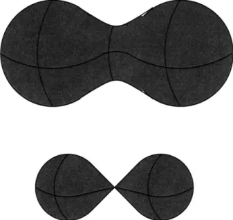
Figure 2-2: A surface in 3D that develops singularities and changes topology under mean curvature motion.
is that smooth closed curves in 2D shrink to a point under mean curvature motion [44, 46]. This theorem was proven in two steps. First, it was proved that smooth closed convex curves shrink to a point under this motion, becoming round in the limit. Second, it was proved that simple (not self-intersecting) closed planar curves become convex under this motion, thus completing the proof. For hypersurfaces of higher dimensionality, however, the behavior is not analogous. The usual counterexample is the case of a dumbbell-shaped surface in R3, as in Figure 2-2. Such a shape can easily be constructed so that it breaks into two pieces and develops singularities in finite time under mean curvature motion. That is, the evolution is smooth for a finite time period, but after that time period, cannot be continued in the same fashion.
One would like to continue the evolution even after the singularities develop. Presumably, the dumbbell should break into two separate pieces which should shrink smoothly. However, the representation of the shape directly as a parametrized surface cannot support this splitting. A more powerful representation is needed. The level set representation [88, 100] will be described in detail in this document as it is used in our system. The need for a representation that can handle topological changes and singularities is a major motivation for the level set methods. Similarly, the singularities that develop is one instance of the class of problems that motivated the development of viscosity solutions, which we will explain in section 2.3. The papers describing the level set method for mean curvature flow of arbitrary-dimensional hypersurfaces prove the correctness of the method for this problem "in a viscosity sense", which means, informally, that the solution is the smoothest approximation possible given the singularities present [38, 22].
We will see in section 3.4 that the image segmentation problem can be defined as minimizing a non-Euclidean curve length over all possible curves. The resulting curve flow equation obtained is closely related to 2.2. We will therefore be able to use much of the mathematical technology and results obtained for the mean curvature flow case for the image segmentation case. The definition of mean curvature is more complicated for manifolds that are not hypersurfaces. For completeness and because our studies have dealt with higher codimensional manifolds, we give this definition below.
2.1.2
Higher Codimension
For manifolds that are not hypersurfaces, there is not a single normal direction. Instead the dimensionality of the normal space is equal to the codimension of the manifold. Thus we no longer have a single well-defined normal direction. However, it turns out that one can compute the mean curvature normal vector uniquely as follows [102]. Let Mn = M C Rd be an n-dimensional manifold in Rd with codimension d-n.
Let M, and M' be the tangent and normal spaces, respectively, to M at point p. For any normal vector E Mg, we can define a mean curvature H in the direction of (. Like in the hypersurfaces case and as is intuitive, curvature measures the change in the tangent directions. Let X1, .. . , Xn be vector fields that are tangent to M that are
orthogonal to each other and unit length so that X1 (p),... Xn(p) is an orthonormal
basis for Mp. We then define the c-dependent mean curvature as
= Vxip)Xi
-where V' (p)Y is the covariant derivative of the vector field Y in the direction of
X (p).
It turns out that there is a unique vector 77(p) E M- such that
77(p)-= H for all E M'
and that this vector can be computed by summing the vectors obtained by multiply-ing each element of an orthonormal basis for M- by its direction-dependent mean
CHAPTER 2. BACKGROUND MATHEMATICS 17
curvature. Let vs 1,... ,vd be an orthonormal basis for M,', so
d n (p) = H,, vr r=n+1 1 d n
E!
(E
V, (P) Xi Vr) /r r=n+1 i=1 = rJ[ 'yXi, i=1where H denotes projection onto the normal space M.
As an example, let M be a 1D curve in R3. So the tangent space is 1-dimensional,
and X1 is the tangent field along M, and X1(p) is the tangent to M at point p. We
will choose the usual unit normal and unit binormal for a space curve as the basis vectors vi. These vectors are defined from the tangent t according to the first two
Frenet equations ([35])
t' = rN
N' = - - r B
where N is the unit normal, B is the unit binormal, K is the curvature of the curve, and r is its torsion. Further note that the covariant derivative of the tangent field in the direction of the tangent is the usual derivative t' of the tangent.
We then compute 3 1 n (P) =
Z(Z
V'(p)Xi - V,)Vr r=2 i=1 3 = Z(VX(pXl - V,)v, r=2 3 =: ZWt' Vr) Vr r=2 = (N -N)N + (nN - B)B = N + (O)B = N.Thus, we've shown that this definition for arbitrary dimensions does in fact reduce to the usual definition of the mean curvature vector for a curve.
The case of mean curvature flow for non-hypersurfaces has been less well-explored
hy-Figure 2-3: Under curve-shortening flow, the initial non-simple curve (solid) evolves into a curve (dashed) which contains a singularity.
persurfaces. The case of curve-shortening flow was studied for 3D curves [3] for the specific application of using this flow to address the limitation of planar curve flow that the curve be simple. When the initial curve is not simple then it can develop singularities after a finite time period, as pictured in Figure 2-3. In this example, the initial curve has a "figure eight" shape, and after evolving for some finite length of time, it develops a corner because the smaller circle in the figure eight shrinks to a point more slowly than does the larger circle. Altschuler and Grayson lifted the curves out of the plane by a small amount at the singular points and used the curve-shortening flow of space curves to implement the evolution of the original planar curve past these singularities.
It is the 3D version of curve-shortening flow which is most relevant to our CURVES system, as the objects to be segmented are modeled as 3D curves undergoing a motion related to curve-shortening flow. This curve flow is implemented in CURVES via level set methods, to which we now turn our attention.
2.2
Level Set Methods
Level set methods increase the dimensionality of the problem from the dimensionality
of the evolving manifold to the dimensionality of the embedding space [88, 100]. For the case of a planar curve, one defines a surface which implicitly encodes the curve, then evolves that surface instead of the explicit curve. An example of a surface as an implicit representation of a curve is the signed distance function pictured in Figure 2-4. In this case, let C be the curve, and the surface u is defined so that its value at any point is the signed distance to C, with interior points having negative distance by convention. C is then, by construction, the zero level set of u. The representations are equivalent in information content since one can generate the surface from the curve and the curve from the surface.
CHAPTER 2. BACKGROUND MATHEMATICS
U
u =1
C
U
=
0
Figure 2-4: Level sets of an embedding function u, for a closed curve in R2
.
2.2.1
Motivation
A brief discussion of the reasons why level set methods were developed is provided
be-fore a formal statement of the equivalence that underlies the methods. This discussion draws closely from [100], to which the reader is referred for further discussion.
Imagine we have some front C propagating over time. A necessary requirement for the use of the level set approach is that we care only about the front as a boundary between two regions. That is, we do not care about tangential motion of the front, but only about motion in the normal direction (Figure 2-5). As before, C is a function of both a spatial parameter and a time parameter, so we write C = C(p, t) where p E [0,1] is the spatial parameter and t > 0 is the time parameter.
We can write some equation for this motion as a partial differential equation: at each point on the curve C, the derivative of C with respect to time t is equal to a speed 3 times the normal N
Ct = ON, (2.3)
with initial condition C(., 0) = Co(-).
One problem with an explicit evolution of the curve is that singularities develop over time. This problem is a primary motivation for the use of level set methods. To understand this problem, first consider the case in which the initial curve can be written as a function of its spatial parameter. We will extend the intuition to functions that cannot be so written below; we discuss this case first because the derivatives are more natural.
The straightforward, explicit way to evolve the curve is to compute the normals analytically and use those normals to recompute the position of the curve at successive time steps. Consider the example of a cosine curve and assume we would like to propagate it forward in time with constant speed
#
= 1. This curve is plotted as thelowest curve in Figure 2-6(a). Successive curves are plotted above this curve of the evolution forward in time. The difficulty occurs at the convexity of the original curve.
Figure 2-5: A front propagating over time, where motion is assumed to be only in the direction of the normal vectors of the front.
A singularity develops eventually, after which time the normal is ambiguous. This
ambiguity implies that the evolution is no longer well-defined. Retaining all possible normal directions would cause the two "sides" of the front to intersect.
In order for the evolution to be well-defined, we need to choose one solution. The solution we choose is what is called the entropy solution, pictured in Figure
2-6(b). This solution is defined by the property that once a region has been crossed by the front, that region cannot be crossed again so the front cannot cross itself.
One often uses the analogy of a fire moving across a field, in which case the behavior is characterized by the statement, "Once a particle is burnt, it stays burnt." This statement is referred to as the entropy condition and the solution it implies as the
entropy solution because of the relation to information propagation. Information has
becomes lost when the singularity develops. Since the normal is not unique at that time and location, we cannot reverse the propagation to obtain the original curve.
We now make concrete the notion of "entropy solution". For the current cosine
example, if we change the speed 3 from 3 = 1 to 3 = 1 - er., for some small e and
where n is the Euclidean curvature of the front, then the singularities do not form. As
e approaches zero, the evolution approaches the entropy solution. Let Xatu,,e be
the evolution (the sequence of curves) obtained by using speed term
#
= 1 - ei. andXentn,p be the evolution obtained with the entropy condition. It can be proved that
the limit of the Xc,vature's as e approaches zero is identically the entropy solution:
Vt, limXrvature(t) = Xentro(t).
This limit, i.e. the entropy solution, is called the viscous limit and also the viscosity
solution of the given evolution. Viscosity solutions will be defined from a more formal
CHAPTER 2. BACKGROUND MATHEMATICS 21
Figure 2-6: Left image: the bottom curve is the initial cosine curve and the higher curves are successive curves obtained by propagating with normal speed 6 = 1. Right
image: continuing propagation after normal becomes ambiguous using entropy solu-tion.
its relevance to fluid dynamics. In fluid dynamics, any partial differential equation of the form
ut + [G(u)]x = 0
is known as a hyperbolic conservation law. A simple example is the motion of com-pressible fluid in one dimension, described by Burger's equation:
ut + UUX = 0.
To indicate viscosity of the fluid, one adds a diffusion (spatial second derivative) term to the right hand side to obtain
ut + uUX = EuXX
where e is the amount of viscosity. A well-known fact in the fluid dynamics community is that for e > 0, this motion remains smooth for all time: singularities, or shocks as
they are called in the fluid dynamics community, do not develop.
To relate the viscous limit to front propagation, we return to the idea of a curve propagating as in Figure 2-6. Let C = C(p) be the evolving front and Ct the change
in height of C in a unit time step. Referring to Figure 2-7, observe that the tangent at (p, C) is (1, C,) and notice that
Ct (I+ C2)1/2
wi 1
which gives the update rule
Ct
CP
B
Figure 2-7: Computation of motion Ct for relation of viscosity to front propagation. Setting the speed term to F = 1 - e, and observing that r, = CP/(1+
yields an equation which relates the motion Ct of the curve C to its spatial derivatives:
C- (1 + C,2)1/2 - CP
(1+ C2)
Differentiating with respect to p and setting u = to be the slope of the propa-gating front gives an evolution equation for u:
Ut + [-(1 + 2[1/2] =
U ~ (1 + U2)
Observe that this evolution equation is a hyperbolic conservation law. We observe that the curvature term in the speed function for a curve plays exactly the same role as the viscosity term in the evolution equation for the slope of the curve. It then follows that we can use the technology and theorems from fluid dynamics to prove that no singularities can develop in the slope of the front.
Sometimes we want to describe the motion of curves that are not expressible as functions. We thus cannot propagate them analytically. More importantly, we cannot detect singularities explicitly without the analytical form. Level set methods were developed to address exactly this issue. To summarize, they
" apply only to the situations in which we care about motion in the normal
direction but not in the tangential direction,
" address problems of singularities developing during an evolution, " evolve such fronts according to their entropy or viscosity solutions, and " are well-suited to boundaries which are not expressible as functions.
2.2.2
Hypersurfaces
We now explain the specific equivalence that underlies the level set methods. For the example of planar curves, let u : R2 -+
CHAPTER 2. BACKGROUND MATHEMATICS 23
Figure 2-8: Left: the initial value of the curve C is shown as a solid curve, and a later value is shown as a dashed curve. Right: The embedding surface u at the initial time (solid) and the later time (dashed).
C as in Figure 2-4, so C is the zero level-set of u. Let Co be the initial curve. It
is shown in [38, 22] that evolving C according to Equation 2.3 with initial condition
C(-, 0) = Co(-) for any function 0, is equivalent to evolving u according to
Ut = 0|vul (2.4)
with initial condition u(-, 0) = uo(-) and uo(Co) = 0 in the sense that the zero level set of u is identical to the evolving curve for all time. Referring to Figure 2-8 as an
example, if the solid initial curve in the left image evolved to the dashed curve, the
embedding surface would evolve as pictured in the right image.
Although this method may initially appear less efficient since the problem is now higher-dimensional, it has important advantages. First, it facilitates topolog-ical changes in the evolving manifold (the curve) over time. Evolving a curve directly
necessarily relies on a particular explicit parameterization of the curve, which makes
topological changes cumbersome, requiring special cases, whereas an implicit repre-sentation can handle them automatically as will be seen throughout this document. Parameterization is the heart of the second advantage of the implicit method as well: it is intrinsic (independent of parameterization). That is, it is an Eulerian
formula-tion of the problem which updates values at fixed grid points instead of a Lagrangian formulation which would move the points of the curve explicitly. The Eulerian
for-mulation is desirable for modeling curves in many applications including image seg-mentation since parameterizations are related only to the speed at which the curve is traversed, but not to its geometry. It is therefore problematic for a segmentation algorithm to depend on the curve's parameterization.
To see the equivalence geometrically, consider the zero level set
Differentiating with respect to t gives
Vu - Ft + Ut = 0
Further note that for any level set
Vu
=VU -N)
Ivul'
where N is the inward-pointing normal of the level set (for the case of a planar curve embedded in a surface, this level set is a curve). Substituting,
-NIVul
-P' + ut = 0.We want to define the evolution ut of u so that F C for all time; that is F(t) = C(t).
Having already initialized 1(0) = C(0), we only need set Ft = Ct to obtain
ut = #3Vul.
This derivation was given in [20], and is very similar to the derivation given in [87]. Moreover, it applies to hypersurfaces in any dimension [38, 22]; planar curves were used as an example for simplicity only.
It was shown that any embedding function u that is smooth in some open region of
RN and for some time period and whose spatial gradient does not vanish in that region
and time period is a viscosity solution to Equation 2.4 [38, 22]. Specifically, u must be Lipschitz continuous, where Lipschitz means that it cannot grow unboundedly: function f is Lipschitz if
If(x) - f(y) <; CIX - y1
for all x, y in the domain of
f
and for some constant C. It is also unnecessary to choose the zero level set of u: any isolevel set suffices, although the zero level set is the standard choice. For further detail, the reader is referred to [100], the primary reference for level set methods, implementation issues, and applications.One limitation of this body of work, as described until this point, is the restriction to hypersurfaces (manifolds of codimension one). The examples of a planar curve and a three-dimensional surface have codimension one, but space curves have codimension two. Intuition for why the level set method above no longer holds for space curves is that there is not an "inside" and an "outside" to a manifold with codimension larger than one, so one cannot create the embedding surface u in the same fashion as for planar curves; a distance function must be everywhere positive, and is thus singular on the curve itself. The more recent discovery of level set equations for curvature-based evolution in higher codimension [4], however, overcame this limitation.
CHAPTER 2. BACKGROUND MATHEMATICS
2.2.3
Higher Codimension
Ambrosio and Soner provided level set evolution equations for mean curvature flow of an arbitrary dimensional manifold in arbitrary dimensional space. Further, they gave the extension to more general curvature-based evolution which can incorporate an auxiliary externally defined vector field [4]. It is these equations that inspired our
CURVES segmentation algorithm which models blood vessels as curves in 3D, which
have codimension two. In particular, the auxiliary vector field equation enables the use of image information in addition to regularization. We now state these equations for the general case, as in [4].
Imagine we wish to represent and evolve some manifold F c Rd implicitly. Further assume that the codimension of F is k > 1. Let v : Rd -+ [0, oo) be an embedding
function whose zero level set is identically F, that is smooth near F, and such that Vv is non-zero outside F. For a nonzero vector q E Rd, define
Pq = I -I q|2
which is the projection operator onto the plane normal to q. Let X = PqAP for
some matrix A and let
A
1(X) A2(X) A_1(X)d...be the eigenvalues of X corresponding to the eigenvectors orthogonal to q. Notice that q will always be an eigenvector of X with eigenvalue 0.
Further define
d-k
F(q, A) = Ai(X).
i=1
Assuming the general case in which the only 0 eigenvalue corresponds to the eigen-vector orthogonal to q, we can say that F is the sum of the d - k smallest nonzero eigenvalues of X. It is then proved that the level set evolution equation to evolve F
by mean curvature flow is
Vt = F(Vv(x, t), V2v(x, t)).
(2.5)
That is, this evolution is equivalent to evolving F according to mean curvature flow in the sense that F is identical to the zero level set of v throughout the evolution.
For intuition, consider v as a distance function to F which thus satisfies
IVvI
= 1 everywhere except at F, although other functions are possible. Consider an isolevel set Fe ={xlv(x)
=4}
of v where e is very small and positive. Then the eigenvalues of 1X that are orthogonal to Vv are precisely the principal curvatures of theyVv hypersurface r,, oriented by Vv. Since IF has codimension k, we expect IF,, to havek - 1 very large principal curvatures and d - k principal curvatures related to the
geometry of F. For the lowest dimensional case in which F is a curve in R3, re is a thin tube around F, the larger principal curvature corresponds to the small radius of the tube, and the smaller principal curvature corresponds to the geometry of F. Note that the eigenvalues of 1 X are exactly the eigenvalues of x scaled by 1. Thus the use of X instead of 1X in Equation 2.5 is the same as using 1 X and scaling
by JVvj as in
d-k
V*) =|Ivv| Ai(i X).
i=1
|VV|
This alternate expression is perhaps more intuitive since the sum corresponds to curvatures so it looks like Equation 2.4.
Consider the situation in which there is an underlying vector field driving the evolution, in combination with the curvature term, so that the desired evolution equation is of the form
rt = r,] - Ed, (2.6)
where Ft gives the motion of the manifold F over time, , is the mean curvature of F,
I is the projection operator onto the normal space of F (which is a vector space of dimension d - k) and d is a given vector field in Rd. The evolution equation for the embedding space then becomes
Vt = F(Vv, V2v) + VV d.
(2.7)
2.2.4
Numerical Techniques
From the equations above, one does not yet have the full story about how to implement such evolutions. An underlying theme to both the direct curve evolution and the level-set based curve evolution is that we wish to compute temporal derivatives in terms of spatial derivatives. There is some discomfort in this notion since although the two are intimately related, it is not natural to regard one as a function of the other. In order to make this construction feasible, one must be careful about how exactly the spatial gradients are computed. Specifically, one should not use values at points that correspond to future times, in which the evolution has not yet occurred. That is, information should propagate in the same direction as the evolving front. Methods for gradient computation and for overall evolution are called upwind if they respect this restriction on information flow. That is, they use only values that are upwind of the direction of information propagation. This stability issue arises in the computation of the gradients needed in the update equation, Equation 2.4. Sethian discusses these issues in detail in his book [100]; we will provide intuition and then state the choices
CHAPTER 2. BACKGROUND MATHEMATICS
used for gradient computations.
A function f : R -+ R is said to be convex if its second derivative is everywhere
positive: f"(x) > 0. In higher dimensions, a function G : RN -+ R is convex if it is smooth and all second derivatives are everywhere non-negative: 92 ;> 0. One can also use an alternate definition that includes non-differentiable functions:
f
is convexif f (rx + (1 - T)y) <; f (x) + (1 - T)f(y), Vx, y E RN, 7T E [0, 1]. In the generalized
evolution equation
ut = H(x, u(x)U,u'(x)),
the term H(x, u(x), u'(x)) is called the Hamiltonian. In Equation 2.4, the Hamilto-nian is
#JVul
=/3
u,2 + u 2 + u,2, assuming 3 dimensions. We say that the speed function3
in an evolution equation is convex if the Hamiltonian/1Vul
is a convex function.Sethian provides numerical schemes for computation of gradients for both con-vex and non-concon-vex speed functions, and also for first order approximations to the gradient and for second order approximations to the gradient [100]. We review the first-order convex case here for discussion purposes. First, some notations:
The central difference operator, forward difference operator, and backward
dif-ference operator for first-order approximating the spatial derivative of u in the x
dimension, at grid point (i, j, k), are, respectively, DFXk = Dik = _ Ui+l,j,k - Ui-,j,k
23k 2Ax
-t Dtxu -Ui±1,,k 2Ax- Ui,3,k
Dt- = Dxu = Uij,k - Ui,j,k
Taylor series expansions around x show that
ux=DFkO 2)
u=Dilk + 0(h2
ux Dtkx + O(h)
UX Dk + O(h),
where h is the spacing between adjacent grid points. We thus see that the central difference scheme yields the most accurate approximation. However, when handling moving fronts, the issue of direction of information propagation is also important, so we will see that it is suboptimal in some cases.
First Order, Space Convex
An example of a convex speed function is a constant speed function applied to an embedding space u which has constant slope. Let F be any convex speed function, and assume we have the evolution equation
ut + FIVu|= 0.
The first order upwind scheme for iteratively solving this equation ([100, 88]) is then
uij =iu - At[max(Fijk, O)V+ + min(Fijk, 0)V-, (2.8)
where V+= [max(D-', 0)2 + min(D-t, 0)2 + max(Di, 0)2 + min(Dj, 0)2 + max(D-', 0)2 + min(D+I, 0)2 + and V = [max(Dt', 0)2 + min(Dj, 0)2 + max(D+I, 0)2 + min(D-1, 0)2 + max(Dtk, 0)2 + min(Dej, 0)2].
To demonstrate the importance of choosing the correct scheme for gradient com-putation, we constructed a simple experiment in which a front is propagating outward at constant speed F = 1. Assuming u is a distance function so IVul = 1 everywhere,
this speed function is convex because FiVul is constant so all of its second derivatives are 0. In this case, we have
ut +l1Vul =0,
and Equation 2.8 becomes
i= Uk - At[V+] (2.9)
ijk - At[max(Dj', 0)2 + min(Dt', 0)2 + (2.10)
max(Dj, 0)2 + min(D+Y, 0)2 + (2.11) max(Dg, 0)2 + min(Dt, 0)2]i. (2.12) Imagine that each slice of our embedding surface is identical at time t = 0, and
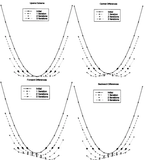
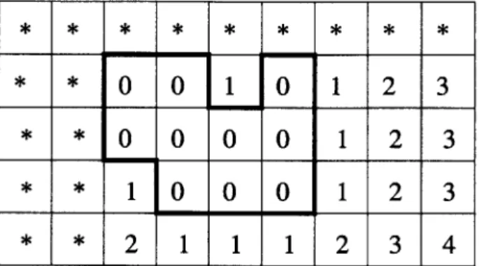
CHAPTER 2. BACKGROUND MATHEMATICS Upwirid SchMe -.-- Initial 1-4 iherafion 24 2teraion 3-4- 3lteralon /X\ A / \ X 'A.I I 'k k /trto 2 / \aon 3! .4rac -K I 2ltarations 24 -3teration * , 0 X . I /X InK/ I Itrto / ' / I 2 Itrbn 34 .4te/ '3
Figure 2-9: Cross-sectional slices for a front moving with constant unit speed. Behav-ior is shown for four different numerical methods of gradient approximation: upper left is upwind scheme, upper right is central difference scheme, lower left is forward difference scheme, and lower right is backward difference scheme.
straight lines in the direction normal to the figures, and the outward direction is the direction towards the edges of the plots. What Figure 2-9 shows is the evolution computed, for At = 1 and three iterations, for four difference methods of finite
gradient approximation. The upper left plot shows the upwind scheme, the upper right the central difference scheme DF-k, the lower left the forward difference scheme
D", and the lower right the backward difference scheme. Points on the zero level
set which correspond to the contour itself moving over time are marked in black. For this particular example,
IVul
is one everywhere initially. This implies that any one-sided difference scheme will work: the backward and forward schemes thus give the desired evolution, as does the upwind scheme away from the singularities. The upwind scheme differs from the desired behavior at exactly the singularities because it is at those points that it chooses either both or neither of the difference operators,Upwind Scheme Initial - -- 1 Iteration 2 Iterations - 3 Iterations / X Forward Differences --a 1iteraion a' 2 Iteratios -- 34 tembtona Nt a 14 YA a I a / 41 7A' Wc , Central Diffrences - -- InItial I teration a' 2 Iterations -- 3- Sterations IIt Itnraa a X IItrto .4 2 te1d -X_ teraions IC 2 Itration -.-- 3tealn X1 ib.
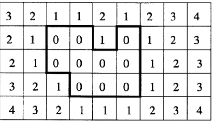
Figure 2-10: Cross-sectional slices for another front moving with constant unit speed. Upper left is upwind scheme, upper right is central difference scheme, lower left is forward difference scheme, and lower right is backward difference scheme.
so is not using exactly one of them and is thus not obtaining a slope of one. Notice that the central difference scheme, although theoretically more accurate than the one-sided schemes, gives worse behavior. It develops a local maximum at the center point of the plot, and has developed multiple undesirable local maxima by the third iteration.
Figure 2-9 shows an example in which any one-sided scheme is effective. When
IVul
: 1, however, one cannot simply use any one-sided scheme. In general, evenif one initializes the evolution with an embedding function u such that
IVul
= 1everywhere, the evolution will not maintain this invariant over time with a non-constant speed function. Hence, one should not use simple forward or backward differencing in general. Figure 2-10 demonstrates a case in which the initial embedding
CHAPTER 2. BACKGROUND MATHEMATICS
surface u is parabolic, so does not have slope one. In this case, we are still using constant speed F = 1. Note that we still have a convex speed function because the
second derivatives are constant for a parabolic u and constant F. Observe that the forward and backward differencing schemes yield different behaviors, with the zero-level-set points becoming spaced unequally on the opposite sides of the center. This is clearly wrong. The central differencing scheme naturally maintains symmetry, but develops an undesirable singularity at the original center point. The upwind scheme is most effective here.
Hybrid Speed Functions
Imagine a speed function F is the sum of multiple speed functions each of which would require different schemes for computation of Vu. In this case, Sethian advises to use the correct, and different, gradient computations for each term [100]. The example of a speed function which is a sum of a curvature term and a term related to an external vector field is important for the application of image segmentation, as we will see in Chapter 3.4, so we will describe that case here. This is a subpart of an example provided in [100]. Assume
F = Fcurv + Fext,
where Fu,-v = -En is the curvature-related component of the speed with e a small
positive constant and , the curvature of the front, Fext = E(x, y) -n' is the component
that depends on an external vector field, with n the unit normal to the front. The equation for the embedding space u is then
Ut = eKIVuI - E(x, y) -Vu.
The curvature term is based on second derivatives so uses information from both sides of the front; that is, information propagates in both directions. Thus, Sethian advocates the uses of central differences for the curvature term. The other term corresponds to a speed independent of u, so one should use an upwind scheme just as in the previous example of F = 1. The numerical update rule for u becomes
+[EK-(D 2+ DY
2-[max(fij, 0)D-x + min(fi3, 0)D-x
. +max(gij, 0)D-Y + min(gi, 0)Dy]_
where E = (f, g) and K is the approximation to the curvature computed using
second differences on the level set (Equation 5.10).