Continuous low-rank tensor decompositions, with
applications to stochastic optimal control and data
assimilation
by
Alex Arkady Gorodetsky
B.S.E., University of Michigan (2010)
S.M., Massachusetts Institute of Technology (2012)
Submitted to the Department of Aeronautics and Astronautics
in partial fulfillment of the requirements for the degree of
Doctor of Philosophy in Computational Science and Engineering
at the
MASSACHUSETTS INSTITUTE OF TECHNOLOGY
February 2017
@
Massachusetts Institute of Technology 2017.
Author ... Certified by. Certified by... Certified by.. Accepted by.. Accepted by..
All rights reserved.
Signature redacted
Department of Aeronautics and Astronautics
Signature redacted
September 2, 2016... Sertac Karaman Associate Professor, Aeronautics and Astronautics
Signature redacted-
... Thesis Supervisor... . ... Youssef M. Marzouk Associate Professor, Aeronautics and Astronauticsa Thesis Supervisor
Pierre Lermusiaux Associate Professor, Mechanical Engineering
Signature redacted
Theis
CommitteE
MASSA098_%TTS INSTITUTE OF TECHNOLOGY
MAR 09 201
Youssef M. Marzouk Associate Professor, Aeronautics and Astronautics Co-Directo , Computational Science and Engineering
Signature redacted
Youssef M. Marzouk Associate Professor, Aeronautics and Astronautics Chair, Graduate Program Committee
Continuous low-rank tensor decompositions, with applications
to stochastic optimal control and data assimilation
by
Alex Arkady Gorodetsky
Submitted to the Department of Aeronautics and Astronautics on September 2, 2016, in partial fulfillment of the
requirements for the degree of
Doctor of Philosophy in Computational Science and Engineering
Abstract
Optimal decision making under uncertainty is critical for control and optimization of complex systems. However, many techniques for solving problems such as stochastic optimal control and data assimilation encounter the curse of dimensionality when too many state variables are involved. In this thesis, we propose a framework for computing with high-dimensional functions that mitigates this exponential growth in complexity for problems with separable structure.
Our framework tightly integrates two emerging areas: tensor decompositions and continuous computation. Tensor decompositions are able to effectively compress and operate with low-rank multidimensional arrays. Continuous computation is a paradigm for computing with functions instead of arrays, and it is best realized by Chebfun, a MATLAB package for computing with functions of up to three dimen-sions. Continuous computation provides a natural framework for building numerical algorithms that effectively, naturally, and automatically adapt to problem structure. The first part of this thesis describes a compressed continuous computation frame-work centered around a continuous analogue to the (discrete) tensor-train decompo-sition called the function-train decompodecompo-sition. Computation with the function-train requires continuous matrix factorizations and continuous numerical linear algebra. Continuous analogues are presented for performing cross approximation; rounding; multilinear algebra operations such as addition, multiplication, integration, and dif-ferentiation; and continuous, rank-revealing, alternating least squares.
Advantages of the function-train over the tensor-train include the ability to
adap-tively approximate functions and the ability to compute with functions that are
pa-rameterized differently. For example, while elementwise multiplication between ten-sors of different sizes is undefined, functions in FT format can be readily multiplied together.
Next, we develop compressed versions of value iteration, policy iteration, and multilevel algorithms for solving dynamic programming problems arising in stochastic optimal control. These techniques enable computing global solutions to a broader set of problems, for example those with non-affine control inputs, than previously
possible. Examples are presented for motion planning with robotic systems that have up to seven states. Finally, we use the FT to extend integration-based Gaussian filtering to larger state spaces than previously considered. Examples are presented for dynamical systems with up to twenty states.
Thesis Supervisor: Sertac Karaman
Title: Associate Professor, Aeronautics and Astronautics
Thesis Supervisor: Youssef M. Marzouk
Title: Associate Professor, Aeronautics and Astronautics
Committee Member: Pierre Lermusiaux
Acknowledgments
This work would not have been possible without the support of so many people. First, I thank my advisors, Youssef Marzouk and Sertac Karaman. Over the last six years, Youssef has provided me valuable guidance and the freedom to pursue my ideas and academic interests. I also thank him for giving me the opportunity to travel to conferences and do summer internships. They were invaluable experiences. I thank Sertac for introducing me to a new field and providing me the opportunity to really push and extend my research. His encouragement and excitement enabled me to persevere. I also thank Professor Pierre Lermusiaux, Dr. Tamara Kolda, and Professor John Tsitsiklis for providing valuable feedback on my thesis.
ACDL has been a fantastic place to grow up as a researcher. It was a great source of feedback and ideas. In particular, I am indebted to Tarek Moselhy, Chad Lieberman, Doug Allaire, Alessio Spantini, and Daniele Bigoni for the remarkable help they have given me over the last years.
I also thank Fabian Riether for making my code fly, and John Alora, Chris Grimm, and Ezra Tal for their great and rewarding collaborations.
Finally, I thank my family for their support and encouragement. They gave me motivation to continue and provided meaning to my work.
Contents
1 Introduction 15
1.1 Motivation: decision making under uncertainty . . . . 16
1.2 Computing with functions . . . . 19
1.3 Objectives and contributions . . . . 23
1.4 Thesis outline . . . . 24
2 Continuous linear algebra 25 2.1 Scalar-, vector-, and matrix-valued functions . . . . 26
2.1.1 Definitions and interpretations . . . . 27
2.1.2 M ultiplication . . . . 32
2.2 Continuous matrix factorizations . . . . 33
2.3 Skeleton decomposition and cross approximation . . . . 37
2.3.1 Existence of the skeleton decomposition of vector-valued functions 40 2.3.2 Optimality of maxvol . . . . 45
2.3.3 Cross approximation and maxvol . . . . 46
2.4 Operations with functions expressed in an orthonormal basis . . . . . 52
2.4.1 Scalar-valued functions . . . . 52
2.4.2 Vector-valued functions . . . . 54
2.4.3 Matrix-valued functions . . . . 55
3 Function-train decomposition 61 3.1 Discrete tensor decompositions . . . . 62
3.2.1 3.2.2
FT for functions with finite-rank unfoldings . . . . FT for functions with approximately low-rank unfoldings 3.3 Continuous cross approximation and rounding . . . .
3.3.1 Cross approximation of multivariate functions 3.3.2 Rounding and rank adaptation . . . . 3.4 Continuous multilinear algebra . . . . 3.5 Continuous rank-revealing alternating least squares . 3.5.1 Optimization algorithm . . . . 3.5.2 Example: multiplication . . . . 3.5.3 Example: diffusion operator . . . . 3.6 Numerical examples . . . . 3.6.1 Implementation details . . . . 3.6.2 Integration . . . . 3.6.3 Approximation . . . . 3.7 Summary . . . .
4 Low-rank algorithms for stochastic optimal control
4.1 Continuous-time and continuous-space stochastic optimal control . 4.1.1 Stochastic differential equations . . . . 4.1.2 Cost functions . . . . 4.1.3 Markovian policies . . . . 4.1.4 Dynamic programming . . . . 4.2 Discretization-based solution algorithms . . . . 4.2.1 Discrete-time and discrete-space Markov decision processes 4.2.2 Markov chain approximation method . . . . 4.2.3 Value iteration, policy iteration, and multilevel methods . 4.3 Low-rank dynamic programming algorithms . . . . 4.3.1 FT representation of value functions . . . . 4.3.2 FT-based value iteration . . . . 4.3.3 FT-based policy iteration . . . .
. 69 . 69 . . . . 70 . . . . 71 . . . . 73 . . . . 78 . . . . 81 . . . . 83 . . . . 89 . . . . 90 . . . . 95 . . . . 96 . . . . 101 . . . . 104 . . . . 110 113 114 114 115 117 118 119 120 121 128 134 135 137 138
4.3.4 FT-based prolongation and interpolation operators . . . . 139
4.4 A nalysis . . . . 141
4.4.1 Convergence of approximate fixed-point iterations . . . . 142
4.4.2 Convergence of FT-based fixed-point iterations . . . . 146
4.4.3 Complexity of FT-based DP algorithms . . . . 148
4.5 Numerical examples . . . . 149
4.5.1 Linear-Quadratic-Gaussian with bounded controls . . . . 150
4.5.2 Car dynamics . . . . 157
4.5.3 Perching glider dynamics . . . . 162
4.5.4 Quadcopter dynamics . . . . 166
5 Low-rank algorithms for Gaussian filtering 171 5.1 Filtering problem . . . . 172
5.1.1 Continuous time state evolution . . . . 172
5.1.2 Existing algorithmic frameworks . . . . 174
5.1.3 Integration based Gaussian filtering equations . . . . 176
5.2 Low-rank filtering algorithms . . . . 179
5.2.1 Low-rank tensor product quadrature . . . . 180
5.2.2 FT-based integration filter . . . . 181
5.3 Numerical examples. . . . . 182
6 Conclusion 189 6.1 Sum m ary . . . . 189
6.2 Future w ork . . . . 191
A Additional lemmas and proofs 193 A.1 Proof of Theorem 2 . . . . 193
A.2 Eigenvalues of a discretized kernel . . . . 195
A.3 Proof of Theorem 3 . . . . 196
A.4 Proof of Theorem 4 . . . . 198
List of Figures
1-1 Discretized vs. parameterized functions. . . . . 21
2-1 Vector and matrix interpretations of scalar-valued functions . . . . . 28
2-2 Vector-valued functions as vectors and matrices in continuous linear algebra . . . . 29
2-3 Visualization of unfoldings Fk of a vector-valued function F . . . . . 30
2-4 Visualization of a matrix-valued function F. . . . . 31
2-5 Fibers of a vector-valued function in k-separated form . . . . 38
3-1 Scaling of continuous ALS for multiplication. . . . . 90
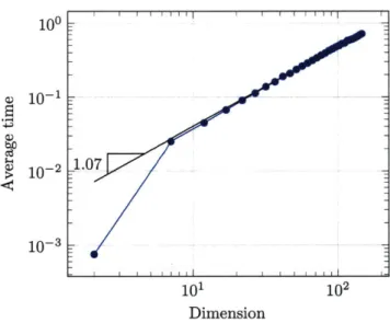
3-2 Linear scaling of continuous ALS with dimension for diffusion. ... 94
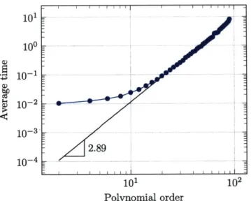
3-3 Cubic scaling of continuous ALS with polynomial expansion order for diffusion . . . . 95
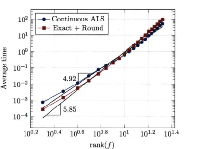
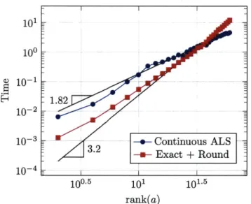
3-4 Scaling of continuous ALS with respect to the rank of the conductivity field . . . . 96
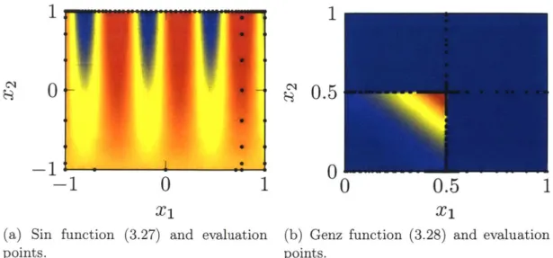
3-5 Contour plots and evaluations of fi and f2. . . . . 100
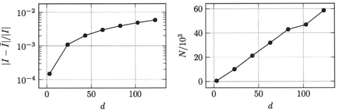
3-6 Error and computational complexity for integrating a periodic Genz function . . . . 102
3-7 Error and computational complexity for integrating a discontinuous G enz function . . . . 103
3-8 Performance of rank-adaptive cross approximation on an elliptic PDE. 109 4-1 An illustration of a continuous-time interpolation of a discrete process arising from the Markov chain approximation. . . . . 122
4-2 Sample discretization of a two-dimensional state space. . . . . 125 4-3 Cost functions for the LQG problem with different control bounds and
absorbing boundaries . . . . 151 4-4 Cost functions and ranks for the LQG problem with different diffusion
magnitudes and absorbing boundaries. . . . . 153 4-5 Cost functions for the LQG problem with different control bounds and
reflecting boundaries. . . . 154 4-6 Cost functions and ranks for the LQG problem with different diffusion
magnitudes and reflecting boundaries . . . 156 4-7 FT-based value iteration diagnostic plots for the LQG problem with
reflecting boundaries . . . 157 4-8 FT-based policy iteration diagnostic plots for the LQG problem with
reflecting boundaries . . . 158 4-9 Trajectories of the Dubin's car for three initial conditions. . . . . 159 4-10 One-way multigrid for solving the Dubin's car control problem. . . . . 160 4-11 Trajectories of the understeered car for three initial conditions. . . . . 161 4-12 One-way multigrid for solving the understeered car control problem. . 162 4-13 Trajectories of the perching glider for three initial conditions. . . . 164 4-14 One-way multigrid for solving the perching glider control problem. . . 165 4-15 Trajectories of the quadcopter for three initial conditions. . . . . 168 4-16 Three-dimensional trajectories showing the position of the quadcopter
for various initial conditions. . . . 169 4-17 One-way multigrid for solving the quadcopter control problem. . . . . 169
5-1 Comparison of computational time and variance obtained between fully tensorized Gauss-Hermite filter (GHF) and the low-rank tensor-train GHF (TTGHF). . . . . 184 5-2 Filtering of the Lorenz 63 system. . . . . 185 5-3 Filtering of the Lorenz 96 system. . . . . 186
List of Tables
2.1 Products between vector
/matrix-valued
functions and vectors/matrices.
32 2.2 Product of two vector-valued functions (top left); a vector-valuedtion and a matrix-valued function (bottom left); a matrix-valued tion and a vector-valued function (top right); two matrix-valued func-tions (bottom right). . . . . 32
3.1 Algorithmic parameters used for approximation of the simulation li-brary benchmark problems. . . . . 104 3.2 Performance of the FT approximation algorithm on a set of
multi-dimensional test functions from the Simulation Library Test Func-tions [113]. . . . . 106
Chapter 1
Introduction
Numerical methods and algorithms that enable computational modeling are impor-tant drivers of advancement in science and engineering. They help increase the scope and capabilities of computational models that, in turn, have dramatic impacts on so-ciety. For example, computational modeling has played a primary role in discovering unseen planets in our solar system
[5],
has assisted in the creation of autonomous systems that are able to identify new biological mechanisms [111], and has led to novel airplane designs that are largely designed, tested, and verified using computa-tional techniques [114]. Society also depends heavily on computacomputa-tional modeling for a diverse set of needs such as weather prediction, financial market management, evalu-ation of economic policies, medical data analysis, and more. All of these systems rely on fast, effective, and accurate numerical algorithms that underpin computational models.The utility of computational modeling and simulation for design, analysis, and control has resulted in an ever growing desire to increase the complexity of modeled systems. As computational scientists continue to try to model real systems with increasing levels of reality, they begin to use more detailed equations and larger amounts of data. The resulting increase in model complexity causes trouble for many existing numerical algorithms.
In this thesis, numerical techniques are developed that strive to enable compu-tation for the increasingly complex models that are encountered in practice. The
techniques are the result of an integration of two areas: tensor decompositions and function approximation. Tensor decompositions have been shown to mitigate the curse of dimensionality associated with storing large amounts of discrete data. Func-tion approximaFunc-tion has become extremely effective for developing accurate simplifica-tions of complex models to aid in their analysis. Integrating these two areas produces a framework that automatically adapts to problem structure, provides an efficient rep-resentation for computation, and mitigates the curse of dimensionality in a variety of application areas. Applications of the resulting techniques are shown for stochastic optimal control and data assimilation.
1.1
Motivation: decision making under uncertainty
This research is motivated to create computational algorithms that perform auto-mated decision making under uncertainty. Arguably, decision making under uncer-tainty is one of the biggest factors motivating the development of computational science. Optimal decision making in the presence of real-world uncertainties can potentially revolutionize countless scientific, engineering, and societal endeavors. Al-gorithmic breakthroughs in this area have potential for being the enabling technology for autonomous robotic systems that can effectively explore and monitor dangerous environments on and off Earth. They can enable efficient resource allocation and ro-bust performance of national infrastructure such as the energy grid and transportation networks. Finally, optimal automated decision making under uncertainty will become a critical tool for analyzing and regulating complex systems such as social networks; applications can include resource allocation for preventing the spread of contagious diseases and optimal sensor placements for safety monitoring of water networks.
Automated decision making under uncertainty, however, remains a challenging task that is plagued by the curse of dimensionality: its computational expense grows exponentially with the number of degrees of freedom. Indeed, all aspects of decision making under uncertainty including data analysis
[39],
Bayesian inference and un-certainty quantification [10, 34], and Markov decision processes (MDP) [102,105] areafflicted.
Richard Bellman, whose namesake is the well known Bellman equation, defined the term curse of dimensionality [8] in the context of optimization methods. He provides the following example about the difficulty of optimization by enumeration in tensor product spaces: if each dimension is discretized into 10 points, then a ten-dimensional problem would have a search space of 1010 points, a twenty-ten-dimensional problem would have a search space of 1020, and a hundred-dimensional problem would have a search space of 10100 dimensions - more than the number of estimated atoms
in the universe (1078 - 1082)!
The Bellman equation describes the solution of a dynamic programming (DP) problem. Mitigating the curse of dimensionality associated with DP would greatly enhance the capabilities of automated decision making under uncertainty since DP is a general and versatile framework for formulating decision problems [12,13,15,102]. For example, stochastic shortest path [14] problems, stochastic optimal control problems, and more generally, Markov decision processes can be formulated as dynamic pro-gramming problems. Parallel computing methods can sometimes reduce the compu-tational time for finding its solution, but some results suggest that stochastic Markov decision processes are inherently sequential and may not benefit too greatly from parallelization [99]. Thus, fundamentally new algorithms are needed to enable so-lutions for DP for a wider variety of systems. The algorithms that we propose in Chapter 4 are indeed sequential,f but they exploit a particular type of problem struc-ture that enables computational feasibility. Other areas related to MDPs also suffer in high dimensions. For example, partially observable Markov decision processes (POMDPs) [20,25,85,115], which can be formulated as an MDP with states that are probability distributions, are notoriously difficult to solve.
Beyond optimization, Donoho points out that this problem also exists in function approximation and numerical integration [39]. He notes that to approximate a func-tion of d variables, when it is only known that the funcfunc-tion is Lipschitz, requires on the order of (1/E)d evaluations on a grid to obtain a uniform approximation error of
(1/E)d for an integration scheme to have an error of c.
Despite these incredible demands, effective numerical optimization, function ap-proximation, and numerical integration are vital to the pursuit of computational algorithms for decision making under uncertainty. Many uncertainty quantification methods such as uncertainty propagation and Bayesian inference can be argued to be exercises in integration. Consider that extracting information from probability distributions requires the evaluation of integrals. In order to be able to solve these problems effectively, numerical methods that exploit more problem structure than just Lipschitz continuity must be developed.
The Monte Carlo method is one example of a ubiquitous algorithm within un-certainty quantification and optimization that is relied upon to mitigate the curse of dimensionality. However, many Monte Carlo algorithms themselves run into the curse of dimensionality. For example, the particle filtering algorithm for data assimilation attempts to propagate a distribution represented by samples through a dynamical system and through Bayes' rule. Particle filtering notoriously runs into problems due to sample impoverishment [10, 34], and an exponentially growing number of samples are needed as the dimension of the system increases [110].
Furthermore, the standard Monte Carlo estimator (without particle filtering) can also run into the curse of dimensionality since the variance of the estimator is pro-portional to the variance of the random variable whose mean is being estimated. Consider the simple function fd(X1, . .., Xd) = X, .. Xd where Xi are independent
and identically distributed random variables with mean 0 and variance 2. In this case we have
var(fd) = E [(X1 ... Xd) 2] - (E [X1 ... Xd])2 =E [X2 --- X2] - (E [X1]) 2 ...-(E [Xd])2
E1
[X2]
... E
[X2]
_-1 XI2.. E[dd d
=
]
(var(Xi) + (E [Xi]) 2) -- (E [Xi])2,which for our case means
var(fd) = 2
Therefore, the number of samples required to estimate the expectation of fd grows
exponentially with dimension to achieve similar levels of accuracy. Practitioners typ-ically hope that the variance of their outputs does not grow exponentially with the complexity of their models, so that the number of required samples (and therefore the computational cost of analysis) does not grow exponentially.
We are motivated to seek other methods that can mitigate the curse of dimension-ality to develop algorithms that converge faster than the AfNf rate associated with Monte Carlo. While Monte Carlo requires that the variance of our models does not grow too fast, the primary type of structure exploited in this research is that of output
separability. The separability of a function refers to the notion that a multivariate
function can be approximated by the sum of the products of univariate functions, e.g.,
R
f (X1, . .. , Xd) = 1 # (XI) . .. O (Xd).
i=1
If the rank R is "small", then
f
is considered to be a low-rank function. Low-rank functions can be integrated with complexity that is linear in dimension and polynomial with the rank. For example, the function fd described above is rank 1, and it canbe integrated with a computational cost that scales linearly with dimension. We hypothesize that separable structure is prevalent in many relevant application areas, and we show that its exploitation is indeed feasible for certain stochastic optimal control and data assimilation problems. The resulting methods can be viewed as complementary tools to Monte Carlo methods for high dimensional problems.
1.2
Computing with functions
One of the main ways to combat the computationally intensive nature of algorithms in high dimensions is through approximating the computationally expensive aspects of the problem in a simpler way. For example, one expensive aspect of Markov chain
Monte Carlo, a Monte Carlo variant that is useful for sampling from arbitrary dis-tributions, is repeated evaluations of the likelihood function. These evaluations are
particularly expensive when they involve solutions to partial differential equations (PDEs). A common strategy in these situations is to replace the likelihood with a surrogate model or emulator [31,88]. Then, instead of evaluating a PDE, the surrogate model is used within the evaluation of the likelihood. Surrogate models also play a role in solving Markov decision processes. Approximate dynamic programming [15,102] often use surrogate modeling techniques to transform a computationally infeasible problem to a simpler one by using a finite dimensional representation for the
ap-proximation of a value function. In general, function apap-proximation techniques for
generating surrogate models play an important role in a wide variety of numerical algorithms.
This thesis is partially inspired by the pioneering view on the use of function ap-proximation within computation developed by Trefethen, Battles, Platte, Townsend,
and others, that is realized through the Chebfun package for the MATLAB computer
language [4,101,117-119]. Their view is that end users of numerical software are typically interested in computing with functions instead of arrays. Users often have
PDEs, optimization problems, or inference problems that are defined in continuous
spaces in terms of functions. Extracting information from these functions,
represent-ing them on the computer, and performrepresent-ing operations with them should be within the domain of the software, not the user. The user should not have to specify that
they would like to discretize their functions using a particular grid or represent them with a particular parameterization. Instead, the user should only need to specify the
accuracy with which they want to compute or a storage level they would like to stay
within.
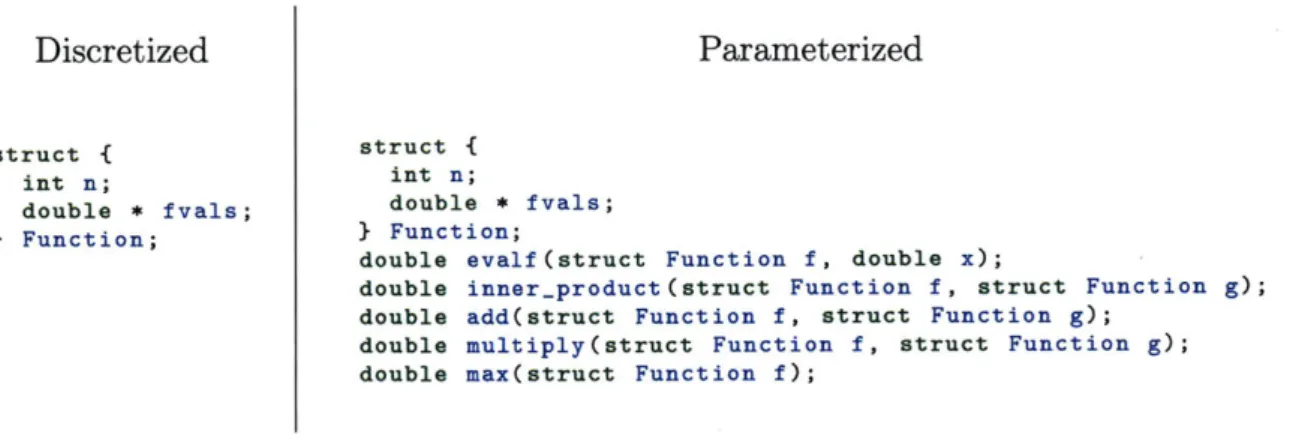
The fundamental backbone that allows for such a beautiful possibility lies in in-terpreting continuous objects on a computer not as being discretized but rather
pa-rameterized. We purposely make a subtle, but vitally important, distinction between
discretization and parameterization. For us, discretization implies that the computer
Pa-Parameterized
struct { struct {
int n; int n;
double * fvals; double * fvals;
} Function; } Function;
double evalf(struct Function f, double x);
double innerproduct(struct Function f, struct Function g); double add(struct Function f, struct Function g);
double multiply(struct Function f, struct Function g); double max(struct Function f);
Figure 1-1: Discretized vs. parameterized functions.
rameterization implies that the computer can "see" a function on a computer through a finite set of parameters and a set of routines that map those parameters to outputs of interest.
As an example, consider a function discretized onto some grid of n points that
results in the function values {fl, . .. ,
fn'}.
A discretization viewpoint might storethis function as an array of floating point values.
fl f2 .. . ffn
The continuous framework utilizing the parameterized viewpoint, on the other hand, would store this function as an object that contains the function values and various routines for evaluating the function at arbitrary locations, computing inner prod-ucts, finding its maximum, etc. These routines would be created by interpreting the discretized function values as, for instance, nodes of a spline or linear element approx-imation. The encoding for the discretized and the parameterized functions in the C programming language would then look similar to Figure 1-1.
The resulting effect on numerical algorithms is tremendous. Consider a matrix whose columns consists of m different functions. Performing matrix-factorization such as the QR or LU decompositions now takes on a new meaning. In the discretized framework, the m functions are each evaluated at n locations and the standard ma-trix QR and LU decompositions are performed. In the parameterized format the
m functions may still be evaluated at n locations, but the QR and LU
tions are modified because the inner product is a continuous inner product in the
QR
decomposition and the pivots for the LU are chosen using a continuous max-imization technique. Put another way, in the discretized framework linear algebra algorithms can only work with discrete inner products, discrete maximization, ele-mentwise addition, eleele-mentwise multiplication, etc. These discrete algorithms use no other information about the function that is actually being represented.There are both theoretical and practical advantages to using this continuous frame-work. Theoretically, one can begin to link the convergence of matrix factorizations such as the QR, LU, and SVD decompositions to properties of the original func-tions [118]. The practical advantages include automated adaptation and better error control for operations with functions. For example, if an algorithm calls for multi-plying two functions together, the resulting function often needs to be parameterized by a larger set of parameters to maintain accuracy. Instead, if functions are simply multiplied using elementwise multiplication of their discretizations, then the resulting product may not accurately represent the continuous product between the original functions. Furthermore, performing multiplication, addition, and taking the inner product between functions that are discretized in different ways is ill-defined. Such operations would effectively force the user to provide the computer with more infor-mation.
While continuous computation has been effectively developed for univariate and bivariate functions by the Chebfun package, theory and routines for representing and operating with general multivariate functions has up to now been lacking. The major goal in this thesis is to develop a framework for continuous computation for high-dimensional functions. One realization of this framework is the new numerical computing software package Compressed Continuous Computation (C3) [54] that is
used for most of the numerical examples within this thesis.
The new framework relies on representing functions in a compressed format that is a continuous extension of low-rank tensor decompositions. In contrast to other low-rank functional approaches [26,40, 103], however, our framework provides more flexibility and generality. The previous approaches all rely on converting a low-rank
functional approximation problem to a low-rank tensor approximation problem, where the tensor represents certain parameters of the function approximation scheme that are linearly related to the output. Our framework never requires this conversion, in fact, the resulting algorithms for high-dimensional computation are independent from the underlying parameterization. In the end, our ability to incorporate a wider variety of, even nonlinear, parameterizations results in a more general framework than these previous approaches.
1.3
Objectives and contributions
The primary objective of this research is to develop a framework for continuous com-putation with multivariate functions. Two secondary objectives are to develop scal-able algorithms for (1) stochastic optimal control and (2) data assimilation. The solution to the primary objective enables the design of novel algorithms for tackling the secondary objectives. The major high-level contributions of this research are then
1. A framework for continuous computation with multivariate functions that ex-ploits low-rank tensor decompositions,
2. Application of a low-rank framework for the solution of dynamic programming equations arising in stochastic optimal control, and
3. Application of continuous computation to integration-based Gaussian filtering.
Numerous lower-level contributions were necessary for the realization of these objectives. For the development of continuous computation, we make the following contributions:
e Development of maximum-volume based CUR/skeleton decompositions of vector-valued functions,
e Extension of continuous matrix factorizations to the case of QR and LU factor-ization of matrix-valued functions, and
* Continuous versions of cross approximation, rounding, and alternating least squares for a continuous tensor-train decomposition - called the function-train (FT) decomposition.
For the application of the low-rank framework to stochastic optimal control and data assimilation, we make the following contributions:
" Utilization of the function-train decomposition within value and policy iteration for solving Bellman's equation,
" Utilization of the function-train decomposition for multi-level schemes by en-abling evaluations of optimal value functions and policies in continuous domains, and
* Utilization of the function-train for multivariate integration within integration-based Gaussian filtering.
1.4
Thesis outline
The thesis is organized as follows. In Chapter 2, the continuous linear algebra back-ground is provided. In that chapter, all of the continuous linear algebra that is used throughout this thesis is described and discussed. Chapter 3 describes the novel low-rank functional decomposition, the function-train (FT). The FT is shown to be the continuous analogue of the discrete tensor-train decomposition. All the continuous analogues of operations performed with the discrete tensor-train are then described. These operations include cross approximation, rounding, multilinear algebra, and al-ternating least squares. Chapter 4 applies the framework described in Chapters 2 and Chapter 3 to the problem of stochastic optimal control and introduces low-rank algorithms for value iteration and policy iteration. Chapter 5 applies the framework to the problem of Gaussian filtering. Chapter 6 is a summary and conclusion.
Chapter 2
Continuous linear algebra
Continuous linear algebra and, specifically, continuous matrix factorizations form the basis for a framework to design flexible, efficient, and adaptive function approxima-tion algorithms. One theoretical benefit of this framework is that funcapproxima-tion properties can inform convergence properties of corresponding factorizations, e.g., determine the decay of singular values from a property on the regularity of the function. A practical algorithmic benefit of designing continuous algorithms is that they are nat-urally adaptive and efficient. For instance, elementwise multiplication of discretized functions may not yield the best representation of the product; however, the errors involved with multiplying two functions represented in a basis of polynomials can be well controlled.
In effect, designing computational algorithms based on continuous linear algebra requires carrying the knowledge of how a discretization represents a function, e.g., a vector of floating numbers represents coefficients of a polynomial or the nodes of a spline, through the entire algorithm. This knowledge can then be automatically used to maintain accuracy through every step of a numerical algorithm. Examples of soft-ware developed using these principles include the MATLAB-based Chebfun [101], the Julia-based ApproxFun [92], and the author's own C-based Continuous Compressed Computation (C) toolbox [54].
In this chapter, we discuss three topics: interpreting scalar-, vector-, and matrix-valued functions as continuous analogues to vectors and matrices; defining and
per-forming continuous matrix factorizations such as the LU, QR, and CUR decomposi-tions; and computing with a specific realization of this framework where the functions are represented as an expansion of orthonormal basis functions. These topics form the foundation for the low-rank multivariate algorithms that are later described in Chapter 3. This chapter is an adaptation of the first part of [57].
2.1
Scalar-, vector-, and matrix-valued functions
Just as the primary elements of discrete linear algebra are vectors and matrices, the primary elements of continuous linear algebra are scalar-, vector-, and matrix-valued functions. These elements appear in both the theory and algorithms behind the low-rank functional decompositions that are discussed in Chapter 3. The difference between these elements lies in the type of output. Corresponding to the names of these elements, for a fixed input x, the output of a scalar-valued function is a scalar, the output of a vector-valued function is a vector, and the output of a matrix-valued function is a matrix.
The inputs to these functions typically lie in a d-dimensional input space X C Rd that is formed through the tensor product of sets Xi C R according to X = Xi x
... x Xd. Unless explicitly stated otherwise, each of the subsets Xi are closed intervals
Xi = [ai, bi] with bi > aj. Furthermore, each element of the input space x E X refers to a tuple x = (x1, x2,..., X) where xi E Xj.
It is sometimes useful to think about functions that take d-inputs as equivalent to functions that take two inputs such that, in the second function, each input is a grouping of a subset of the original d inputs. For example, consider a six-dimensional
input space X= Xi x X2 x X3 x X4 x X5 x X6 then we can group the first three
and last three variables according to
z = {x1, x2, X3} and y = {x4, X5, X6} such that f (z,y) = f (x1, x2, x3, x4, x5, X6 ),
where on the right side of the second line we treat the function
f
: X1 x ... x X6 -+ Ras taking six inputs, and on the left side of second line we define the sets _6Y =
X1 x X2 x X3 and W= X4 x X5 x X6 and treat
f
: _x 3'-+ IR as taking twoinputs.
Such an interpretation has two advantages. First, many continuous matrix fac-torizations have been defined only for bivariate functions, and we would still like to use them for general multivariate functions. Second, low-rank decompositions of multidimensional arrays and multivariate functions often rely on computing with two-dimensional objects, e.g., matrices obtained through reshaping of a tensor. The particular type of grouping that is most useful in this work is that of splitting an input domain at the kth variable. To this end, we will often refer to the following groupings of variables
X<k E X<k where i<k = X1 X ... X xk,
X>k E X>k where X>k = Xk+1 X ... X Xd.
We also consider the integration of certain functions through out this dissertation. To this end, let pi denote the Lebesgue measure over the interval [ai, bi] and [ =
P1 X A2 ... X P denote the Lebesgue measure over X. The integral of a scalar-valued function,
f
: X - R, denoted as ff
dx, is always with respect to this Lebesguemeasure. For example, for xi E [ai, bi] and x E X we have f f (xi)dxi - f f (xi)p(dxi),
and for the product space we have f f(x)dx - f(x)IL(dx).
Scalar-, vector-, and matrix-valued functions and the relationships between these elements are now described in more detail.
2.1.1
Definitions and interpretations
Formally, a scalar-valued function,
f
: X I R is a map from X to the reals and is denoted by a lowercase letter. For the purposes of continuous linear algebra, it is useful to think of various "vector" and "matrix" representations off.
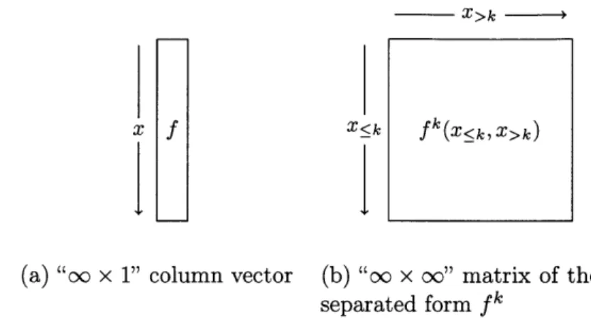
Two such interpretations are provided in Figure 1. The first interpretation, shown in Figure2-X>k -4
X f -<k fk'(x~k, X>k)
(a) "oo x 1" column vector (b) "oo x oo" matrix of the
separated form fk
Figure 2-1: Vector and matrix interpretations of scalar-valued functions
la views
f
as vector with an (uncountably) infinite number of rows, where each "row" is indexed by x E X. This interpretation motivates the inner product between scalar-valued function as a continuous analogue to the inner product between discrete vector, e.g., let g : X-+ R, then(f, g) = f(x)g(x)dx,
where the sum of the discrete inner product is effectively "replaced" with an integral for the continuous inner product.
A second interpretation of a scalar-valued function, shown in Figure 2-1b, is as an "oC x o" matrix obtained through a separated form, or unfolding, of
f
obtained by the variable splittings X<k and X>k. The superscript k will often be added to a function to encourage this interpretation, e.g. fk denotes that the variables are separated after the kth variable. Formally, we have fk : X<k X X>k -+ R wherefk (xzk, X>k) = fk({,... , Xk}, {Xk+1, - ,Xd}) = f(Xi, ... , Xd). (2.1)
In this interpretation, the rows of the "matrix" are indexed by X<k E 9
<k and the columns are indexed by X>k E X>k.
Formally, a vector-valued function F : X - R", where n E Z+, is a map from X to a vector with n elements, and it is denoted by an uppercase letter. Analogously to the scalar-valued function case, various "vector" and "matrix" interpretations of F are useful. These interpretations arise from viewing a vector-valued function as an array
of scalar-valued functions. Consider a set of n scalar-valued functions
fi
: - R. Then, the i-th output of F can be indexed according toF[i](x) = fi(x), i = 1, ... , n.
The particular interpretation of a vector-valued function depends on the arrangement of the scalar-valued functions. Three visualizations that are important in this work are provided in Figures 2-2 and 2-3. The first interpretation of a vector-valued function
(1,x)
(2X)
(n, x)
if
1 2n
"oc x 1" column vector 2-2: Vector-valued functions
(b) "oo x n" quasimatrix
as vectors and matrices in continuous linear
al-provided by Figure 2-2a is that of a vector with an infinite number of elements. This vector is formed by the concatenation, or vertical stacking, of the scalar-valued functions
fi.
Due to this concatenation, the rows of this vector are now indexed by a tuple (i, x) E {1, . . ., n} x X. This viewpoint motivates the following definition foran inner product. Let G : X --+ Rn be another vector-valued function whose outputs are referred to by the scalar-valued functions gi : X -+ R, then the inner product between F and G is
n n
(F, G) = (F[i](x), G[i](x)) = (fi(x), gi(x)).
i=1 i=1 (2.2)
fl
1 f2 ...Af
(a) Figure gebra X f,The second interpretation of a vector-valued function is that of an "Do x n"
quasi-matrixi, and is shown by Figure 2-2b. The rows of the quasimatrix are indexed by x E X and the columns are indexed by i = 1,.... , n such that each column corre-sponds to the scalar-valued function
fi.
This interpretation of a vector-valued function arises in the context of continuous matrix factorizations such as the continuous LU or continuous QR decomposition of Sections 2.2 and 2.2, respectively.The final interpretation comes from considering separated forms, or unfoldings, of vector-valued functions. These unfoldings Fk are obtained by splitting the input space at the kth input. Thus, an unfolding Fk : &Ck X X>k -+ Rn takes values
Fk (X<k, X>k) = F k({Xi,.. ., 4}, {Xk+1, ... , Xd}) = F(xi, ... , Xd).
A visualization of this representation as an "oo x oc" matrix is provided in Figure 2-3.
In Figure 2-3, the rows are indexed by an index-value pair (i, k) where i = 1, ... , n X>k -(1, X~k) 'I X~k - _ fk (X~k, X>k)_ _ _ (2,Xsk) X<k fk(x<k,x>k) (iX~k) ~ 4 ______
I
(n, X k) X~k fk (X~k, X>k)Figure 2-3: Visualization of unfoldings Fk of a vector-valued function F
and the columns are indexed by X>k. This interpretation will be used heavily when
considering the skeleton decomposition of a vector-valued function in Section 2.3.1.
Formally, a matrix-valued function F : X -- R" n , where n, m E Z+, is a map
from X to a n x m matrix, and is denoted by an upper-case, calligraphic, non-bold letter. The matrix-valued function can be visualized as an array of vector-valued 'Called a quasimatrix in, e.g., [4,118] because it corresponds to a matrix of infinite rows and n columns
1 2 - m
I I
I I
jy172 ___
Figure 2-4: Visualization of a matrix-valued function F.
functions F : -+ R' for
j
= 1 ... m according toF= [F F2 ... Fm] such that F[:,j](x) = F(x), j = 1,...,m.
If we consider that each F is itself an array of scalar-valued functions fij : X R for
i = 1, ... , n and
j
= 1, ... , m then the matrix-valued function can also be visualized as a two-dimensional array of scalar-valued functions given byfn,1 I ... fn,m _
In Chapter 3, we show that the cores of a function represented in the function-train format are matrix-valued functions, and this interpretation of a matrix-valued function becomes important.
We can interpret the matrix-valued function as a matrix with an infinite number of rows and m columns, as shown in Figure 2-4. Each "row" of this matrix is indexed
by the pair (i, x) where i E
{1,
... , n} and x E X. Each column refers to the vector-valued function F and is indexed by a discrete variablej
= 1, ... , m.The inner product between F and another matrix-valued function G :
X
- Rnxm is defined as(F, G) = E (F[i, j](x), [i, j](x)) = (fij (, gi, (x)). (2.3)
This inner product can be interpreted as the inner product between two flattened vector-valued functions, and it is analogous to the square of the Frobenius norm of a matrix.
2.1.2
Multiplication
In addition, we define products between arrays of functions (vector- and matrix-valued functions) and arrays of scalars (vectors and matrices), as shown in Table 2.1.
_1_F : X-+ R___ F_:
K
Rmxng = Fx <=
n G = Fx
v E g(x) = Zv[i]F[i](x) G[i](x) = F[i,:](x)x
i=1_______________________
A E Rnxi G = FA FA
G[i] (x) = FA[:, i]
g[i, ij](x)
= F[i, :] (x)A[:, j]Table 2.1: Product of a vector-valued function and a vector (top left); a vector-valued function and a matrix (bottom left); a matrix-valued function and a vector (top right); a matrix-valued function and a matrix (bottom right).
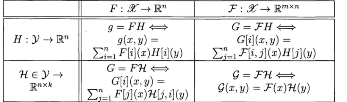
We also define products between functional elements. Let X c Rd and Y C R where d2 E Z+. Then products between vector-valued or matrix-valued functions on
these domains yield vector-valued or matrix-valued functions on the space X x Y. Notation and a summary of these operations are provided in Table 2.2. We now
F : X a Rn _T: X M Rmxn g = FIH ->G = FH H: Y -+ R g(X, y) = [i](x, y)= i=
1
F[i](x)H[i](y) 1 x [i, j] (x)H[j](y) x E n -+ G[i (x y) - x )= F x' j= I F [j] () 7 [, i] (y)Table 2.2: Product of two vector-valued functions (top left); a vector-valued function and a matrix-valued function (bottom left); a matrix-valued function and a vector-valued function (top right); two matrix-vector-valued functions (bottom right).
2.2
Continuous matrix factorizations
Approximating a black box tensor in tensor-train format requires performing a se-quence of standard matrix factorizations. Our continuous framework requires con-tinuous equivalents of these factorization for the elements of concon-tinuous linear al-gebra, scalar-valued functions, vector-valued functions, and matrix-valued functions, described above.
The LU and QR factorizations and the singular value decomposition (SVD) of a vector-valued function are primary ingredients of any continuous numerical linear al-gebra package such as Chebfun [101] or ApproxFun [92]. For vector-valued functions of one variable, these decompositions are discussed in [4]. Computing these decom-positions often requires continuous analogues of standard discrete algorithms. For example, Householder triangularization may be used to compute the QR decompo-sition of a vector-valued function [119]. Extensions of these algorithms to functions of two variables are described in [118]. We will use these bivariate extensions as building blocks for our higher dimensional constructions, and we discuss the relevant background.
LU decomposition
To extend the cross approximation and maxvol algorithms to the continuous set-ting, we will require the LU decomposition of a vector-valued function. The key
components of this decomposition are a set of pivots {z1, z2,... , zn}, zi E X, and a vector-valued function L =
[
l f2 ... n] (here written as a quasimatrix, with scalar-valued functions fi) that is "psychologically" lower triangular [118].A psychologically lower triangular vector-valued function is defined such that
col-umn k has zeros at all zi for i = 1, ... , k - 1. Furthermore, if fi(zi) = 1, then L is unit lower triangular. Finally, if |ik(X)l |fk(Zk)| for all x E X, then L is diagonally maximal. Using these definitions we recall the definition of an LU decomposition of
a vector-valued function [4,118]:
a vector-valued function. An L U factorization of F is a decomposition of the form
F = LU, where U C R"'< is upper triangular and L : X --+ Rn is unit lower triangular and diagonally maximal.
The LU factorization may be computed using Gaussian elimination with row piv-oting according to the algorithm in [118].
We can extend this definition of an LU factorization to matrix-valued functions. In
particular, the decomposition will result in a set of pivots {(ii, zi), (i2, z2), ... , (in, zn)}; a psychologically lower triangular matrix-valued function L; an upper triangular ma-trix U. The definition of the pivots is motivated by viewing L : X -+ Rm"' as
collection of n columns [L[:, 1] ... L[:, n]], where each column is a vector-valued func-tion to be interpreted as an "oc x 1" vector, as described in Section 2.1. Each pivot is then specified by a (row, value) tuple. A lower triangular matrix-valued function is defined such that L [:, k] has zeros at all {(i1, z1), (i2, z2), . .(ik-1, zk_1)]; that is, L[:, 1]
has no enforced zeros, L[:, 2] has a zero in row i1 at the value zj, L[:, 3] has zeros at
(ii, zi) and (i2, z2), etc. Furthermore, if L[ik, k](zk) = 1 then L is called unit lower
triangular, and if IL[i, k](x)I < L[ik, k](zk)I for all x E Xand for all i E 1, ... , M}, then L is diagonally maximal. Using these notions we define an LU decomposition of a matrix-valued function.
Definition 2 (LU factorization of a matrix-valued function). Let F : X -+ R' n be
a matrix-valued function. An LU factorization of F is a decomposition of the form F = LU where U C Rxfl is upper triangular, and L : X 4 Rm"' is unit lower
triangular and diagonally maximal.
We also implement the LU decomposition of a matrix-valued function using Gaus-sian elimination with row-pivoting.
QR decomposition
Another decomposition that will be necessary for function-train rounding and for the cross approximation of multivariate functions is the QR factorization of a quasimatrix.
Definition 3 (QR factorization of a vector-valued function
[4]).
Let F : X -+ R nbe a vector-valued function. A QR factorization of F is a decomposition of the form F = QR, where the vector-valued function
Q
: X - R' consists of n orthonormalscalar-valued functions and R E Rx is an upper triangular matrix.
This QR factorization can be computed in a stable manner using a continuous extension of Householder triangularization [119]. In this dissertation, we also require the QR decomposition of a matrix-valued function.
Definition 4 (QR factorization of a matrix-valued function). Let F : X -+ Rmxn
be a matrix-valued function. A QR factorization of F is a decomposition of the form F = QR, where the columns of Q : X -+ R"X are orthonormal vector-valued
functions and R
e
R.x. is an upper triangular matrix.Since we have defined the inner product of vector-valued functions in (2.2) and therefore are able to take inner products of the columns of F, we can also compute this factorization in a stable manner using Householder triangularization. We can consider the ranks of both vector-valued and matrix-valued functions as the number of nonzero elements of the diagonal of R.
Singular value decomposition
Many of our theoretical results will employ the functional SVD.
Definition 5 (Functional SVD). Let Y x Z C Rd and let g : Y x Z -+ R be in L2(y x Z). A singular value decomposition of g is
00
g(y,z) = Z juj (y)v (z), (2.4)
j=1
where the left singular functions uj : Y -+ R are orthonormal in L2(y), the right singular functions vj : Z -+ R are orthonormal in L2(Z) , and a1 o2 ; > 0 are
the singular values.
In practice, the summation in (2.4) is truncated to some finite number of terms
function U : y --+ R' such that U[i] = uj. Similarly, we group the right singular
functions into a vector-valued function V: Z -4 R1, with V[i] = vi. If we also define
S = diag(u,... , o-), then we can write the functional SVD as g = USV. In this form, we say that g is a function that has an SVD rank of r. This notion of the SVD of a function has existed for a while [108,112] and is also called the Schmidt decomposition [108]. In general, convergence can be assumed to be in L2(y x Z). As described in [118], when g : [a, b] x [c, d] -* R is also Lipschitz continuous, then the series in (2.4) converges absolutely and uniformly.
The functional SVD is useful for analyzing certain separated representations fk of multivariate functions
f.
For example, in Section 3.2.1 we show that the ranks of our function-train representation are bounded by the SVD ranks of the separatedfunctions fk y x Z -- R, where we put Y = X<, and Z = X,, in the above
definition.
Next, we present a decomposition similar to the functional SVD, but for vector-valued rather than scalar-vector-valued functions. We call the decomposition an extended SVD, because it shares some properties with the functional SVD, such as a separation rank, and because it decomposes the vector-valued function into a sum of products of orthonormal functions. This decomposition appears in the proofs of Theorems 3 and 4, as well as in the skeleton decomposition of a multivariate function described in Section 3.3.1.
Definition 6 (Extended SVD). Let 3(x T c R' and let G : Y x _ - R' be a vector-valued function such that G[i] E L2(& x 2) for i = 1, ... , n. A rank r extended
SVD of G(y, z) is a factorization
r
G[i](y, z) =Zoj U [i](y)vj (z), (2.5)
j=1
where the left singular functions Uj : -* R' are orthonormal2 and vector-valued,
the right singular functions vj : _ -÷ R are orthonormal and scalar-valued, and -l ;> o2 ;> -- -> 0 are the singular values.
2Orthonormality
We can combine the left singular functions to form the matrix-valued function U : -+ R" where U[:,j] = Uj, and as in the functional SVD, we can group the right singular functions to form the vector-valued function V : Y - R' such that
V[j] = v3. If we also gather the singular values in a diagonal matrix S, then the
extended SVD can be written as G = USV.
The main interpretation of this decomposition is that G contains n functions that have the same right singular vectors and different left singular vectors. We will exploit two properties of this decomposition for the proof of Theorem 1. The first is the fact that for any fixed 2, the vector-valued function G(y) = G(y, 2) can be represented as a linear combination of the columns of U(y). Second, for any fixed
y
and column2, the function (z) = G[i](y, z) can be represented as a linear combination of the columns of V.
Again, in the case of functions of more than two variables, the extended SVD can be applied to the function's k-separated representation. In particular, if X c R d and we have a vector-valued function F : X -+ R" , then we can consider the extended
SVD of the separated form F : 3x _T-+ R, where we put G = F, 9= 9 <k, and
-= a>k in the definition above.
2.3
Skeleton decomposition and cross approximation
In Section 3.2.1 we show that the FT representation of a function