Three-dimensional GIS cartography applied to the
study of the spatial variation of soil horizons
in a Swiss floodplain
M.L. Mendonc
¸a Santos
a,), C. Guenat
b, M. Bouzelboudjen
c,
F. Golay
da
EMBRAPA-Centro Nacional de Pesquisa de Solos, R. Jardim Botanico 1024,ˆ
22.460-000 Rio de Janeiro-RJ, Brazil
b ´
IATE-Pedologie, Ecole Polytechnique Federale de Lausanne, CH-1015, Lausanne, Switzerland´ ´ ´
c
UniÕersite de Neuchatel, Centre d’Hydrogeologie, Emile-Argand 11 CH-2007,´ ˆ ´
Neuchatel, Switzerlandˆ
d ´
IGEO-SIRS, Ecole Polytechnique Federale de Lausanne, CH-1015, Lausanne, Switzerland´ ´
Abstract
In this study, we propose to establish a framework for the study of the spatial variability of the soils found in the floodplain of the Sarine River and for the visualisation of soil distribution
Ž .
patterns in two- and three-dimensions 2-D, 3-D . This environment is characterised by a large lateral and vertical spatial variability of soils that corresponds to the temporal and spatial variations of the fluvial dynamics of the Sarine. The study was carried out using existing
Ž .
Geographical Information System GIS functions combined with applications specific to soil cartography. This particular GIS cartography is based on the notion of the soil horizon instead of
Ž .
that of the soil diagnostic profile. A Global Positioning System GPS survey was carried out in
Ž .
order to construct a local Digital Elevation Model DEM and to ascertain the spatial coordinates for each of the 181 soil obsevation locations. All data were stored in a GIS database, and both landform modeling and soil cartography was undertaken. GIS, ARCrINFO, and Vertical Mapper for MapInfo were adequate for our linear triangulation interpolation, for contour processing and for the creation of cross-sections as well as the corresponding vertical profiles. These vertical profiles served to illustrate the superposition of soil horizons along any line across the sampled area. A 3-D representation of soil was obtained using the quadratic finite-element method, which is generally employed in geological studies and which we adapted especially for the representation
)
Corresponding author. Tel.: q55-21-274-4999; fax: q55-21-274-5291.
Ž .
E-mail address: [email protected] M.L. Mendonc¸a Santos . Published in Geoderma 97, issue 3-4, 351-366, 2000
of soil horizons. 3-D cartography of this type allows the spatial pattern of a given horizon — including the variation of its thickness, the superimposition of the different soil horizons, the total soil depth, and the number of horizons at any given location — to be followed through space. Our approach, furthermore, facilitates the perception of soil horizons and their juxtarelationships as 3-D objects, and permits the visualisation of the relationships that exist between any given horizon Žor sequence of horizons and the surface topography. In thus enabling the realistic representation. and easy visualisation of the spatial distribution and variability of soils in the landscape, our methodological approach provides a powerful instrument for soil scientists, and a useful decision-support tool for ecosystem management.
Keywords: three-dimensional visualisation; soil mapping; GIS; alluvial soil; Switzerland;
pedo-metrics
1. Introduction
Several authors have already discussed the two main models used in the development of soil cartography: namely, the discrete and the continuous
Ž .
models Baize, 1986; Aubert and Boulaine, 1989; Lark and Beckett, 1998 . Traditional soil cartography is based on the discrete model of soil spatial variability. This assumes that soil characteristics or type change abruptly at soil boundaries. In general, each map unit represents a pedological characteristic that is a constant or unique type of soil. In the latter case, the unit is defined by a
Ž .
‘‘representative soil profile’’ Soil Survey Staff, 1976 . The discrete model is not usually realistic because natural boundaries in landscape tend to be gradual rather than abrupt. Nevertheless, at intermediate mapping scales, traditional soil
Ž
cartography can offer the appropriate solution Voltz and Webster, 1990; .
Lagacherie et al., 1995 , because soil boundaries can be easily identified by Ž
changes in the landscape break of slope, changes of parental material, vegeta-.
tion, etc. .
The continuous model provides another way of approaching soil spatial variability. This assumes that soil characteristics vary gradually through space. Among the available techniques that facilitated the use of continuous model, geostatistics is the one which has been seen as most appropriate for use in soil
Ž
science Voltz and Webster, 1990; Voltz et al., 1997; De Gruijter et al., 1994; .
Qian and Klinka, 1995 . To address the continuum aspect of soils, FitzPatrick Ž1986 recommended that soil cartography be based on the notion of horizons. rather than on that of soil profiles. Cartography by soil horizon despite being based on the discrete model of spatial variation, facilitates the perception of soil as it appears. This approach has three advantages. First, it considers soil as a
Ž .
three-dimensional 3-D body. Secondly, it takes the spatial variability of soil horizons into consideration. Thirdly, it allows the superpositional pattern of the soil horizons to be analysed. These advantages have been discussed by several
Ž
.
King, 1986; Pedro, 1989; Ruellan et al., 1989 . Up until now, soil cartography by horizons has mainly been applied to tropical soils or soils whose horizons are
Ž .
clearly differentiated Bocquier, 1973 .
Ž .
Moreover, Geographical Information System GIS technology has greatly facilitated the 3-D visualisation of soil as a continuous surface. Visualisation techniques such as these have been developed recently in the field of geology ŽBouzelboudjen and Kimmeier, 1998; Houding, 1994 . By contrast in soil.
Ž
science, this kind of representation is in its infancy Ameskamp, 1997; Benz, .
1995; Heijs et al., 1996; Pereira and FitzPatrick, 1998 .
In alluvial soils, the sequence of horizons at a given location is the result of sedimentation and in-situ pedogenesis; these two processes overlap but
inheri-Ž .
tance is predominant Gerrard, 1992; Mendonc
¸a Santos et al., 1997a . This
absence of genetic features in soil profiles, combined with the horizontal and vertical variability of textural configuration of alluvial soils cannot be correctlyŽ
described by the method based on soil diagnostic profiles Finkl, 1980; Gerrard, .
1992 . The horizon approach would seem to describe the complexity and variability of these soil profiles better.
Our aim here is to propose a GIS cartographic framework in order to map and study the spatial variability and distribution pattern of soil horizons in a floodplain, and to represent soil as a continuum in 3-D.
The research was carried out using some existing GIS functions along with applications specifically developed for digital soil horizon cartography. The application of the methodology to a floodplain is justified by the fact that
Ž
floodplain soils possess a high degree of spatial variability both lateral and .
vertical due to the inheritance process, which is extremely difficult to reveal by the classical approach.
2. Material and methods
2.1. Study area
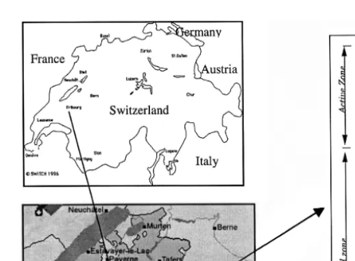
The floodplain is located along the River Sarine near Fribourg in Switzerland ŽFig. 1 . It is about 750 m above sea level. The area under examination covers. approximately 1 ha. A detailed description of the site has already been published ŽMendonc
¸a Santos et al., 1997a,b .
.2.2. Methodology
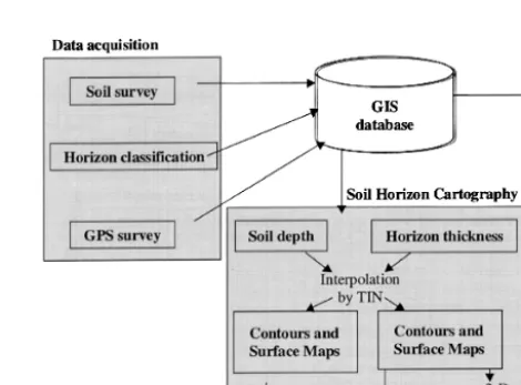
The research was carried out using existing functions in GIS software ŽARCrINFO and Vertical Mapper of Map Info with specific applications to. soil horizon cartography. Fig. 2 illustrates the three principal parts of the
Fig. 1. Location of the study site.
methodology supported by a GIS database: data acquisition, landform modeling, and soil horizon cartography.
2.2.1. Data acquisition
Ž .
A total of 181 points were surveyed using a pedological core sampling drill. Ž
The sampling network was a regular grid 5 m in EW direction and 10 m in SN .
direction . The following properties were recorded for each point: total depth Žthe bottom limit is the D horizon s strand with calcareous pebbles , number of. horizons, thickness and field texture of each horizon.
In addition, the following properties were determined for the topsoil: Ø organic matter content, determined by combustion at 6008C;
Ø presence or absence of coarse material — gravel and pebbles, ) 2 mm; Ø structure — grade, class, and type — according to the Soil Survey Manual
ŽSoil Survey Staff, 1976 ; and.
Ø the presence of carbonates, detected in the field by HCl effervescence. Horizon nomenclature was allocated according to the ‘‘Referentiel Pedolo-
´ ´
´
Ž .
gique 1995’’ A.F.E.S., 1995 . In addition, topsoil texture and structure were used for the identification of the different horizons. In order to be able to
Fig. 2. Diagrammatic representation of the methodology.
construct our soil model, we were obliged to impose an order of horizon position that corresponded to our data set, the assumption being that this order was honoured at unobserved locations.
Ž .
A Global Positioning System GPS survey was carried out to determine the
Ž .
co-ordinates X, Y, Z of each soil survey point to a precision of 50 cm in the horizontal plane and 2 cm in the vertical. All data were stored in a GIS database ŽInfo of ARCrINFO . Table 1 shows an example of these data entries..
2.2.2. Landform modeling
The data from the GPS survey were interpolated using a Triangular Irregular
Ž . Ž .
Network TIN and from this a Digital Elevation Model DEM was built. This technique allows for the surface of each triangle to pass exactly through each
Ž .
measured data value. According to Bonham-Carter 1994 , this approach is the most appropriate one where data are known to have relatively small margins of error. We believe this was the case for our survey.
2.2.3. Soil cartography
The characteristics of our data set — regular grid, dense sampling, and relatively precise measurements — made the use of the TIN interpolation technique particularly appropriate. The 3-D soil cartography by horizons was
Ž .
Table 1 Database entries for horizon thickness ) Ž. Ž. Ž . Site Soil id X m Y m Z surface Horizon thickness cm Ž. number msm Ž . Ž. Ž . Ž . Ž. Ž . Ž . Ž. Ž . Ž . Ž. Aca Jp sl M s Jp ls IIJp sl IIM s IIJp ls IIIJp sl IIIM s IVJp sl Jp l IVM s 1 T12S0b 571161.9315 151168.5340 747.6490 10 15 40 0 0 20 0 0 0 0 15 0 2 T12S1 571156.2130 151170.3250 747.9025 20 0 30 0 0 0 0 0 0 0 0 0 3 T12S1b 571151.3005 151171.9975 748.1160 10 0 50 0 0 25 0 0 0 0 15 0 4 T12S2 571146.7775 151173.7245 748.1895 17 3 0 0 0 0 0 0 0 0 0 0 5 T12S2b 571142.0255 151175.2765 748.2325 15 0 0 0 0 0 0 0 0 0 0 0 6 T12S3 571136.9065 151176.7745 748.2280 18 20 0 0 0 0 0 0 0 0 0 0 7 T12S3b 571132.5110 151178.0635 748.2470 10 0 15 0 0 0 0 0 0 0 0 0 8 T12S4 571127.7810 151179.7580 748.0235 15 23 0 0 0 0 0 0 0 0 0 0 9 T12S4b 571123.0855 151181.1345 747.8785 10 50 0 0 0 0 0 0 0 0 0 0 ... ... ... ... ... ... ... ... ... ... ... ... ... ... ... ... ... ... ... ... ... ... ... ... ... ... ... ... ... ... ... ... ... ... ... ... ... ... ... ... ... ... ... ... ... ... ... ... ... ... ... 181 L0S14 571191.0528 151295.9160 746.6770 6 0 22 0 4 18 0 5 7 0 0 0 ) Ž. Ž . Horizon designations, Aca, Jp sl , etc., follow A.F.E.S. 1995 . Referentiel pedologique. ´´ ´
bottom of each horizon were calculated with basis on the surface elevation value, measured by GPS and the horizon thickness. Secondly, these values were interpolated and contour processing was applied to create isolines contouring the soil survey points. Thirdly, maps with both isolines and filled contour areas were generated in 2-D.
Based on the corresponding grids of the 2-D maps and using the ‘Profiling’ procedure in ARCrINFO, or alternatively using the ‘Cross-section’ procedure
Ž .
in Vertical Mapper MapInfo software, cross-sections could be generated along any line traversing the sample area.
Finally, a 3-D volume model was carried out in order to represent soil as a continuum in the landscape. This was achieved using a quadratic finite element
Ž .
method, the Kiraly’s Fen Code Kiraly, 1985 adapted to soil modeling. The 2-D
´
surface network is vertically replicated at each soil horizon to obtain a 3-D finite element network. It means that each sample point is really represented by a vertical edge of the 3-D network.In the finite-element method, the unknown function is approximated over a subset of the entire global domain by using interpolation functions. In the present paper, only linear interpolation functions are employed. The entire model domain must be discretised into 1-D, 2-D, or 3-D elements. The program allows for the use of either triangles or rectangles for 2-D elements and either tetrahedra, triangular prisms, or cubes for 3-D elements. These elements may undergo further deformation. The number of element shapes allows for consider-able flexibility in designing for example, a 3-D network for analysing water and
Ž .
transport in highly heterogeneous porous media Eisenlohr et al., 1997a,b . In this paper, the post-processing routine allows the possibility of creating a series of cross-sectional planes or 3-D block diagrams.
3. Results and discussion
Fig. 3 illustrates the different steps for building a DEM: the soil survey points
Ž .
and the TIN network mesh Fig. 3a ; contours, the isolines of contour elevation ŽFig. 3b ; and a block diagram of the DEM in so-called 2.5-D Fig. 3c . The. Ž . DEM constructed in this way allows the visualisation of local differences in
Ž .
topography that would not be possible with an ordinary DEM 1:25 000 . On our site, three areas are distinguished. The highest area, which corresponds to an old island and its extension that is easily visible in the middle of the site. Secondly, the intermediate zone situated on the left side of the site. Thirdly, the lowest
Ž
area, a depression on the right side of the site close to the river, which is not .
shown here .
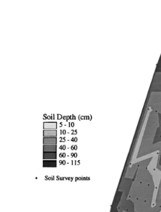
Fig. 4 shows the spatial pattern of soil depth. The thinnest profiles are to be found in the highest areas, while the thickest ones are in the depression.
Ž. Ž . Ž . Ž. Fig. 3. DEM of the study site. a The triangulated network TIN that honours each soil survey point; b the elevation contours of the site; c the block Ž. diagram of the DEM 2.5-D ; bright s the top, dark s depression.
Fig. 4. Map of total soil depth.
Horizon thickness was mapped in 2-D for each of the 12 horizons. The maps Ž . of Fig. 5 illustrates the thickness variation of the first three horizons, Aca, Jp sl ,
Ž .
and M s . These maps enable us to:
Ø visualise the spatial distribution pattern of each horizon and the variation of their thickness;
Ø observe the presence or absence of a given horizon at any particular point; Ø compare the spatial distribution patterns of the various horizons.
Ž .
For example, the left-most map shows the A horizon Aca which is present
Ž .
everywhere, while the right-most one depicts the M horizon a sandy horizon , which is present only at some points. The white zones in the middle and right maps signify the complete absence of the horizon in question.
These maps can also be draped on the surface plot of the DEM in order to study the relationships between horizons and surface topography. Nevertheless, the 2-D representation is not capable of integrating all of the soil horizons simultaneously, a necessary requirement for pedogenetic studies. It does consti-tute an indispensable step towards the necessary 3-D representation, however.
Fig. 5. Maps of horizon thickness for the first three horizons.
Some results obtained with the 3-D approach are illustrated in Fig. 6. In the upper left-hand corner of the figure, the DEM shows the location of three
Ž .
cross-sections two perpendicular to the river and one alongside it . The rest of the figure is comprised of the three cross-sections in question. The legend on the right side of the cross-sections indicates the horizon classification. All the soils are ‘‘calcareous FLUVIOSOLS typiques’’, according to the ‘‘Referentiel
´ ´
Ž .
Pedologique 1995’’ A.F.E.S., 1995 .
´
Cross-section L1, which is located close to the river channel, starts from an
Ž .
elevation of 748 m, crosses the depression with a minimum of 746 m and ends
Ž .
at the old island the highest point in the site, at more than 749 m . Although the
Ž .
surface elevation difference relief is small, it constitutes an important factor in the sedimentation process. There are more horizons at the lowest positions than elsewhere. On the old island, at the end of the transect, for example, the soil contains only one horizon. A similar tendency is corroborated in the other cross-sections. This pattern illustrates clearly the influence of river dynamics upon these soil profiles. Soil profiles with several horizons are essentially formed by alluvial deposition in old branches or close to the river channel in bottom areas. By contrast, the thinnest soils from the highest position have been protected from floods. The presence of a given horizon and its thickness provides information about sedimentation processes due to the same flood event. The spatial configuration of one horizon can be explained by relating it to the
Ž .
presence of under-horizon s , without any reference to the present-day topogra-phy. Thus, the sedimentation processes are easier to reconstruct. For example,
Ž .
the central part of the longitudinal profile L1 demonstrates the past existence of two distinct geomorphological sectors, which are characterised by different sedimentary sequences of horizons. These sectors were subsequently
intercon-Ž .
nected by fluvial dynamics presence of the same horizons and the past topographical variation has been attenuated. This cartographic approach is useful for identifying the two processes that result in alluvial soils: sedimentation and in-situ pedogenesis. As soil units are very difficult to define and to delimit —
Ž .
because all soil profiles belong to the same class calcareous FLUVIOSOLS and because they mainly differ in number and thickness of horizon and vary within a short distance — a more classical approach would have been inappro-priate.
Ž .
The 3-D representation Fig. 7 shows the soil as a volume in space and conserves the advantages of a cross-sectional representation. It contains the same information but it presents them in a volumetric view and allows several cuts, following different perspectives, to be made simultaneously. This provides a greatly increased clarity and simplicity of view, thus constituting a valuable perceptive and didactic tool for the visualisation of soil variation.
For pedological studies, and particularly those concerning alluvial soils, GIS-cartography such as this — allowing the representation of soil by horizon, in 3-D — constitutes a useful improvement over current approaches. It is a
Fig. 6. DEM image showing the location of cross-sections and the corresponding vertical profiles of soil horizons.
Ž . Fig. 7. 3-D soil volume model sun azimuth: N at 608, tilt: 308, vertical exaggeration: 10= . The
Ž . Ž .
vertical nodes of the network correspond to the soil survey points. a The whole site; b three transverse cuts.
useful tool to show how the soil distribution patterns in our study are clearly due to the influence of fluvial dynamics.
This approach has permitted us to observe that the sequence and thickness of
Ž .
the horizons varies over short distances "50 cm , thus elaborating different patterns of change. This could be explained as a consequence of the overlapping of the different factors that influence the sedimentation process, e.g. topogra-phyrgeomorphology, distance to the river channel, and so on.
4. Conclusions, limitations and future improvements
3-D GIS cartography based on soil horizons offers a number of advantages over more traditional cartographic techniques. The only necessary classification is related to horizon definition. In addition to this, however, the use of a GIS
permits a more flexible approach, particularly when considering the type and number of horizons to be mapped and the choice of cross-sections to be generated. Furthermore, our cartographic approach allows the calculation of horizon volumes. Such calculations could be helpful to pedogenetic explanations Žintensity of flood originating a given alluvial deposit , soil properties water or. Ž
. Ž
pollutant storage capacity or to plan landscape management sediment extrac-.
tion for example . Our 3-D GIS representation permits an easier visualisation of the spatial distribution and variability of soil. The methodology is particularly appropriate to the mapping of high spatial variability soils. Our research has demonstrated the undeniable utility of GIS technology for soil scientists, for the facilitation of data-set management, for spatialisation, analysis, visualisation, and mapping in an interactive way. The current model assumes a fixed sequence of horizons, the implications of this assumption needs to be investigated further. Future improvements will also focus on the use of geostatistical techniques in order to quantify the spatial variability of these soils, and uncertainties associ-ated with interpolation. Finally, our GIS-assisted cartography associassoci-ated with thematic maps could provide a useful decision-support tool for the management of ecosystems.
Acknowledgements
The authors would like to thank Denis Baize for his suggestions on the pedological part of this work. Thanks are also extended to Laszlo Kiraly of the
´
´
´
Neuchatel University for modifying the Kiraly’s Fen Codes program to ourˆ
pedological application.References
´
A.F.E.S., 1995. Referentiel Pedologique. Collection Techniques et Practiques. INRA Editions,´ ´ ´ ´
Paris, 332 pp.
Ameskamp, M., 1997. Three-Dimensional Rule-based Continuous Soil Modelling. PhD Thesis. Christian-Albrechts-Universitat, Kiel, 206 pp.¨
Aubert, G., Boulaine, J., 1989. Contributions de certains pedologues franc´ ¸ais a l’evolution des` ´
concepts pedologiques utilises en cartographie. Science du Sol 27, 395–411.´ ´
Baize, D., 1986. Couvertures pedologiques, cartographie et taxonomie. Science du Sol 24,´
227–243.
Benz, R., 1995. Essai d’approche tridimensionnelle de la couverture pedologique: application a´ `
Ž .
trois stations d’etude dans la region du col du Marchairuz Haut-Jura Vaudois . Uni. Neuchatel,´ ´ ˆ
Institut de Botanique, Laboratoire d’Ecologie Vegetale, Neuchatel.´ ´ ˆ
Bocquier, G., 1973. Genese et Evolution de Deux Toposequences de Sols Tropicaux du Tchad.` ´
Interpretation Biogeodynamique. ORSTOM 62, OSRTOM, Paris, 350 pp.´ ´
Bonham-Carter, G.F., 1994. Geographic Information Systems for Geoscientists: Modeling with GIS. Pergamon, Ontario, Canada, 398 pp.
Boulet, R., Humbel, F.X., Lucas, Y., 1982a. Analyse structurale et cartographie en pedologie II.´
Cahiers de l’ORSTOM, Ser. Ped. XIX, 323–339.´ ´
Boulet, R., Chauvel, A., Humbel, F.X., Lucas, Y., 1982b. Analyse structurale et cartographie en pedologie I. Cahiers l’ORSTOM, Ser. Ped. XIX, 309–321.´ ´ ´
Boulet, R., Curmi, P., Pellegrin, J., Queiroz-Neto, J.P., 1989. Distribution spatiale des horizons dans un versant: apport de l’analyse de leurs relations geometriques. Science du Sol 27, 53–56.´ ´
Bouzelboudjen, M., Kimmeier, F., 1998. GIS vector and raster database, advanced geostatistics and 3-D groundwater flow modelling in strongly heterogeneous geologic media : an integrated approach, The 18th Annual ESRI User Conference. ESRI, San Diego, CA, USA.
Ž .
de Gruijter, J.J., Webster, R., Myers, D.E. Eds. , 1994. Special Issue on Pedometrics. Geoderma 62 Elsevier, Amsterdam, 326 pp.
Eisenlohr, L., Kiraly, L., Bouzelboudjen, M., Rossier, Y., 1997a. Numerical simulation as a tool´
for controlling the interpretation of karst spring hydrographs. Journal of Hydrology 193, 306–315.
Eisenlohr, L., Bouzelboudjen, M., Kiraly, L., Rossier, Y., 1997b. Numeric versus hydrological´
and statistical modelling of natural response of a karst hydrogeological system. Journal of Hydrology 202, 244–262.
Finkl, C.W.J., 1980. Statigraphic principles and practices as related to soil mantles. Catena 7, 169–194.
FitzPatrick, E.A., 1986. Soils — Their Formation, Classification and Distribution. Longman, Essex, England, 353 pp.
Gerrard, J., 1992. Soil Geomorphology — An Integration of Pedology and Geomorphology. Chapman & Hall, London, 269 pp.
Girard, M.-C., 1983. Recherche d’une modelisation en vue d’une representation spatiale de la´ ´
couverture pedologique: application a une region des plateaux jurassiques de Bourgogne.´ ` ´
Departement des Sols, No. 12. Institut National Agronomique Paris-Grignon, Paris, 430 pp.´
Girard, M.-C., 1989. La cartographie en horizons. Science du Sol 27, 41–44.
Girard, M.-C., Aurousseau, P., King, D., Legros, J.-P., 1989. Apport de l’informatique a l’analyse`
spatiale de la couverture pedologique et a l’exploitation des cartes. Science du Sol 27,´ `
335–350.
Heijs, A.W.J., Ritsema, C.J., Dekker, L.W., 1996. Three-dimensional visualization of preferential flow patterns in two soils. Geoderma 70, 101–116.
Houding, S.W., 1994. 3D Geoscience Modeling. Springer, Berlin, 309 pp.
King, D., 1986. Modelisation Cartographique du Comportement des Sols. INRA, Paris, 243 pp.´
Kiraly, L., 1985. FEM 301- A Three Dimensional Model for Groundwater Flow Simulation.´
NAGRA Technical Report 84-49. Baden, Switzerland, 96 pp.
Lagacherie, P., Legros, J.-P., Burrough, P.A., 1995. A soil survey procedure using the knowledge on soil pattern of a previously mapped reference area. Geoderma 65, 283–301.
Lark, R.M., Beckett, P.H.T., 1998. A geostatistical descriptor of the spatial distribution of soil classes, and its use in predicting the purity of possible soil map units. Geoderma 83, 243–267. Mendonc¸a Santos, M.L., Guenat, C., Thevoz, C., Bureau, F., Vedy, J.-C., 1997a. Impacts of embanking on the soil-vegetation relationships in a floodplain ecosystem of a pre-alpine river. Global Ecology and Biogeography Letters 6, 339–348.
Mendonc¸a Santos, M.L., Guenat, C., Thevoz, C., Bureau, F., 1997b. Modifications d’une zone alluviale suite a l’endiguement. approche methodologique. Geomorphologie: Relief, Processes,` ´ ´
Environment 4, 365–374.
Pedro, G., 1989. L’approche spatiale en pedologie: fondement de la connaissance des sols dans le´
milieu naturel- reflexions liminaires. Science du Sol 27, 287–300.´
Pereira, V., FitzPatrick, E.A., 1998. Three-dimensional representation of tubular horizons in sandy soils. Geoderma 81, 259–303.
Qian, H., Klinka, K., 1995. Spatial variability of humus forms in some coastal forest ecosystems of British Columbia. Annales des Sciences Foresieres 52, 653–666.
Ruellan, A., Dosso, M., Fritsch, E., 1989. L’analyse structurale de la couverture pedologique.´
Science du Sol 27, 319–334.
Soil Survey Staff, 1976. Soil Taxonomy. Agricultural Handbook 436 US Government Printing Office, Washington, DC.
Voltz, M., Webster, R., 1990. A comparison of kriging, cubic splines and classification for predicting soil properties from sample information. Journal of Soil Science 41, 473–490. Voltz, M., Lagacherie, P., Louchart, X., 1997. Predicting soil properties over a region using
sample information from a mapped reference area. European Journal of Soil Science 48, 19–30.