Sub-Ocean: Subsea Dissolved Methane Measurements Using an Embedded Laser Spectrometer Technology

HAL Id: hal-01913459

https://hal.archives-ouvertes.fr/hal-01913459

HAL is a multi-disciplinary open access archive for the deposit and dissemination of sci-entific research documents, whether they are pub-lished or not. The documents may come from teaching and research institutions in France or abroad, or from public or private research centers.

L’archive ouverte pluridisciplinaire HAL, est destinée au dépôt et à la diffusion de documents scientifiques de niveau recherche, publiés ou non, émanant des établissements d’enseignement et de recherche français ou étrangers, des laboratoires publics ou privés.

Sub-Ocean: Subsea Dissolved Methane Measurements

Using an Embedded Laser Spectrometer Technology

Roberto Grilli, Jack Triest, Jérôme Chappellaz, Michel Calzas, Thibault

Desbois, Pär Jansson, Christophe Guillerm, Benedicte Ferré, Loic

Lechevallier, Victor Ledoux, et al.

To cite this version:

Roberto Grilli, Jack Triest, Jérôme Chappellaz, Michel Calzas, Thibault Desbois, et al.. Sub-Ocean: Subsea Dissolved Methane Measurements Using an Embedded Laser Spectrometer Technology. En-vironmental Science and Technology, American Chemical Society, 2018, 52 (18), pp.10543 - 10551. �10.1021/acs.est.7b06171�. �hal-01913459�

1

Sub-Ocean: Subsea Dissolved Methane Measurements Using an

Embedded Laser Spectrometer Technology

Roberto Grilli,*,† _{Jack Triest,}† _{Jérôme Chappellaz,}† _{Michel Calzas,}‡ _{Thibault Desbois,}§ _Pär Jansson,∥ Christophe Guillerm,‡ Bénédicte Ferré,∥ Loïc Lechevallier,†,§ Victor Ledoux,† and Daniele Romanini§

† _{Université Grenoble Alpes, CNRS, IRD, Grenoble INP, Université Grenoble Alpes, IGE, F-38000}

Grenoble, France

‡ _{CNRS DT INSU, 29280 Plouzané, France}

§ _{Université Grenoble Alpes, CNRS, LIPhy, F-38000 Grenoble, France}

∥ _{CAGE - Center of Arctic Gas Hydrate, Environment and Climate, Department of Geology, UiT}

University of Norway, N-9019 Tromsø, Norway

*Corresponding Author: Roberto Grilli. Phone: +33 (0) 4 76 82 42 66. E-mail: [email protected].

Corresponding author address: Institut des Géosciences de l’Environnement (IGE), Université Grenoble Alpes, 54 rue Moliére - BP 96, 38400 St. Martin d’Hères, France.

2

Abstract. We present a novel instrument, the Sub-Ocean probe, allowing in situ and

continuous measurements of dissolved methane in seawater. It relies on an optical

feedback cavity enhanced absorption technique designed for trace gas measurements

and coupled to a patent-pending sample extraction method. The considerable advantage

of the instrument compared with existing ones lies in its fast response time of the order

of 30 s, that makes this probe ideal for fast and continuous 3D-mapping of dissolved

methane in water. It could work up to 40 MPa of external pressure and it provides a

large dynamic range, from subnmol of CH4 per liter of seawater to mmol L-1. In this

work, we present laboratory calibration of the instrument, intercomparison with

standard method and field results on methane detection. The good agreement with the

headspace equilibration technique followed by gas-chromatography analysis supports

the utility and accuracy of the instrument. A continuous 620-m depth vertical profile in

the Mediterranean Sea was obtained within only 10 min and it indicates background

dissolved CH4 values between 1 and 2 nmol L-1 below the pycnocline, similar to previous

observations conducted in different ocean settings. It also reveals a methane maximum

at around 6 m of depth that may reflect local production from bacterial transformation

of dissolved organic matter.

1. Introduction

The measurement of dissolved gases in a liquid medium (notably in water) is

essential for different applications, such as environmental monitoring, search for natural

gas reservoirs in the seafloor, deep-sea oil and gas pipeline inspection, monitoring the

activity of bioreactors, safety control of industrial facilities or monitoring water quality

3

focus over the last two decades has been the investigation of the fate of methane hydrate

degassing from the seafloor and its relationship with global warming.1 _{Although methane}

released from hydrate reservoirs in the sediments appears to be mostly oxidized in the

water column (see Ruppel and Kessler 2017 for a recent review), its contribution to ocean

acidification is still under debate.2,3 _{Therefore, a quantitative evaluation of methane fluxes}

from the seafloor in gas hydrate-bearing regions remains needed, as well as the spatial

and temporal dissolved methane evolution along the water column due to aerobic

oxidation, diffusion, and transport. Other important scientific issues also require in situ

measurements of dissolved methane, like the interactions between seasonal thawing of

permafrost and organic transfer through Arctic river systems or methane fluxes from

deep ocean seeps. These devices are also important in the study of microbial methane

production in the oxic waters of oceans and lakes, a source of methane that can be

important for carbon cycling in the aquatic environments and water to air methane

fluxes.4-7

In the last years to decades, knowledge of physical properties of ocean surface water has

been considerably improved thanks to remote (satellite) measurements8,9 _and

near-surface water sampling and analysis. However, three-dimensional distributions of

dissolved gases are far less constrained since marine subsurface environments are more

difficult to access. Parameters such as temperature, salinity, and oxygen are acquired

using instruments such as a CTD (conductivity, temperature, and depth devices) that can

run autonomously and can be implemented in floats, moorings, and gliders.10 _Information

about dissolved trace gases is more commonly extracted using discrete sampling

(employing Niskin bottles) followed by laboratory measurements. This process is time

consuming and provides data with poor spatial and temporal resolution, not adapted for

4

some situations, water samples degassing from the Niskin bottles have been observed

during the ascent, causing a degradation of the samples.11 _{Furthermore, in the case of}

supersaturated samples, outgassing during water sampling is difficult to prevent or

quantify, leading to a possible underestimation of the amount of dissolved gas in deep

waters. For these reasons, in situ instrumentation has more recently been developed, with

the aim to provide more reliable (less sample manipulation) and fast measurements of

dissolved gases. Most of it relies on embedded optical devices or mass spectrometers

(MS). A review on the available sensors has been presented by Boulart et al.12 _discussing

the performances of existing commercial devices and other systems based on membrane

separation, equilibrators, and in situ MS. Apart from in situ MS,13 _{the other approaches}

have limited response time (on the order of tens of minutes and mainly limited by the

extraction method), making these devices less suitable for fast 3D mapping applications.14

In situ MS provide acceptable sensitivity and response time, but are often not sensitive

enough for background concentrations. Their deployments as a stand-alone instruments

are limited by the payload, power consumption, and cost. Furthermore, application of MS

can suffer from interferences due to the presence of water vapor in the analyzed gas

mixture, while optical techniques can work in spectral regions where water absorption is

weak. If isotopic ratio MS (IRMS) are currently not compact enough to be embedded in

subsea probes, optical spectrometers have already been successfully embedded in subsea

sensors for in situ isotopic analysis, with applications to deep-sea measurements.15,16

Today, optical techniques are largely employed for in situ high resolution measurements

of gas mixtures either directly in the atmosphere (from ground measurements to airborne

monitoring or stratospheric balloons measurements), in ice cores (in the laboratory17 _but

soon also in situ18_{) and finally for measuring dissolved gases in liquids. The use of optical}

5

direct absorption techniques, leading to robust and compact devices with small sample

volume, easy to implement into a specific probe for field applications that require small

sample flow. In this work we used optical feedback cavity enhanced absorption

spectroscopy (OFCEAS),19,20 _{and further information can be found in Morville et al.}21 _The

employment of this technique for dissolved gas measurements leads to advantages such

as multiple species detection and the possibility to avoid interferences such as the

presence of water vapor and other species present in the gas mixture (e.g. other

hydrocarbons).

In this work, we describe the first application of the OFCEAS technique – combined with

a patent-pending gas extraction module22 _{- for in situ real-time measurements of}

dissolved methane in seawater. Measurements have been conducted as a

proof-of-concept in the Mediterranean Sea in July 2014.

2. Materials and Methods

2.1 The in Situ Sensor

The optical instrument used in this study is the SUBGLACIOR spectrometer,18

developed as a drilling probe embedded device for in situ real-time measurements of air

bubbles trapped in Antarctic glaciers.23,24 _{As a new design, it required calibration and}

testing in real environments before deployment to Antarctica, and the Mediterranean

Sea was for us a good compromise (because of temperature fluctuations and increase of

pressure with depth) even though not as extreme as Polar Regions. The spectrometer

was made of an optical part that fits in a tube of 6.3 cm external diameter and 1.3 m long

and an electronic part (8 cm ext. diameter, 1.2 m long). The optical spectrometer, based

6

measuring simultaneously CH4 and δD of H2O. The dissolved air from the extraction unit

(discussed below) was continuously pumped to the optical cavity of the spectrometer.

The internal volume of the cell is less than 20 cm3 _{and provides sample residence times}

< 30 s for optimal running conditions (combination of pressure and total gas flow). The

instrument was equipped with an embedded PC, for processing and storing the data.

Two protocols were implemented in order to communicate with the instrument during

the field campaign. The first one used a wireless connection (ad-hoc network

configuration), providing easy access to the embedded instrument via a PC-PC

communication. The second protocol employed cabled communication, allowing

real-time transfer of data together with remote control of the spectrometer, if necessary.

Extraction of dissolved gases from seawater was performed using a silicon rubber

membrane, for which the technology has previously been described in terms of physical

properties such as adsorption, permeation, and desorption.25-30 _{Existing sensors,}

including commercial instruments from Contros (Kongsberg), Franatech, Los Gatos

Research and Pro-Oceanus, employ membrane extraction for measuring dissolved

gases.31,32 _{Membrane extraction techniques found in the literature rely on gas}

equilibration across the membrane that allows for precise measurements of dissolved

gas concentration, at the cost of slow response time (>20 min).14,33 _{Here, we propose a}

different approach consisting of maintaining the dry side of the membrane at low

pressure, while continuously flushing it with dry “zero” gas. The pressure at the

membrane dry side controls the total flow of dry and wet air through the membrane,

and the system was designed to keep this pressure constant. While the spectrometer

operates at about 20 mbar, the pressure against the dry side of the membrane was

7

Gas permeation through a membrane depends on the solubility in the membrane

itself, followed by diffusion (migration of molecules through the membrane lattice) and

finally evaporation out of the membrane.27 _{It is well known that the partial pressure}

difference of a given gas species controls the diffusion across the membrane and

therefore the response time of the extraction system. Other parameters affecting the

permeation efficiency are the membrane thickness, water flow over the membrane and

ambient temperature: lower thickness, larger flow and higher temperature lead to

higher permeability, and therefore faster response time. With respect to the membrane

properties, a higher temperature increases the free volume as well as the mobility of the

polymer chain, leading to higher diffusivity of gases through the membrane. With

respect to any given gas, higher temperature means higher mobility, diffusivity and

permeability. Water flow and temperature therefore need to be accurately and precisely

controlled for an optimal behavior of the membrane extraction system. Biofouling,

salinity, pressure and pH of the water may also affect the efficiency of the permeability,

but, apart from salinity, this has not been investigated here, and it will require further

investigation.

In our setup, two 10 µm thick polydimethylsiloxane (PDMS) membranes of 56 mm diameter, were mounted face-to-face in a stainless steel housing in order to double the

membrane surface. The membranes were simultaneously flushed with the water sample

using a submersible water pump (Sea-Bird Electronics, SBE 5T) providing a flow of 0.8 L

min-1_{. The membranes were supported by porous bronze frits of 3 mm of thickness}

(Poral, grade 20), providing mechanical strength for the membrane under high pressure

differences. The membrane block was designed to ensure that the water sample

continuously flushed the entire surface of the membranes (a schematic of the membrane

8

The dissolved methane sensor runs on 24 VDC power supply, with 50 W nominal

consumption. During the present study it was powered through an electromechanical

coaxial cable allowing for long-term deployment, but the system can also run on 24 VDC

battery packs. Long-term deployment endurance will be further limited by the gas

storage capacity inside the instrument, and by the carrier gas flow. The instrument was

successfully deployed while measuring continuously for up to 12 h. A CTD unit

(Aanderaa, Seaguard TD262a) was attached to the probe, providing salinity-, water

temperature-, depth-, and dissolved oxygen data.

2.2 The Site of Study

The Sub-Ocean probe was deployed as proof-of-concept onboard the CNRS-INSU

research vessel Téthys II in the northwest part of the Mediterranean Sea on July 12and

13, 2014. Because of adverse meteorological conditions, the deployment was limited to

an area with only 620 m of depth available. The first tests of the instrument were

conducted at ~200 m from Toulon’s harbor (43°6.20 N - 5°56.73 E) for proving its

stability and functioning. Vertical profiles were obtained in an area between Fréjus and

the Gulf of the Napoule, at ~8 km from the coast (43°24.89 N - 7°00.61 E), not far from

the Gulf of Lions. The Gulf of Lions was a target site for measurement of dissolved

greenhouse gases34 _{and sediment core analysis}35 _{because of its particular hydrological}

character, mainly marked by the presence of large fresh water incoming from the Rhone

River (with a flux on the order of 1600 m3 _s-1_).

2.3 The Laboratory Apparatus

The schematic of the laboratory experimental setup is represented in Figure 1. It was

composed of a 14 L, 21 cm diameter, 40 cm high aluminum chamber, containing about 8

9

NaCl (Merck, purity >99.5%) was added for reproducing particular salinity conditions.

Salinity was measured with a digital refractometer (Bellingham and Stanley, 38-51

Aquatic). The temperature of the water in the chamber was stabilized between 2 and

25°C using a water cooling system (RM6, Lauda) and monitored by an immerged

PT1000.The pressure above the water was maintained at atmospheric pressure (~101.3

kPa). The water was continuously bubbled with a gas mixture composed of zero air

(ALPHAGAZ 2, Air Liquide) and synthetic air containing CH4 at concentrations between

0 and 90 ppmv (SAPHIR 90 ppmv of CH4 in air, Air Liquide) by means of a diffuser

installed at the bottom of the chamber. The role of the diffuser was to reduce the

bubbles size and to achieve dissolved gas saturation in a short time. The dilution system

consisted of two mass-flow-controllers (MFC1 and MFC2, Bronkhorst) delivering up to

100 sccm (standard cubic centimeters per minute) of gas. Water circulation was

provided by the SBE 5T pump, ensuring a well mix of water in the chamber. The pump

and the diffuser were positioned at maximum distance from each other to allow the best

homogeneity of the water sample during the measurement and to avoid trapping air

bubbles in the extraction system. The water circulated on the wet sides of the

membranes included in the membrane block (MB, cf SI-3) and dissolved gases were

extracted on the dry side and further transferred to the Sub-Ocean spectrometer. A dry

carrier gas flow (zero air, ALPHAGAZ 2, Air Liquide) was supplied by a 0-10 sccm mass

flow controller (MFCCG) to the dry side of the membrane extraction system, for

continuously flushing the permeated gases from the membrane. This maintained CH4

partial gas pressures at the lowest possible level on the dry side of the membrane in

order to optimize the extraction efficiency and response time. A flowmeter (IQF+,

Bronkhorst) was used for monitoring the total gas flow (composed of the carrier gas

10

the headspace of the calibration chamber was continuously monitored by a laser

spectrometer based on the same principle as the Sub-Ocean instrument, but designed

for laboratory purposes (headspace spectrometer in Figure 1). Ten sccm of the

headspace gas was supplied to the headspace spectrometer, while the overflow was sent

to an exhaust vent. For inter-comparison with the discrete sample technique, water

samples were collected in 115 ml vials. During collection, 1 ml of 1M NaOHwas added in

order to inhibit bacterial activity. The vials were fully filled and closed with butyl rubber

caps and aluminum crimps tops. Subsequently, 5 ml of the samples were replaced with

pure nitrogen (Air Liquide) at atmospheric pressure and 20°C. The samples were

analyzed at the University of Tromsø by gas-chromatography under blind conditions. A

ThermoScientific Trace 1310 GC equipped with a FID and a ThermoScientific TG-Bond

Msieve 5A column was used with hydrogen as carrier gas (10 ml/min). The oven was

operated at a constant temperature of 150°C and the system was calibrated with three

external methane standards at 1.8, 19, and 1800 ppmv. Instrument precision was

estimated based on the standard deviation of replicates, and found to be 4% of

measured methane concentration.

2.4 The calibration in the laboratory

The challenge in quantifying variations in membrane permeability makes

measurements performed by gas-extraction membranes rather uncertain.12 _Therefore,

we paid special attention for calibrating and evaluating the performance of the

instrument under laboratory controlled conditions.

Both spectrometers used in the calibration apparatus (for measuring the headspace

air and the dissolved gases, Figure 1) were calibrated using certified standard gas

(Restek, Scott/Air Liquide 99 ppmv ± 5%). Different concentrations were obtained with

11

1). A linear response over the whole range of concentrations was obtained with a good

agreement between the two devices (slope 1.090 ± 0.0027, R2 _{= 0.99995 in 2015 and}

slope 0.9926 ± 0.003, R2 _{= 0.99989 in 2018. See SI-1 and SI-2).}

After each change in concentration, once equilibration of the system was achieved

(2-3 h was required depending on the flow of the bubbling mixture), CH4 concentrations

were averaged for about 10 min. With both instruments connected directly to the

headspace, the measured CH4 concentration for individual mixing ratios was in good

agreement with the concentration expected from the gas mixture production

(Sub-Ocean spectrometer: slope = 1.07 ± 0.01, R2 _{= 0.99926; headspace spectrometer: slope =}

0.981 ± 0.007, R2 _{= 0.9996).}

In order to relate the concentration of dissolved gas with respect to its abundance

in the headspace in equilibrium with the liquid phase, the gas solubility in water is

required. However, if we assume a system with two independent headspace volumes in

contact with the same liquid volume, they will reach the same headspace concentration,

[CH4]g, providing that the pressure and the temperature in the headspaces are equal.

Therefore, for this experiment, knowledge of the gas solubility is not required (Figure

2a). The ratio [CH4]g/[CH4]l ([CH4]l being the quantity of CH4 dissolved in water and

[CH4]g in the headspace) will depend on the solubility of CH4 and other air components

(mainly N2, O2, CO2 and Ar) in water, which depends on temperature, pressure, and

salinity. When a membrane is positioned between the water volume and the second air

reservoir (containing the air analyzed by the Sub-Ocean spectrometer; Figure 2b), the

concentration in the latter will be affected by the membrane gas permeability. Here, the

concentration of CH4 in the gas side of the membrane will differ from that in the

headspace ([CH4]’g ≠ [CH4]g). The concentration in the dry gas downstream from the

12

membrane permeability coefficients for CH4, N2 and O2 (reported by Robb26) and the

concentration of the species in air, with the following equation

’ = _∙ ∙ _∙ (1)

where Pr values are the permeability coefficients expressed as the product of the

diffusion rate times solubility and reported by Robb for 25°C and atmospheric pressure.

The quantity

∙ ∙ corresponds to the enrichment factor (meff) in eq 2,

which is measured using our calibration setup for different temperatures and salinities.

[CH4], [N2]g and [O2]g are the mixing ratios of methane, molecular nitrogen and oxygen in

air, respectively. The presence of argon and CO2 can be neglected here because of their

low abundance with respect to nitrogen and oxygen. In Figure 3b, CH4 concentrations of

the dry gas permeating through the membrane and measured by the Sub-Ocean

instrument has been plotted versus the expected concentrations calculated from the

headspace gas content and silicon membrane permeability coefficients using eq 1. The

observed and calculated concentrations are in good agreement, with a slope of 0.975 ±

0.027. The relatively large errors (±12%) are due to the uncertainty related to the

measurement of the small dry gas flow permeating through the membrane and the

water concentration in the gas flow. These errors could be reduced if a larger number of

measurements were used for retrieving the enrichment factor (meff) related to the

selectivity of the membrane to permeation.

Measuring the concentration of water vapor [H2O]g is required in order to

retrieve the dissolved CH4 concentration, [CH4]dissolved, since water vapor flow will cause

dilution of the measured gas mixture (as the carrier gas flow). This measurement was

13

simultaneously to the CH4 measurement. [CH4]’dissolved is then calculated from the

following equation

′ ! = _' "#$% × '( ( – ' * – +'( × , -×

.

/#00 (2)

where [CH4]meas is the methane concentration in mixing ratio measured by the optical

spectrometer, ft and fCG are the total- and carrier-gas flow (ml/min) respectively, and

[H2O]g corresponds to the amount of water in mixing ratio permeating through the

membrane. The complete denominator term (ft – fCG – (ft × [H2O]g)) corresponds to the

dry flow permeating the membrane (Figure 3a). meff represents the enrichment factor

due to the membrane, and its dependency with temperature and salinity is calculated by

running calibrations at different conditions, as reported for fresh water in SI-5. From

this data, a meff of 2.84 ± 0.11 for fresh water at 25°C and 120 KPa was calculated. This is

in agreement with an expected literature value of 2.76 calculated from the permeation

coefficients reported by Robb26_.

In this work, methane concentrations are reported as molar fraction (number of

moles of the species over the total number of moles in the gas mixture, e.g. µmol mol-1 _or

ppm) and as concentration per volume of water (nmol L-1_{) by employing Wiesenburg}

equations.36 _{Further information about unit conversion can be found in the SI.}

3. Results and Discussion

3.1 The Fast Response Time

In order to establish the response time of the Sub-Ocean probe, the instrument was

placed in a container with water open to the atmosphere, with the membrane block

immersed into about 20 L of ultrapure water. At the beginning of the experiment, the

14

ml of water enriched with a high concentration of dissolved CH4 was added to the water

tank and a rapid CH4 increase was observed when the enriched methane solution was

added (Figure 4). The curve resulting from the continuous measurements shows a

double-exponential trend, which accounts for two contributions: a 46 s time constant

exponential growth caused by the slow water mixing (dotted line), and a faster

exponential growth profile (dashed line) with a time constant of ~13 s (τ90 = 30 s)

corresponding to the response time of the instrument. The time lag between the two

exponential growth functions (~18 s) is due to the fact that, while the water mixing

takes place as soon as the enriched water is added, the instrumental response is delayed

due to the transit time of the gas from the dry side of the membrane to the optical cavity

inlet. The laboratory experiment described here simulates the detection of a natural

source of CH4 leaking from the seabed, which was detectable in its full amplitude (up to

500 ppmv of CH4) by our instrument. The slow decreasing trend observed after the

maximum is due to the progressive degassing of the dissolved methane from the water

sample into the atmosphere. A mathematical approach based on the mass balance of

such an analytical system has recently been developed by Gonzalez-Valecia et al.31_{. The}

model allows to retrieve the gas composition at any time, automatically correcting for

the instrumental response time. This could also be applied to the Sub-Ocean instrument.

However, it requires an accurate characterization of the system beforehand. In addition,

considering the time scale of the Sub-Ocean measurement series presented here, such a

correction is not of prime importance with respect to the small residual response time of

15

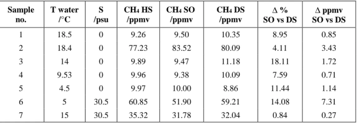
3.2 Comparison with Discrete Measurements

In order to prove the reliability of the extraction technique, a blind inter-comparison

with standard headspace equilibration technique followed by GC analysis was

performed. Seven independent measurements were conducted at different experimental

conditions of temperature and salinity. The results are summarized in Table 1.

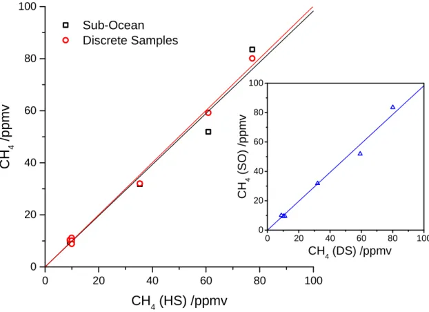
The concentrations measured by the Sub-Ocean spectrometer and by the GC from

the discrete samples was compared to the continuous measure obtained by the

spectrometer connected to the headspace. Slopes of 0.9830 ± 0.044 and 1.0016 ± 0.019

were obtained for SO/HS and DS/HS respectively (Figure 5). In the inset of Figure 5, the

results from SO and DS were directly compared and resulted in a slope of 0.9831 ±

0.031. The larger disagreement between the data corresponds to 18 % for sample No.3

(at 10 ppmv) and 7.3 ppmv for sample No.6 (60 ppmv) as reported in Table 1.

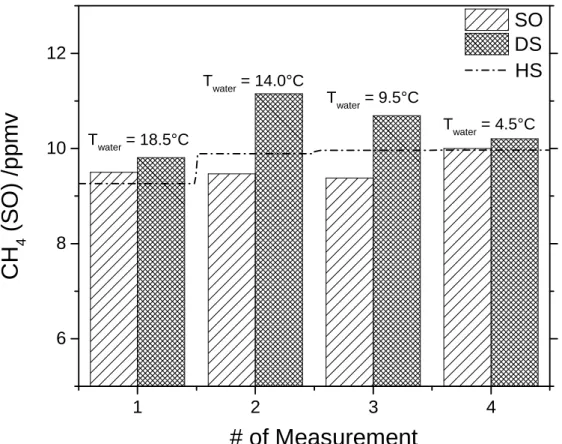
Four samples (1, 3, 4 and 5) were collected at different temperatures but similar

concentrations (10 ppmv) and used for studying the reproducibility of the measurement

with respect to the reference discrete sample method. Data are shown in Figure 6,

highlighting a comparable accuracy between the SO and DS measurement. Average

standard deviation for the four measurements at 10 ppmv with respect to the HS

measurement was 3.3% for the SO and 9.3% for the DS, while for the full set of the seven

measurements it was 6.6% for SO and 7.6% for DS.

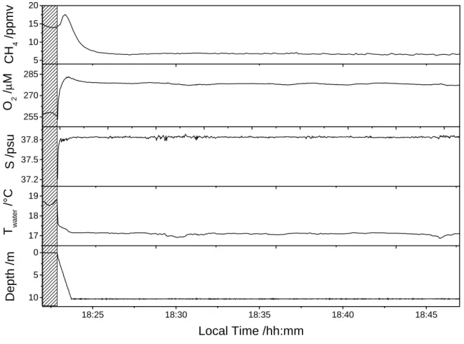
3.3 Field measurements

During the field campaign the probe was first tested by immersion at 10 m depth for

20 min, allowing for verification of the stability of the instrument as well as the full

functioning of the probe. This test was performed on July 12th _{at the position 43°6.20 N -}

5°56.73 E, close to the Toulon seaport. An example of the resulting data is shown in

16

after 50 s. The probe was left at the same depth for about 20 min, before being pulled up.

The standard deviation of the CH4 measurements over 20 min of immersion was 0.16

ppmv. It should be noted that the instrument was calibrated for subsea measurements,

therefore, the concentrations obtained in air (filled pattern area) are not correct, and are

reported here as a time reference. Afterward, the vessel was moved to an area off the

coast of Fréjus (position: 43°24.89 N - 7°00.61 E), where we performed vertical profiles

to greater depths. An example of the vertical profiles obtained is reported in Figure 8.

Here, 620 m of depth were reached in only 10 min.

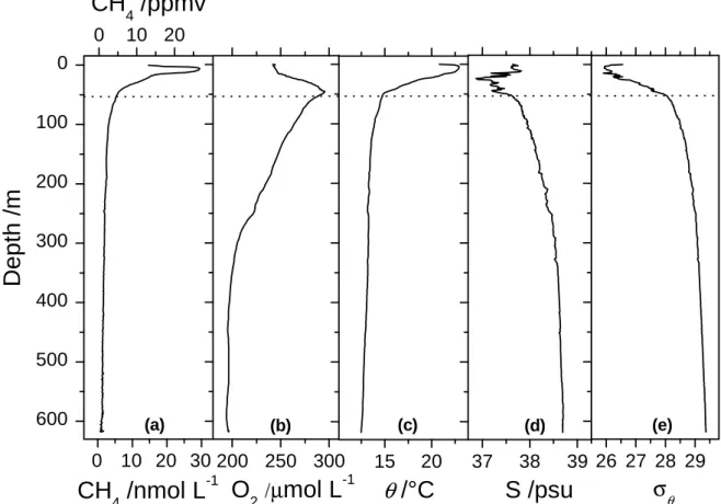
A temperature-salinity plot of this profile can be found in the SI-6. The potential

density anomaly increased from 26 to 28 kg m-3 _{from the surface down to 56 m (Figure}

8e), highlighting a strong stratification dominated by the temperature (Figure 8c).

Presence of fresh water above 56 m was observed through low salinity, but was

concealed in the top 25 m, where evaporation could be inferred through increased

salinity toward the surface. The dissolved oxygen peaked at 56 m, where the density

stratification weakened, and tapered off toward 350 m, but remained high down to the

end of the profile at 620 m.

The fast continuous measurements produced by the Sub-Ocean instrument

provide more details (600 data points) in the dissolved methane profile compared to

standard Niskin bottle sampling, where resolution is normally up to only 24 data points

per depth profile. Methane concentrations were 13 ppmv (15.4 nmol per liter of water)

at the surface, and they reached a maximum of 26.7 ppmv (30.2 nmol L-1_{) at 6 m water}

depth. Descending towards 620 m, CH4 concentrations decreased, approaching a

minimum of 0.6 ppmv (0.81 nmol L-1_{) close to the bottom. Unfortunately, during the}

campaign there were no facilities for collecting discrete samples for comparison.

17

indirect validation of the measurements can be done by comparing literature data of

background dissolved CH4 in seawater. 37

The relatively high methane levels observed at the surface (0 – 56 m),

supersaturated with respect to the atmosphere, are typical of most marine waters.38

This is the so-called “marine methane paradox” where methane (normally resulting

from the biological activity of strict anaerobes) is produced locally, while the

surrounding environment is rich in dissolved oxygen. This phenomena could be due to

aerobic bacterial degradation of phosphonate esters in dissolved organic matter as

revealed recently through incubation of seawater.7 _{No cytometry measurements or}

other biological and kinetic analyses were performed during our test campaign and

therefore, this hypothesis cannot be confirmed.

Another explanation for the CH4 profile could be that surface waters are mixed

with incoming freshwater. Water masses from the Rhone river plume, for instance, are

known to bear relatively large concentrations of dissolved methane, up to 1300 nmol L

-1_.34 _{A similarly CH4 enriched water source, for instance from the Var river, would also}

bear a minimum salinety signature. Such a signal appeared in our data set above 56 m,

(e.g. S = 36.9 at 24 m) but is located deeper than the methane maximum, which discards

the hypothesis of a freshwater anomaly to explain the methane one.

Comments and Recommendations

As shown in this initial work, the Sub-Ocean instrument opens new perspectives

for continuous monitoring of dissolved methane (and possibly other dissolved gases) in

sea- or lake waters. Its major advantages, compared with other instruments and

sampling methods include (1) short response times (τ90 = 30 s), (2) continuous in situ

18

laboratory analyses, (3) measurements that are immune to the presence of water vapor

or to interferences by other species present in the gas mixture, (4) high sensitivity of the

measurements (± 25 ppbv in air, translating into ± 0.03 nmol L-1 _{at 20°C and 38 psu of}

salinity in water) obtained with the highly sensitive OFCEAS optical spectrometer

embedded in the probe, allowing to measure anomalies in background concentrations,

(5) a large dynamical range, covering five orders of magnitude in CH4 concentrations.

Drawbacks of this approach are that (1) the measurement accuracy depends on the

stability of the extraction system (and particularly on the water flow through the

membrane) (2) enrichment factor (meff) will depends on the main components of the

dissolve gas and particular calibrations are required for environments where nitrogen

and oxygen are no longer the most abundant gas species.

This type of instrument could be employed for several applications such as studying

the stability of methane hydrates in the seafloor, monitoring biological activity in

seawater and lakes, checking leaks of natural gas pipes in deep water and pipelines

inspection. The telemetry feature, available by powering the sensor using a battery,

could provide real-time data at the surface via an electromechanical cable. This would

allow quantification of the evolution of dissolved gas in real-time from the ship, enabling

the design of more optimal ship-based sampling tracks. Here, we report the

measurement of dissolved methane, but this type of optical spectrometer also allows to

probe other target molecules such as CO2, N2O, and small hydrocarbons (C2 and C3), or

accessing to isotopic signatures of dissolved species such as δ13_{C and} δ_{D of CH4,} δ13_{C of}

CO2or directly the isotopic signature of the water mass (δD and δ18O). Further effort will

be made to miniaturize the device as well as to reduce the power consumption (50 W at

the moment with respect to 15-20 W for a commercial instrument) in order to allow

19

References

(1) Gentz, T.; Damm, E.; Schneider von Deimling, J.; Mau, S.; McGinnis, D. F.; Schlüter, M.

A water column study of methane around gas flares located at the West Spitsbergen

continental margin. Cont. Shelf Res. 2014, 72, 107–118.

(2) Ruppel, C. D.; Kessler, J. D. The interaction of climate change and methane hydrates.

Rev. Geophys. 2017, 55, 126–168.

(3) Bollmann, M.; Bosch, T.; Colijn, F.; Ebinghaus, R.; Froese, R.; Güssow, K.; Khalilian,

S.; Krastel, S.; Körtzinger, A.; Langenbuch, M.; et al. World Ocean Review, Living with

the oceans – A report on the state of the world’s oceans; 2010; Vol. WOR 1.

(4) Grossart, H.; Frindte, K.; Dziallas, C.; Eckert, W.; Tang, K. W. Microbial methane

production in oxygenated water column of an oligotrophic lake. PNAS 2011, 6 (49),

19657–19661.

(5) Damm, E.; Helmke, E.; Thoms, S.; Schauer, U.; Nothig, E.; Bakker, K.; Kiene, R. P.

Methane production in aerobic oligotrophic surface water in the central Arctic

Ocean. Biogeosciences 2010, 7, 1099–1108.

(6) Karl, D. M.; Beversdorf, L.; Bjorkman, K. M.; Church, M. J.; Martinez, A.; Delong, E. F.

Aerobic production of methane in the sea. Nat. Geosci. 2008, 1 (7), 473–478.

(7) Repeta, D. J.; Ferrón, S.; Sosa, O. A.; Johnson, C. G.; Repeta, L. D.; Acker, M.; DeLong,

E. F.; Karl, D. M. Marine methane paradox explained by bacterial degradation of

dissolved organic matter. Nat. Geosci. 2016, 9 (12), 884–887.

(8) Dohan, K.; Maximenko, N. Monitoring ocean currents with satellite sensors.

Oceanography 2010, 23 (4), 94–103.

(9) Gentemann, C. L.; Meissner, T.; Wentz, F. J. Accuracy of Satellite Sea Surface

Temperatures at 7 and 11 GHz. IEEE Trans. Geosci. Remote Sens. 2010, 48 (3), 1009–

20

(10) Abraham, J. P.; Baringer, M.; Bindoff, N. L.; Boyer, T.; Cheng, L. J.; Church, J. A.;

Conroy, J. L.; Domingues, C. M.; Fasullo, J. T.; Gilson, J.; et al. A review of global ocean

temperature observations: implications for ocean heat content estimates and

climate change. Rev. Geophys. 2013, 51, 450–483.

(11) Schlüter, M.; Linke, P.; Suess, E. Geochemistry of a sealed deep-sea borehole on the

Cascadia Margin. Mar. Geol. 1998, 148 (1–2), 9–20.

(12) Boulart, C.; Connelly, D. P.; Mowlem, M. C. Sensors and technologies for in situ

dissolved methane measurements and their evaluation using Technology

Readiness Levels. TrAC - Trends Anal. Chem. 2010, 29 (2), 186–195.

(13) Chua, E. J.; Savidge, W.; Short, R. T.; Cardenas-valencia, A. M.; Fulweiler, R. W. A

Review of the Emerging Field of Underwater Mass Spectrometry. Front. Mar. Sci.

2016, 3 (209).

(14) Newman, K. R.; Cormier, M.; Weissel, J. K.; Driscoll, N. W.; Kastner, M.; Solomon, E.

A.; Robertson, G.; Hill, J. C.; Singh, H.; Camilli, R.; et al. Active methane venting

observed at giant pockmarks along the U . S . mid-Atlantic shelf break. Earth Planet.

Sci. Lett. 2008, 267, 341–352.

(15) Wankel, S. D.; Huang, Y.-W.; Gupta, M.; Provencal, R.; Leen, J. B.; Fahrland, A.;

Vidoudez, C.; Girguis, P. R. Characterizing the distribution of methane sources and

cycling in the deep sea via in situ stable isotope analysis. Environ. Sci. Technol. 2013,

47 (3), 1478–1486.

(16) Michel, A. P. M.; Wankel, S. D.; Kapit, J.; Sandwith, Z.; Girguis, P. R. In situ carbon

isotopic exploration of an active submarine volcano. Deep. Res. Part II 2017.

(17) Faïn, X.; Chappellaz, J.; Rhodes, R. H.; Stowasser, C.; Blunier, T.; McConnell, J. R.;

Brook, E. J.; Preunkert, S.; Legrand, M.; Debois, T.; et al. High resolution

21

evidence for in situ production. Clim. Past 2014, 10 (3), 987–1000.

(18) Grilli, R.; Marrocco, N.; Desbois, T.; Guillerm, C.; Triest, J.; Kerstel, E.; Romanini, D.

Invited Article : SUBGLACIOR : An optical analyzer embedded in an Antarctic ice

probe for exploring the past climate. Rev. Sci. Instrum. 2014, 85 (111301), 1–8.

(19) Morville, J.; Kassi, S.; Chenevier, M.; Romanini, D. Fast, low-noise, mode-by-mode,

cavity-enhanced absorption spectroscopy by diode-laser self-locking. Appl. Phys. B

2005, 80 (8), 1027–1038.

(20) Morville, J.; Romanini, D.; Chenevier, M. WO03031949, (Université J. Fourier,

Grenoble FRANCE, 2003). WO03031949, 2003.

(21) Morville, J.; Romanini, D.; Kerstel, E. Cavity Enhanced Absorption Spectroscopy with

Optical Feedback. In Cavity-Enhanced Spectroscopy and Sensing; Gagliardi, G., Loock,

H.-P., Eds.; Springer Berlin Heidelberg, 2014; pp 163–209.

(22) Triest, J.; Chappellaz, J.; Grilli, R. Patent 08276-01: System for fast and in-situ

sampling of dissolved gases in the ocean (CNRS, Grenoble FRANCE, 2017). 8276–1.

(23) Chappellaz, J.; Alemany, O.; Romanini, D.; Kerstel, E. The IPICS « oldest ice »

challenge : a new technology to qualify potential sites. Ice Snow 2012, 4, 57–64.

(24) Fischer, H.; Severinghaus, J.; Brook, E.; Wolff, E.; Albert, M.; Alemany, O.; Arthern, R.;

Bentley, C.; Blankenship, D.; Chappellaz, J.; et al. Where to find 1.5 million yr old ice

for the IPICS “Oldest-Ice” ice core. Clim. Past 2013, 9 (6), 2489–2505.

(25) Lin, D.; Ding, Z.; Liu, L.; Ma, R. Gas Permeation through Polydimethylsiloxane

Membranes: Comparison of Three Model Combinations. Chem. Eng. Technol. 2012,

35 (10), 1833–1841.

(26) Robb, W. L. Thin silicon membranes. Their permeation properties and some

applications. Ann. N. Y. Acad. Sci. 1968, 146, 119–137.

22

Tech. Conf. Glob. Adv. Mater. Process Eng. 2006, 72–75.

(28) Merkel, T. C.; Bondar, V. I.; Nagai, K.; Freeman, B. D.; Pinnau, I. Gas sorption,

diffusion, and permeation in poly(dimethylsiloxane). J. Polym. Sci. Part B Polym.

Phys. 2000, 38 (3), 415–434.

(29) Mavroudi, M.; Kaldis, S. P.; Sakellaropoulos, G. P. A study of mass transfer resistance

in membrane gas-liquid contacting processes. J. Memb. Sci. 2006, 272 (1–2), 103–

115.

(30) Atchariyawut, S.; Feng, C.; Wang, R.; Jiraratananon, R.; Liang, D. T. Effect of

membrane structure on mass-transfer in the membrane gas-liquid contacting

process using microporous PVDF hollow fibers. J. Memb. Sci. 2006, 285 (1–2), 272–

281.

(31) Gonzalez-valencia, R.; Magana-rodriguez, F.; Gerardo-nieto, O.; Sepulveda-jauregui,

A.; Martinez-cruz, K.; Walter-anthony, K.; Baer, D.; Thalasso, F. In Situ Measurement

of Dissolved Methane and Carbon Dioxide in Freshwater Ecosystems by Off-Axis

Integrated Cavity Output Spectroscopy. Environ. Sci. Technol. 2014, 48, 11421–

11428.

(32) Schlüter, M.; Gentz, T. Application of Membrane Inlet Mass Spectrometry for Online

and In Situ Analysis of Methane in Aquatic Environments. J. Am. Soc. Mass Spectrom.

2008, 19 (10), 1395–1402.

(33) Schmidt, M.; Linke, P.; Esser, D. Recent Development in IR Sensor Technology for

Monitoring Subsea Methane Discharge. Mar. Technol. Soc. J. 2013, 47 (3), 27–36.

(34) Marty, D.; Bonin, P.; Michotey, V.; Bianchi, M. Bacterial biogas production in coastal

systems affected by freshwater inputs. Cont. Shelf Res. 2001, 21, 2105–2115.

(35) García-garcía, A.; Orange, D.; Lorenson, T.; Radakovitch, O.; Tesi, T.; Miserocchi, S.;

23 Gulf of Lions. Mar. Geol. 2006, 234, 215–231.

(36) Wiesenburg, D. A.; Guinasso, N. L. Equilibrium solubilities of methane, carbon

monoxide, and hydrogen in water and sea water. J. Chem. Eng. Data 1979, 24 (4),

356–360.

(37) Bates, T. S.; Kelly, K. C.; Johnson, J. E.; Gammon, R. H. A reevaluation of the open

ocean source of methane to the atmosphere. J. Geophys. Res. 1996, 101 (D3), 6953–

6961.

(38) Reeburgh, W. S. Oceanic Methane Biogeochemistry. Chem. Rev. 2007, 107, 486–513.

(39) Fofonoff, N. P.; Millard Jr., R. C. Algorithms for computation of fundamental

properties of seawater. Unesco Tech. Pap. Mar. Sci. 1983, 44, 53.

Acknowledgements

The research leading to these results has received funding from the European

Community’s Seventh Framework Programmes ERC-2011-AdG under grant agreement

n° 291062 (ERC ICE&LASERS), as well as ERC-2015-PoC under grant agreement no.

713619 (ERC OCEAN-IDs). This study is also a part of CAGE (Centre for Arctic Gas

Hydrate, Environment and Climate), Norwegian Research Council grant no. 223259).

The Téthys II ship time for the probe deployment in the Mediterranean Sea was

provided by the Commission Nationale de la Flotte Côtière of CNRS-INSU. We deeply

thank the captain of Téthys II Dany Deneuve and his crew, as well as the personnel of

DT-INSU and IFREMER at La Seyne sur Mer, for their help in setting up and deploying

the probe.

We acknowledge the SATT Linksium of Grenoble, France, and the Service Partenariat &

24

evaluate the valorisation potential of the Sub-Ocean instrument. We thank Dominique

Lefevre, Christian Tamburini at MIO-Marseille and Thierry Penduff at IGE-Grenoble for

25

Figures

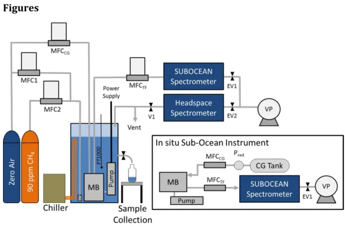
Figure 1. Experimental setup for laboratory tests. Two mass flow controllers (MFC1 and MFC2) have been employed to bubble different mixtures of CH4 in air into the water

sample via a diffuser place in the liquid solution. The membrane block (MB) and the water pump are immersed into the water sample, stabilized in temperature using an external chiller unit. The dry side of the membrane is continuously flushed with a small (1 to 6 sccm) dry gas flow supplied by the MFCCG, and the mixture (carrier gas plus

extracted gas) is sent to the Sub-Ocean spectrometer. The total flow is measured by a fourth mass flow controller MFCTF. A portion of the headspace CH4 concentration is

monitored using a second optical spectrometer based on the same absorption

spectroscopy technique (OFCEAS), while the overflow is sent to a vent. The exhausts of the analyzers are connected to two electronic valves (EV1 and EV2) and to a vacuum pump (VP) to ensure pressure regulation in the measurements gas cells. The inset shows the schematic of the in situ spectrometer, where the carrier gas flow is ensured using a gas tank and a pressure reducer, Pred.

26

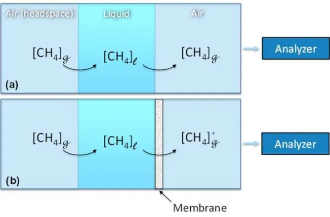
Figure 2. Schematic diagram showing the effect of a membrane for extracting dissolved

gas. (a) represents the (ideal) case without a membrane; here, the concentration of CH4 at

equilibrium found in the analyzed air will correspond to its concentration in the

headspace. (b) In the presence of a membrane, the measured CH4 concentration will be

affected by gas permeation through the membrane, resulting in a different measured

27

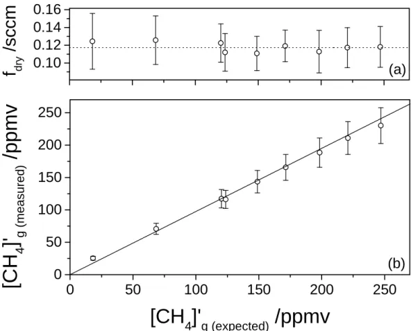
Figure 3. (a) Calculated flow of dry gas permeating through the membrane as a function

of the expected methane concentration. The average flow is 0.1173 ± 0.0017 sccm.(b)

CH4 concentrations measured downstream from the membrane by the Sub-Ocean

spectrometer are plotted against concentrations expected from the CH4 measured in the

headspace, after accounting for the methane enrichment due to its preferential

permeability through the silicon membrane, compared with molecular nitrogen and

oxygen. The measurement was performed with unsalted water at 18°C and 120 kPa of

pressure.

0

50

100

150

200

250

0

50

100

150

200

250

0.10

0.12

0.14

0.16

[C

H

]'

/

p

p

m

v

[CH

]'

/ppmv

(b)

f

/

s

c

c

m

(a)

28

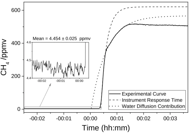
Figure 4. Typical response of the Sub-Ocean instrument when a water mass with high

concentration of dissolved CH4 is added to the analyzed water sample. The curve can be

fitted with a double-exponential growth function: a slow exponential (dotted line)

accounting for water mixing contribution, and a short one (dashed line) which

corresponds to the instrument response time. The τ90 of this second component corresponds to 30 s. A precision of ± 25 ppbv is obtained on the baseline (inset frame).

-00:02 -00:01 00:00 00:01 00:02 00:03 0 200 400 600 Experimental Curve

Instrument Response Time Water Diffusion Contribution

Mean = 4.454 ± 0.025 ppmv

C

H

/

p

p

m

v

Time (hh:mm)

29

Figure 5. Results from a laboratory inter-comparison between the Sub-Ocean probe (SO)

and the discrete sample method based on headspace equilibration followed by GC

analysis (DS). In the main plot is shown the comparison of both techniques with the

expected concentration measured by the headspace spectrometer (HS). In the inset plot

is shown the direct comparison between the two experimental methods.

0 20 40 60 80 100 0 20 40 60 80 100 Sub-Ocean Discrete Samples

C

H

/

p

p

m

v

CH

(HS) /ppmv

30

Figure 6. Reproducibility of Sub-Ocean (SO) and the discrete sample (DS) method at

similar concentrations and different water temperatures. The dashed line shows the

values expected from the headspace measurement during water equilibration and the

bars show the measured values for both methods. Averaged standard deviation

corresponds to 3.3 and 9.3 % for SO and DS methods, respectively.

1 2 3 4 6 8 10 12

C

H

(

S

O

)

/p

p

m

v

# of Measurement

SO

DS

HS

31

Figure 7. Static measurement at 10 m of depth for testing the Sub-Ocean system stability.

This test was done on July 12th_{, 2014 at the position 43°6.20 N - 5°56.73 E. In the plot is}

also reported the O2 concentration, temperature and salinity from a CTD that was

attached to the instrument. The standard deviation on CH4 concentration at 10 m of

depth over 20 min is 0.16 ppmv. 5 10 15 20 255 270 285 17 18 19 18:25 18:30 18:35 18:40 18:45 10 5 0 37.2 37.5 37.8 C H 4 / p p m v O 2 / µ M T w a te r / °C D e p th / m Local Time /hh:mm S / p s u

32

Figure 8. A continuous vertical profile of (a) CH4 (Sub-Ocean), (b) O2, (c) potential

temperature,

θ

σ

3h50 local time at the position 43°24.89 N - 7°00.61 E. Dissolved methane

concentrations have been converted in nmol per liter of water considering the solubility

of methane in water given by Wiesenburg, at 1 bar and at given temperature and salinity

according to CTD data. Potential density has been calculated according to ref 39_. 0 10 20 600 500 400 300 200 100 0 200 250 300 15 20 (e) (d) (c) (b)

CH

/ppmv

D

e

p

th

/

m

O

/µ

mol L

θ

/°C

S /psu

CH

/nmol L

σ

33

Tables

Table 1. Summary of the inter-comparison results. HS = headspace, SO = Sub-Ocean, DS = discrete samples.

Sample no. T water /°C S /psu CH4 HS /ppmv CH4 SO /ppmv CH4 DS /ppmv ∆ % SO vs DS ∆ ppmv SO vs DS 1 18.5 0 9.26 9.50 10.35 8.95 0.85 2 18.4 0 77.23 83.52 80.09 4.11 3.43 3 14 0 9.89 9.47 11.18 18.11 1.72 4 9.53 0 9.96 9.38 10.09 7.59 0.71 5 4.5 0 9.97 10.00 8.86 11.44 1.14 6 5 30.5 60.85 51.90 59.21 14.08 7.31 7 15 30.5 35.32 31.78 32.04 0.84 0.27