HAL Id: hal-03005989
https://hal.archives-ouvertes.fr/hal-03005989
Submitted on 5 Dec 2020
HAL is a multi-disciplinary open access
archive for the deposit and dissemination of sci-entific research documents, whether they are pub-lished or not. The documents may come from teaching and research institutions in France or abroad, or from public or private research centers.
L’archive ouverte pluridisciplinaire HAL, est destinée au dépôt et à la diffusion de documents scientifiques de niveau recherche, publiés ou non, émanant des établissements d’enseignement et de recherche français ou étrangers, des laboratoires publics ou privés.
A simulation method to infer tree allometry and forest
structure from airborne laser scanning and forest
inventories
Fabian Jörg Fischer, Fabian Fischer, Nicolas Labrière, Grégoire Vincent,
Bruno Hérault, Alfonso Alonso, Hervé Memiaghe, Pulchérie Bissiengou, David
Kenfack, Sassan Saatchi, et al.
To cite this version:
Fabian Jörg Fischer, Fabian Fischer, Nicolas Labrière, Grégoire Vincent, Bruno Hérault, et al.. A simu-lation method to infer tree allometry and forest structure from airborne laser scanning and forest inven-tories. Remote Sensing of Environment, Elsevier, 2020, 251, pp.112056. �10.1016/j.rse.2020.112056�. �hal-03005989�
A simulation method to infer tree allometry and
1forest structure from airborne laser scanning
2and forest inventories
3Fabian Jörg Fischera, *, Nicolas Labrièrea, Grégoire Vincentb, Bruno Héraultc,d,
4
Alfonso Alonsoe, Hervé Memiaghef, Pulchérie Bissiengoug, David Kenfackh, Sassan
5 Saatchii, and Jérôme Chavea 6 a Laboratoire Évolution et Diversité Biologique, UMR 5174 (CNRS/IRD/UPS), 118 7 Route de Narbonne, 31062 Toulouse Cedex 9, France 8 b AMAP, Univ Montpellier, IRD, CIRAD, CNRS, INRAE, Montpellier, France 9 c Cirad, Univ Montpellier, UR Forests & Societies, F-34000 Montpellier, France. 10 d INPHB, Institut National Polytechnique Félix Houphouët-Boigny, Yamoussoukro, 11 Ivory Coast 12 e Center for Conservation and Sustainability, Smithsonian Conservation Biology 13 Institute, 1100 Jefferson Drive SW, Suite 3123, Washington DC 20560-0705, USA 14 f Institut de Recherche en Écologie Tropicale (IRET), Centre National de la Recherche 15 Scientifique et Technologique (CENAREST), B.P. 13354, Libreville, Gabon 16 g Institut de Pharmacopée et de Médecine Traditionnelles (IPHAMETRA)/Herbier 17 National du Gabon, Centre National de la Recherche Scientifique et Technologique 18 (CENAREST), B.P. 1165, Libreville, Gabon 19 h Center for Tropical Forest Science -Forest Global Earth Observatory, Smithsonian 20 Tropical Research Institute, West Loading Dock, 10th and Constitution Ave NW, 21 Washington DC 20560, USA 22
i Jet Propulsion Laboratory, California Institute of Technology, 4800 Oak Grove Drive, 23 Pasadena, CA 91109, USA 24 25 * Correspondence: [email protected] 26 Keywords: vegetation structure; tropical forest; individual-based modeling; airborne 27 lidar; approximate bayesian computation; allometry; biomass; canopy space filling 28 29
Abstract 30 Tropical forests are characterized by large carbon stocks and high biodiversity, but they 31 are increasingly threatened by human activities. Since structure strongly influences the 32 functioning and resilience of forest communities and ecosystems, it is important to 33 quantify it at fine spatial scales. 34 Here, we propose a new simulation-based approach, the "Canopy Constructor", with 35 which we quantified forest structure and biomass at two tropical forest sites, one in 36 French Guiana, the other in Gabon. In a first step, the Canopy Constructor combines field 37 inventories and airborne lidar scans to create virtual 3D representations of forest 38 canopies that best fit the data. From those, it infers the forests' structure, including 39 crown packing densities and allometric scaling relationships between tree dimensions. 40 In a second step, the results of the first step are extrapolated to create virtual tree 41 inventories over the whole lidar-scanned area. 42 43 Across the French Guiana and Gabon plots, we reconstructed empirical canopies with a 44 mean absolute error of 3.98m [95% credibility interval: 3.02, 4.98], or 14.4%, and a 45 small upwards bias of 0.66m [-0.41, 1.8], or 2.7%. Height-stem diameter allometries 46 were inferred with more precision than crown-stem diameter allometries, with 47 generally larger heights at the Amazonian than the African site, but similar crown-stem 48 diameter allometries. Plot-based aboveground biomass was inferred to be larger in 49
French Guiana with 400.8 t ha-1 [366.2 – 437.9], compared to 302.2 t ha-1 in Gabon
50
[267.8 – 336.8] and decreased to 299.8 t ha-1 [275.9 – 333.9] and 251.8 t ha-1 [206.7 –
51
291.7] at the landscape scale, respectively. Predictive accuracy of the extrapolation 52
procedure had an RMSE of 53.7 t ha-1 (14.9% ) at the 1 ha scale and 87.6 t ha-1 (24.2%) at 53
the 0.25 ha scale, with a bias of -17.1 t ha-1 (-4.7%). This accuracy was similar to 54 regression-based approaches, but the Canopy Constructor improved the representation 55 of natural heterogeneity considerably, with its range of biomass estimates larger by 56 54% than regression-based estimates. 57 58 The Canopy Constructor is a comprehensive inference procedure that provides fine-59 scale and individual-based reconstructions even in dense tropical forests. It may thus 60 prove vital in the assessment and monitoring of those forests, and has the potential for a 61 wider applicability, for example in the exploration of ecological and physiological 62 relationships in space or the initialisation and calibration of forest growth models. 63
1. Introduction 64 Tropical forests store more than half of terrestrial living biomass (Pan et al., 2011) and 65 shelter a disproportionate share of terrestrial biodiversity. Yet they are increasingly 66 threatened by human activities, from agricultural encroachment and fragmentation to 67 global climate change (Lewis et al., 2015). Tropical forests thus play a pivotal role in 68 carbon mitigation and conservation strategies such as natural regeneration and the 69 avoidance of deforestation (Chazdon et al., 2016; Grassi et al., 2017). To prioritize such 70 strategies and assess their efficacy, methods are needed that accurately quantify forest 71 structure, i.e. the vertical and horizontal arrangement of tree stems and crowns. 72 Forest structure shapes ecosystem functioning (Shugart et al., 2010), wood 73 quality (Van Leeuwen et al., 2011), microclimates and habitats (Davis et al., 2019), and 74 the resilience and resistance of ecosystems to disturbances (DeRose and Long, 2014; 75 Seidl et al., 2014; Tanskanen et al., 2005). Forest structure also varies across climates 76 (Pan et al., 2013) and across successional states and environmental conditions (Lutz et 77 al., 2013). Approaches to quantify forest structure should therefore be able to account 78 for local heterogeneities and be applicable over large areas (R. Fischer et al., 2019). 79 Field-based inventories provide detailed descriptions of diameter distributions 80 across time and space and form the bedrock of research in forest ecology. However, the 81 mapping, measuring and identification of trees is typically limited to a few hectares. 82 Furthermore, it is usually difficult to obtain reliable measurements of tree height and 83 other crown dimensions from the ground (Sullivan et al., 2018). As a result, it has long 84 been a challenge to correctly describe the three-dimensional stratification of forests 85 (Oldeman, 1974). 86
Much has changed, however, with the advent of laser scanning and its ability to 87 obtain data in three dimensions (Atkins et al., 2018; Disney, 2019). At regional scales, 88 airborne laser scanning (ALS), i.e. aircraft-mounted laser scanning devices, are now 89 commonly used to survey forest stratification over thousands of hectares. The data can 90 be used to infer canopy height and leaf density at sub-meter resolution (Riaño et al., 91 2004; Rosette et al., 2008; Vincent et al., 2017), with diverse purposes, from estimating 92 carbon stocks (Asner and Mascaro, 2014) to mapping animal habitats (Goetz et al., 93 2010). In some situations, even individual tree dimensions – especially tree height, 94 crown area and depth – can be deduced by segmenting dense ALS point clouds into 95 individual plants and their components (Aubry-Kientz et al., 2019; Ferraz et al., 2016; 96 Hyyppä and Inkinen, 1999; Morsdorf et al., 2004). In particular for emergent and more 97 loosely spaced trees, full crowns are often visible in ALS datasets and can be monitored 98 from above (Levick and Asner, 2013; Meyer et al., 2018; Stovall et al., 2019). While this 99 technique has been well-researched in temperate and boreal forests, its implementation 100 is more difficult in the multistoried forests typically found in the tropics. In the latter 101 case, many trees are overtopped and difficult to delineate, so a large part of the 102 information on individual tree size is inaccessible. Furthermore, even when tree crowns 103 have been isolated, the matching of crowns to ground-measured diameters is made 104 difficult by asymmetries in tree growth and uncertainties in geo-positioning. 105 Here we propose an alternative, simulation-based strategy to infer forest 106 structure. It relies on a combination of ALS data and field inventories to first reconstruct 107 forests in 3D on local field plots, and then uses local summary statistics to create virtual 108 tree inventories over the whole ALS-extent. We call our method the "Canopy 109 Constructor". It is inspired by the fusion of forest simulators with lidar data (Fassnacht 110 et al., 2018; F. J. Fischer et al., 2019; Hurtt et al., 2004; Knapp et al., 2018; Shugart et al., 111
2015), space-filling algorithms (Bohn and Huth, 2017; Farrior et al., 2016; Taubert et al., 112 2015) and the use of synthetic forests to link lidar and ground inventories (Palace et al., 113 2015; Spriggs et al., 2015). The Canopy Constructor brings these approaches together to 114 provide a comprehensive picture of forest canopies in space, with applications in 115 biomass mapping, the study of remote sensing techniques and the initialization or 116 calibration of forest growth models (F. J. Fischer et al., 2019). 117 To implement it, we used the assumptions of the spatially explicit and individual-118 based forest growth model TROLL (Maréchaux and Chave 2017) and notions from 119 allometric scaling theories, i.e. that tree dimensions can be predicted through allometric 120 relationships (Niklas 2007) and that space-filling concepts translate between the 121 properties of individual trees and those of the whole stand (Niklas et al., 2003; West et 122 al., 2009). Unlike general theories of allometric scaling, however, the Canopy 123 Constructor seeks to infer realized scaling relationships from local plot data, and then 124 uses these to predict tree positions and dimensions in space. 125 Here, we describe the Canopy Constructor algorithm, and apply it at two tropical 126 rain forest sites, one in French Guiana (Chave et al., 2008a), one in Gabon (Memiaghe et 127 al., 2016), to infer the allometric relationships between trunk diameter and crown 128 dimensions, and to create virtual tree inventories across several thousands of hectares, 129 from which fine-scale above-ground biomass maps can be deduced. Specifically, we 130 asked the following questions: (i) How well can we reproduce 3D scenes of tropical 131 forests from relatively simple principles, (ii) Are tree inventories and ALS data sufficient 132 to infer allometric scaling relationships between tree dimensions, and how do these 133 relationships differ between sites? (iii) What is the biomass density at both sites and 134 how is it distributed across the landscape? (iv) How accurate is the Canopy Constructor 135 approach in extrapolation and does it have an advantage over conventional biomass 136
mapping methods? We evaluated the Canopy Constructor's predictions through 137 independent data and cross-validation, compared the accuracy against regression-based 138 approaches, and, for practical purposes, provide an assessment of its accuracy with a 139 reduced set of simulations. 140
2. Materials and Methods 141 2.1 Study sites 142 To answer our research questions, we selected two tropical sites, one in French Guiana, 143 and one in Gabon. The two sites were chosen based on their location in the Earth's two 144 largest tropical forest biomes, with high biomass and biodiversity, which makes it a 145 challenge to correctly estimate their structure. Furthermore, their biomass has been 146 recently quantified, so we had empirical data sets and estimates at hand to compare our 147 approach with (Labriere et al., 2018). Throughout, we refer to them as study sites, while 148 tree inventories are referred to as plots. 149 The French Guiana site is the Nouragues Ecological Research Station (4.06°N, 150 52.68°W). The site is characterised by a lowland tropical rainforest (except for a granitic 151 outcrop at 430m asl), ca. 2900 mm yr-1 rainfall, a 3-month dry season in September-152 November, and a shorter one in March. Its forest forms part of the Guiana Shield, at the 153 northeastern tip of Amazonia, a region with high tree wood densities and biomass, and a 154 large fraction of legume species (ter Steege et al., 2006). Tree inventories have been 155 carried out since 1992, including a 10-ha plot called "Grand Plateau" and a 12-ha plot 156 called "Petit Plateau" (Chave et al., 2008b). Trees with diameters ≥ 10 cm at 1.30m 157 above the ground (diameter at breast height, dbh) or above deformities and buttresses 158 are mapped, tagged and identified at species level when possible. The two plots differ in 159 their disturbance regime and canopy structure (cf. Figure S1 for their canopy height 160 models), but a typical hectare includes between 500 and 600 trees ≥ 10cm dbh and ≥ 161 150 tree species. Dominant species are Eschweilera coriacea, Quararibea duckei, Lecythis 162 persistens, Vouacapoua americana, Eperua falcata and the palm Astrocaryum sciophilum 163 (Poncy et al., 2001). Several ALS surveys have been conducted since 2008 (Réjou-164 Méchain et al., 2015), with a Riegl lidar (LMS-Q560) mounted on a fixed-wing aircraft. 165
We here used the 2012 tree inventory and ALS dataset which covers 2,400 ha at a pulse 166 density of ~12 per m2 (based on density of last returns) and an overall point density of 167 ~18 per m2 (all returns; Réjou-Méchain et al., 2015). 168 The second site, Rabi, is located in southwestern Gabon's Gamba Complex, 169 (1.92°S, 9.88°E). The site is characterized by annual rainfall of ca. 1970 mm yr-1 170 (Anderson-Teixeira et al., 2015a), and is covered with a lowland old-growth tropical rain 171 forest, with local human disturbances by oil operations and selective logging. A 25 ha 172 plot has been censused twice, including all trees ≥ 1 cm dbh, in 2010-2012 and 2016-173 2017 (Memiaghe et al., 2016), following the ForestGEO protocol (Condit, 1998). The plot 174
has an estimated 84 species ha-1 and 447 trees ≥ 10 cm dbh ha-1 (Memiaghe et al., 2016).
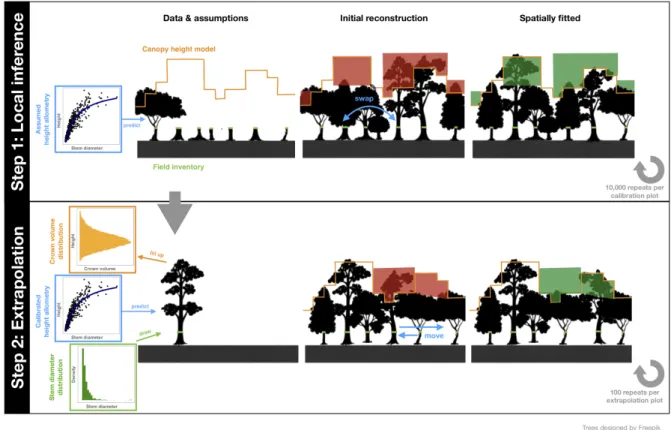
175 The legume family contributes a large fraction of species, trees and biomass, with four 176 species, Tetraberlinia moreliana, Tetraberlinia bifoliolata, Gilbertiodendron ogoouense, 177 and Amanoa strobilaceae, accounting for ca. 45% of canopy tree species (Engone Obiang 178 et al., 2019). An airborne lidar campaign over 900 ha was carried in 2015, using a 179 helicopter-based RIEGL VQ-480i, with pulse densities of ~2.5 per m2, and the plot is part 180 of the AfriSAR campaign (Fatoyinbo et al., 2017). 181 182 2.2 The Canopy Constructor algorithm 183 The Canopy Constructor algorithm consists of two steps. In a first step, the 3D-forest 184 structure is reconstructed over a local plot ("calibration plot"), relying on a tree 185 inventory, a co-registered ALS-scan and stand-average allometric relationships that 186 relate trunk diameter, tree height and crown radius. After an initial, random 187 reconstruction, tree properties are swapped until a high degree of similarity between 188 the empirical, ALS-derived canopy and the simulated canopy is achieved, but without 189 altering the underlying allometric structure. If allometric parameters are not known 190
empirically, they are inferred through Bayesian inversion where the routine is run with 191 a wide range of parameters (see e.g., Hartig et al., 2011). At the end this step, several 192 best-fit 3D scenes are obtained, representing the most likely structural configurations 193 and allometric scaling relationships on the calibration plot. 194 In a second step, the routine is extended to create a tree-by-tree reconstruction 195 over the whole extent of the airborne lidar scan. Trees are drawn from the local stem 196 diameter probability distribution and crowns are packed into the canopy until densities 197 match those of the calibration plot. In the following, we describe both steps in detail. 198 199 Figure 1: The two-step procedure of the Canopy Constructor algorithm. Step 1 uses tree inventory 200 data, and a canopy height model (CHM). To infer the position and size of each tree, the algorithm creates 201 an initial reconstruction drawing randomly dimensions from allometric relationships between tree 202 dimensions. In ill-fitting regions (red), deviations from the allometric means are swapped between trees 203 until a good spatial fit is obtained (green). Step 2 extrapolates the results of step 1 and creates virtual 204 inventories across thousands of hectares, following the same fitting algorithm as in step 1, but with fitted 205 trees drawn from a distribution (see main text for details). 206
The code was developed in C++ and is available online 207 (https://github.com/fischer-fjd/CanopyConstructor). Statistical analysis and 208 visualization were carried out in R (R Development Core Team, 2019) with the packages 209 data.table, raster, ggplot2, and viridis (Dowle and Srinivasan, 2018; Garnier, 2018; 210 Hijmans, 2016; Wickham, 2011) and their dependencies. 211 212 2.2.1 Forest structure inference and model calibration 213 The Canopy Constructor inputs tree diameters and locations from a forest inventory, 214 predicts tree heights and crown diameters from allometric scaling and fills up an initial 215 3D-canopy for the fitting procedure (resolution of 1m3), as in the TROLL model 216 (Maréchaux and Chave, 2017). To summarize canopy structure, we chose the canopy 217 height model (CHM), defined as the top-of-canopy height above ground for a given grid 218 cell (here at 1m2 resolution). For the tree-by-tree reconstruction, the minimal trunk 219 diameter size was set to 1 cm. Each surveyed tree was assigned to a grid with 1m2 cell 220 size. If several trees co-occured on the same cell, their positions were slightly jittered to 221 fill up adjacent cells. For multistemmed trees, a single effective stem dbh was retained, 222 equal to 𝑑𝑏ℎ!"" = 𝑑𝑏ℎ!! ! . For simplicity, we refer to 𝑑𝑏ℎ!"" as dbh. For tree 223
inventories with a higher cutoff than 1 cm (e.g. dbhcutoff = 10cm or 30cm), power-law and
224 exponential dbh-size distributions were assumed to fill up and randomly place trees < 225 dbhcutoff (Taubert et al., 2015, Farrior et al., 2018). 226 227 Allometric relationships 228 To predict canopy structure from the field-measured stems, the Canopy Constructor 229 assumes the following allometric models: 230
ℎ =ℎ𝑚𝑎𝑥 × 𝑑𝑏ℎ𝑎 !+ 𝑑𝑏ℎ × exp (𝜀!) ( 1 ) and 231 𝑐𝑟 = exp 𝑎!" + 𝜀!" ×𝑑𝑏ℎ!!" ( 2 ) In Equation (1), h is total tree height, dbh diameter at breast height, while hmax and ah 232 are Michaelis Menten coefficients interpreted as the asymptotic height that trees reach 233 at large trunk diameter values and the approximately linear slope of the increase of 234 height with diameter at small trunk diameters, respectively. In Equation (2), cr is the 235
tree's crown radius, and acr and bcr are the intercept and slope of a log-log regression, i.e.
236
a power law model. Equation (1) was chosen instead of a power model to better capture 237
the saturating relationships typically found in tropical rain forests (Cano et al., 2019). 238
The 𝜀! and 𝜀!" are the respective error terms – i.e. the natural variation in allometry –, 239 given by: 240 𝜀! ~ 𝑁(0, 𝜎!) ( 3 ) and 241 𝜀!" ~ 𝑁(0, 𝜎!") ( 4 ) The error terms generate a multiplicative error structure that accounts for the 242 heteroscedasticity in crown and height allometries (Molto et al., 2014). We assumed that 243
allometric variation did not depend on species identity, that 𝜀! and 𝜀!" were 244 independent, and that crown depth could be simply calculated as a proportion of h, as in 245 the TROLL model (Maréchaux and Chave, 2017). 246 To model crown shape more realistically, we defined the ratio 𝛾 between the 247 radius at the top of the crown and its base, with a linear slope linking both layers. 𝛾 248
varies between 0 and 1: if 𝛾 = 0, the tree crown is a cone, while if 𝛾 = 1, it is a cylinder 249
(as in Maréchaux & Chave, 2017). For the purposes of this study, we set 𝛾 to 0.8. This 250
resulted in an improvement in the convergence of the crown fitting algorithm compared 251 to simpler cylindrical shapes, better modelled the less clear-cut edges found empirically 252 and accounted for the fact that real tree crowns are smaller than their cylindrical 253 envelopes. 254 Based on the crown shape parameter as well as a particular realization of the six 255 allometric parameters (hmax, 𝑎!, 𝑎!", 𝑏!", 𝜀!, 𝜀!"), we created an initial 3D forest mockup, 256 with deviations from allometric means randomly assigned to trees. 257 258 Optimization algorithm 259 The Canopy Constructor then optimizes the spatial overlap of the simulated and the 260 ALS-derived CHMs by readjusting trees and their crowns in space. To this effect, we 261 looped repeatedly through all trees on the grid, in random order, and applied one of 262 three operations described below. The loop was stopped when improvements in canopy 263 structure were marginal (< 1% acceptance rates), usually achieved after 100-200 264 iterations. A similar algorithm was implemented in Taubert et al. (2015). 265 For the majority of field-measured trees, we picked pairs of trees and swapped 266
their respective values of 𝜀! (deviation in height) and 𝜀!" (deviation in crown radius). 267 We then recalculated the new dimensions of both trees and kept the change if it resulted 268 in an increase in the overall goodness of fit between the simulated and ALS-derived 269 CHM. To keep the overall variance structure, trees were binned into logarithmic dbh 270 classes and only swapped when they were in the same dbh class. This procedure rapidly 271 redistributed deviations from the allometric means across the population of trees so as 272 to improve spatial fits, but preserved the initial allometric structure. 273 We defined two exceptions. First, large tree crowns are crucial to obtain a good 274 canopy reconstruction, but only have limited opportunities to swap dimensions due to 275
their low numbers. Therefore, if there were less than 10 trees within a dbh bin across 276 the plot, we drew new tree sizes from equations (1) and (2). If the new draw resulted in 277 a better fit to empirical data, it was retained. To prevent bias in the allometric structure, 278 the expected crown radii and heights had to be preserved. We used a simple method, 279 allowing positive deviations from the mean only if the previous bin average deviated 280 negatively from the expected value, and vice versa. 281
Second, for trees with dbh < dbhcutoff, initial positions were chosen at random, so
282 we did not change the trees' dimensions, but instead relocated the entire tree, within a 283 radius dependent on its height (but at least 10 m). If the new location increased the 284 goodness of fit, the change was accepted. Few small trees were visible in the CHM, so 285 this procedure rarely modified the canopy, except in canopy gaps. 286 Plot boundaries bisect crown areas and may thus introduce errors in estimation 287 procedures (Mascaro et al., 2011). To prevent biased estimates, we calculated the crown 288 area outside the plot 𝐶𝐴!!"# and the total crown area 𝐶𝐴 ! for each tree i, summed both 289 across all n trees per plot and computed the ratio 𝑅 = !!!!!"!!"# !!! ! !!! . During the optimization 290 procedure, we forced R to remain approximately constant. If during the fitting process, R 291 exceeded its initial value, then the trial was accepted only if it lowered R, and vice versa. 292 We further observed that the Canopy Constructor could assign large crowns to 293 lower canopy layers that barely affected the CHM and fit small crowns on the tallest 294 trees to mimick natural heterogeneity, a phenomenon similar to oversegmentation in 295 tree delineation approaches. To prevent this, we circled through all trees within a 296
distance dist = CRtree + CRtreemax, for every newly fitted crown with CRtree, and rejected
297
crown fittings that resulted in tree configurations where a large tree with a small crown 298
pierced a small tree with a large crown. 299
300 Goodness-of-fit metrics 301 Each time a tree crown was updated, we tested whether this change increased the fit 302 with empirical values. To assess the goodness of the fit between virtual and empirical 303 CHMs, we used the mean of the absolute errors: 304 𝑀𝐴𝐸 =𝑠 1 !"!#$ 𝑐ℎ𝑚!"# 𝑠 − 𝑐ℎ𝑚!"# 𝑠 !!"!#$ !!! ( 5 )
where each s represents a 1m2 grid cell of forest, chmemp the empirical canopy height of
305
that grid cell, chmsim the simulated canopy height, derived from the highest non-empty 306
voxel, and stotal the total number of grid cells within the plot. MAE measures the
307 matching of local canopy height patterns and was used instead of a mean squared error, 308 because it is more robust with regard to outliers (Hill and Holland, 1977). 309 Since initial tests showed that the size of large trees would be underestimated by 310 shrinkage towards the mean from an optimization of MAE alone, we also used the 311 dissimilarity index of the canopy height distributions: 312 𝐷 = 1 2 d!"# ℎ − d!"# ℎ !!!!"# !!! ( 6 )
where h is a discrete height index (in m), and d!"# and d!"# are the densities of the 313 empirical and simulated height histograms across the surveyed area, i.e. total number of 314 canopy height occurrences, normalized by the number of 1m2 grid cells. The factor ½ 315 normalizes the metric to 1 and allows us to interpret it as a measure of distribution 316 overlap: the lower the dissimilarity, the higher the overlap. In the limit of D = 0, both 317 distributions are identical, in the limit of D = 1, there is no overlap at all. Formally, if OVL 318 is the distribution overlap, then D = 1 – OVL, with 𝑂𝑉𝐿 = !!"#!!! min 𝑑!"# ℎ , 𝑑!"# ℎ 319 (Inman and Bradley, 1989; Swain and Ballard, 1991). 320
We fitted the tree crowns using both metrics independently first, until a low 321 acceptance rate was achieved for each (< 1% for trees > 10cm dbh, typically reached 322 within 50 iterations for the MAE, and within 5 iterations for the dissimilarity). We then 323 used the difference between initial and final fits to normalize both metrics and 324 combined the normalized values to an overall error as follows: 325 𝛿 = 𝑀𝐴𝐸!"#$! + 𝐷 !"#$! ( 7 ) In a final number of iterations, we minimized 𝛿. The combined metric ensured that 326 crowns did not only fit spatially at local scales, encapsulated by a low MAE, but also 327 preserved the overall canopy height model distribution, as measured by D. 328 329 Inferring Allometric Parameters by Approximate Bayesian Computation 330 The optimization algorithm finds the best canopy reconstruction, given a set of 331 allometric parameters. However, allometric parameters are rarely known, so we used an 332 Approximate Bayesian Computation rejection scheme (Csilléry et al., 2010; Hartig et al., 333 2014; F. J. Fischer et al., 2019) to infer them. The prior probability distribution of the six 334
allometric parameters, (hmax, ah, acr, bcr) and (𝜎!, 𝜎!") was approximated by 10,000
335 random draws. We applied the Canopy Constructor to the allometric parameter 336 combinations, and retained only the best 1% of canopy reconstructions (Csilléry et al., 337 2010). The retained parameter values were used to generate a posterior probability 338 distribution over credible allometric parameterizations given the data. 339 We chose flat parameter priors by drawing from uniform distributions within 340 globally observed ranges of tree allometries (Jucker et al., 2017). Parameters were 341 drawn on logscales, except for the crown allometry intercept acr, drawn from a uniform 342 distribution on the back-transformed scale. A Latin hypercube scheme was employed to 343 minimize the computational burden, and correlation between allometric coefficients 344
was accounted for using an algorithm of the R package 'pse' (Chalom et al., 2013), 345 rewritten in C++ for speed. Covariance coefficients were taken from the Jucker et al. data 346 set (2017). Since crown depth did not influence canopy height – and thus did not 347 directly affect the fitting procedure –, it was fixed to 20% of tree height throughout the 348 procedure. 349 To assess goodness of fit, we again used the mean absolute error (MAE) and 350 dissimilarity D. But instead of normalizing by the within-simulation range, we 351 normalized by the range across all simulations and combined the metrics to 𝛿!"# = 352 𝑀𝐴𝐸!"#$%&!! + 𝐷 !"#$%&'! . 353 354 2.2.2 Model extrapolation 355 In step 2, the Canopy Constructor uses the local fit from step 1, extrapolates the trunk 356 diameter probability distribution and allometric scaling relationships across the whole 357 ALS-covered area and constructs virtual tree inventories from space-filling principles. 358 We implemented the same fitting procedure as before, but since the location and size of 359 stem diameters have to be inferred, now all trees are drawn from a distribution and 360 then relocated to create better spatial fits. 361 362 Space-filling principles 363 As a measure of space-filling, we used the crown packing density 𝜑 = !! !"# !𝑉!, where 364
Vmax is the maximally available volume within a section of the canopy, and Vi the volume
365 contribution of each tree to that section (Jucker et al., 2015; Taubert et al., 2015). The 366 crown packing density is the ratio of unit crown volume to unit canopy volume (m3 per 367 m3). It can be calculated for single voxels, subsets of voxels or for the entire canopy. 368
We defined the crown packing density at height h, with 0 ≤ ℎ ≤ ℎ!"#, and with 369 ℎ!"# top-of-canopy height, so that crown packing density was dependent on the 370 canopy's height. We then defined the following quantity: 𝝋 ℎ, ℎ!"# , the packing density 371 matrix, where columns represent top-of-canopy height ℎ!"# and rows represent within-372 canopy height layers h (cf. Figure S2, left panel). We set the size of height bins to 1 m, 373 and their numbers ran from 0 m to maximum canopy height. On a per-voxel basis, each 374 tree's volume contribution to a voxel could thus be either 0 or 1 m3, but due to the 375 idealized crown shapes assumed in the Canopy Constructor, crown overlaps were more 376 frequent than in real forest stands, resulting in local packing densities > 1 m3. 377 378 Inferring virtual inventories 379 To infer virtual tree inventories across the whole ALS-covered area, we divided the lidar 380 scene into grid cells, roughly equivalent in size to the local field inventories. We then 381 used the CHM of each grid cell, combined it with the packing density matrix 𝝋 obtained 382 from the 3D reconstructions of the local calibration plot and predicted crown volume 383 per height layer. This was achieved by calculating the ALS-derived canopy height 384 distribution for each grid cell, denoted 𝑐!"#, and formalized as a vector of top-of-canopy 385 height frequencies. Multiplying the ALS-derived canopy height vector with the packing 386
density matrix yielded the vector 𝑣!"# = 𝝋𝑐!"# (Figure S2). The quantity 𝑣!"# is an 387 estimate of total crown volume per height layer within the extrapolation cell. For grid 388 cells that reached canopy heights larger than the calibration plot from which the packing 389 density matrix was derived, 𝝋 was calculated by averaging over the five non-empty 390 layers just beneath the missing layer. 391 Once the maximum space filling was determined, trees were drawn until a virtual 392
forest with a crown volume distribution 𝑣!"#$%&' similar to 𝑣!"# was obtained. We drew 393
diameters from the calibration plot's probability distribution and used the previously 394
inferred allometric relationships to predict tree height and crown radius. After 395
randomly placing a tree on the grid, we updated 𝑣!"#$%&' and determined by how much
396 the new tree improved the fit with 𝑣!"#. To do so, we calculated the change in 𝑣!"## ℎ = 397 𝑣!"# ℎ − 𝑣!"#$%&' ℎ for every height layer h. If the crown volume in h had not yet 398 reached the reference value (𝑣!"## ℎ > 0), every added unit of crown volume improved 399 the fit and was counted positively. As soon as the crown volume in the layer reached or 400 exceeded the ALS-predicted volume (𝑣!"## ℎ ≤ 0), every added crown volume unit 401 penalized the fit and was thus discounted. We then summed units of crown volume over 402 all layers h, and we accepted the tree if the overall balance was positive. Otherwise, the 403 tree was rejected. Each drawing cycle comprised n draws, where n is the number of 404 potential tree locations (i.e. the m2 area) under consideration. When the rejection rate 405 reached 100% after a full cycle, we stopped the procedure. 406 After the initial distribution of trees in space was obtained, it was gradually 407 improved upon. This was done by displacing trees in relation to their height until an 408 optimal spatial fit was achieved, as described for step 1. Again, we found that 100-200 409 iterations were sufficient to reach low rejection rates (< 1%). To propagate uncertainty, 410 the procedure was carried out for each of the 100 posterior reconstruction of the ABC 411 approach from step 1, with all grid cells collated to produce final maps. 412 413 2.2.3 Application at the study sites 414 At Nouragues, we used the geographically separated Petit Plateau (12 ha) and Grand 415 Plateau (10 ha). Applying the inference step on each of them individually allowed for a 416 comparison with previous studies and an assessment of within-site heterogeneity. We 417 also split the 25-ha plot at Rabi into two subplots (10-ha and 15-ha, respectively). We 418
used plot sizes of ≥ 10ha because they minimized edge effects and kept a balance 419 between the computational burden of the procedure and the sample sizes needed to 420 swap random terms between crowns. On each subplot, we inferred forest structure (tree 421 dimensions, allometric parameters and crown packing densities). We then used the 422 larger plots at both sites (i.e. the 12 ha Petit Plateau and the 15 ha Rabi plot) to 423 extrapolate the virtual inventories across the whole landscape, subdivided into 400m x 424 400m grid cells (16 ha). Grid cells at the edges were discarded, and we created virtual 425 forest inventories over 2,016 ha at Nouragues and 832 ha at Rabi. 426 To create the CHMs, lidar data were classified via TerraScan and then post-427 processed with LAStools to obtain pit-free CHMs (Isenburg, 2018; Khosravipour et al., 428 2014). While the ALS data differed in point densities at the two sites (with considerably 429 lower densities at Rabi), the Canopy Constructor method was robust to such differences 430 because it was based on the CHM alone. Aboveground biomass (AGB) was estimated for 431 each tree (kg), using the formula 𝐴𝐺𝐵 = 0.0673 × 𝜌×𝑑𝑏ℎ!×ℎ !.!"# (Chave et al., 2014), 432 where ρ represents species-level wood density, obtained from a global database (Chave 433 et al., 2009; Zanne et al., 2009). For biomass mapping, tree biomass estimates were 434 aggreggated at 1 ha and 0.25 ha resolutions (t ha-1), a common grid size in biomass 435 mapping (Labrière et al., 2018; Réjou-Méchain et al., 2015). For consistency with 436 previous work, we computed AGB only for trees with dbh ≥ 10cm. Diameter 437 measurement errors usually have small effects on plot-scale estimates (Réjou-Méchain 438 et al., 2017), and since neither ρ nor error in the AGB equation directly affected the 439 Canopy Constructor algorithm, we did not propagate error in these quantities. 440 441 442 443
444 2.3 Evaluation 445 We assessed the accuracy of the Canopy Constructor's reconstructions (step 1) by 446 comparing the inferred allometric relationships between trunk diameters and tree 447 dimensions to allometric relationships derived from field measurements of tree height 448 and diameter. We computed the mean absolute and mean relative deviation (in %) 449 between height predictions. For biomass, we compared our predictions to previous 450 estimates of plot biomass for both sites and landscape-scale maps obtained with a 451 pooled regression model, all reported in Labriere et. al. (2018). 452 To more formally assess the extrapolation to landscape scale (step 2), we first 453 evaluated the consistency of the extrapolation model with the reference estimate, 454 derived from the field inventory and Canopy Constructor-calibrated allometries (step 1). 455 We did so by applying the extrapolation step to each plot itself and assessed the fit of the 456 extrapolation model. We quantified the accuracy and precision of biomass estimation 457 via four commonly reported metrics, namely R2 (squared Pearson's r), RMSE (root mean 458
squared error, t ha-1), MAE (mean absolute error, t ha-1) and MBE (mean bias of the
459
error, t ha-1). All metrics, except R2, were also computed relative to the reference AGB.
460 We then evaluated the sensitivity to plot characteristics through a cross-validation 461 procedure where we used the summary statistics from one plot per study site 462 (calibration plot) to extrapolate to the other plot at the study site (extrapolation plot), 463 and vice versa. As before, we quantified accuracy with respect to reference AGB 464 estimates through R2, RMSE, MAE and MBE. Finally, we also compared the reference and 465 predicted diameter distributions, both for the model fit and in cross-validation. 466 To evaluate the Canopy Constructor's utility for biomass estimates compared to 467 more conventional methods, we compared its accuracy to the accuracy of log-log 468
regression models of AGB vs. median canopy height (Labriere et al., 2018; Réjou-469 Méchain et al., 2015). We fitted log-log regression models against median canopy height, 470 again for each of the four plots at both 1 ha and 0.25 ha resolution and assessed both 471 model fit at the calibration plot and predictions between cross-validation plots. To 472 mirror the Canopy Constructor setup, we did not use any field-inferred height 473 allometries for the AGB estimates, but inferred height from a bioclimatic predictor 474 (Chave et al., 2014; Réjou-Méchain et al., 2017). Accuracy was reported with the same 475 metrics as above (R2, RMSE, MAE, MBE). 476 Throughout this study, we carried out a comprehensive Bayesian inference with 477 10,000 prior and 100 posterior simulations. This gave a good approximation of the 478 Canopy Constructor's posterior distributions, but, more importantly, also allowed us to 479 assess the method's sensitivity to simulation numbers. To this effect, we resampled 100 480 sets of 1,000 simulations from the 10,000 prior simulations, and 100 sets of 10 481 simulations from the 100 posterior simulations, and repeated both steps of the Canopy 482 Constructor to assess accuracy and precision in a computationally more efficient setting. 483
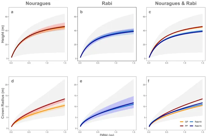
3. Results 484 3.1 Reconstructions of tropical forest canopies in 3D 485 Across all plots, the Canopy Constructor yielded good fits for the canopies with a final 486 error in mean canopy height of 0.66m [95% credibility interval: -0.41, 1.8] or 2.7% of 487 mean canopy height, and a mean absolute error of 3.98m [3.02, 4.98] or ~14.4% of 488 mean canopy height. Figure 2 visualizes the approach at the Petit Plateau plot for a 489 posterior simulation after 200 iterations of fitting. The initial draw (panel a) already 490 mirrored average properties of the empirical canopy, but not the spatial location of its 491 features (panel b). Swapping the deviations in allometries greatly improved the spatial 492 structure (panel c). 493 494 Figure 2: Example of canopy reconstruction at the Petit Plateau plot, Nouragues. Shown are the 495 initial canopy height model (CHM) where tree dimensions are randomly drawn from site-specific 496 allometries (a), the ALS-derived CHM (b), and the final reconstruction of the Canopy Constructor (c). 497 498 3.2 Allometric scaling relationships 499 Tree inventories and ALS data were sufficient to infer allometric relationships between 500 tree dimensions at both sites. Across all plots, we found substantial covariation between 501 allometric parameters (Table S1, and Figure S3, left panels), but height allometries had 502 lower uncertainties than crown radius allometries (Figure 3, Figure S3, Table 1). High 503 within-site similarity was found for height allometries at both Nouragues and Rabi 504 (Figure 3). Crown allometries, on the other hand, showed a divergence at Nouragues, 505 a 0 20 40 60 Height (m) b 100 m c
with larger crown radii predicted at Petit Plateau than at Grand Plateau. The sites were 506 clearly distinct in their height allometries, with generally taller trees at Nourages than at 507 Rabi, but not in their crown allometries. 508 509 510 Figure 3: Inferred allometries at Nouragues and Rabi (step 1). The panels show height allometries 511 (top row) and crown allometries (bottom row), as inferred by the Canopy Constructor, for Nouragues 512 (a,d), Rabi (b,e) and both sites combined (c,f). The grey background indicates the prior range. Mean and 513 75% highest density intervals are given for each plot separately, i.e. for Grand Plateau (orange) and Petit 514 Plateau (dark red) at Nouragues, and for the 10ha (light blue) and 15ha (dark blue) plot at Rabi. As 515 comparison, we have plotted empirical height allometries measured from in the field for both Grand 516 Plateau (dotted) and Petit Plateau (dashed) in the top panels, as well as a single ground-inferred allometry 517 at Rabi (dotted). Results for same inference procedure, but with a lower number of simulation runs, are 518 provided in Figure S8. 519 520 a 0 20 40 60 0.0 0.5 1.0 1.5 DBH (m) Hei g h t (m) Nouragues d 0 5 10 15 20 0.0 0.5 1.0 1.5 Cro w n Rad iu s (m) b 0 20 40 60 0.0 0.5 1.0 1.5 DBH (m) Hei g h t (m) Rabi e 0 5 10 15 20 0.0 0.5 1.0 1.5 DBH (m) Cro w n Rad iu s (m) c 0 20 40 60 0.0 0.5 1.0 1.5 DBH (m) Hei g h t (m)
Nouragues & Rabi
f 0 5 10 15 20 0.0 0.5 1.0 1.5 Cro w n Rad iu s (m) GP PP Rabi10 Rabi15
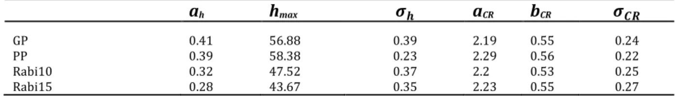
At both sites, parameter estimates were close to those previously obtained from 521 field measurements of tree height (cf. Figure 3, top row). At Nouragues, the Canopy 522 Constructor's height estimates were slightly lower than empirical ones at small 523 diameters and exceeded them at large diameters, but mirrored their qualitative 524 patterns, i.e. the larger heights predicted at Petit Plateau compared to Grand Plateau. 525 The difference to empirical height predictions never exceeded 1m (or 2%) at Petit 526 Plateau, versus 3.2 m (or 7.8%) at Grand Plateau. At Rabi, the pattern was inversed, with 527 lower predictions of tree height at large diameters than from empirical data, but 528 differences never exceeded 11% (Supplementary Figure S4). 529 Table 1: Inferred parameters. Mean of posterior distributions for allometric parameters at the two sites. 530 Plots are Grand Plateau (GP) and Petit Plateau (PP) at Nouragues, and the 10 ha and 15 ha rectangular 531
strips at Rabi (Rabi10 and Rabi15, respectively). ah and hmax are given in m, all other variables are unitless.
532 ah hmax 𝝈𝒉 aCR bCR 𝝈𝑪𝑹 GP 0.41 56.88 0.39 2.19 0.55 0.24 PP 0.39 58.38 0.23 2.29 0.56 0.22 Rabi10 0.32 47.52 0.37 2.2 0.53 0.25 Rabi15 0.28 43.67 0.35 2.23 0.55 0.27 533 534 3.3 Biomass mapping at landscape scale 535 Aboveground biomass was estimated to be 400.8 t ha-1 at the Nouragues plots [366.2 – 536 437.9] and 302.2 t ha-1 [267.8, 336.8] at Rabi. Within-site standard deviation at hectare 537
scale was 105.1 t ha-1 [86.5, 120.7] at Nouragues and 71.0 t ha-1 [60.5, 83.6] at Rabi. At
538 both sites, biomass density decreased at the landscape scale to an average of 299.8 t ha-1 539 [275.9, 333.9] and 251.8 t ha-1 [206.7, 291.7], respectively, but with considerable 540 heterogeneity (Figure 4, a and d). Map uncertainty was highest at vegetation edges and 541 low biomass areas, and generally higher at Rabi (median coefficient of variation of 542 ~0.24) than at Nouragues (~0.16, cf. also Figure 4, b and e). At both Nouragues and Rabi, 543
aboveground biomass reached similar extreme values, of over 1100 t ha-1 at the 0.25-ha 544 scale. 545 546 Figure 4: Aboveground biomass predictions for ALS campaign at Nouragues and Rabi (step 2). 547 Maps show the mean aboveground biomass values (t ha-1) predicted with the Canopy Constructor 548 approach across 2,016 ha at Nouragues (panel a) and 832 ha at Rabi (panel d), as well as the respective 549 coefficient of variation across 100 simulations (panels b and e, dimensionless). Also given are the overall 550 distributions of aboveground biomass (panels c and f, red distributions, in t ha-1) and previously obtained 551 estimates (panels c and f, yellow) from a pooled regression-model (Labrière et al. 2018). Clearly evident is 552 the shrinkage towards the mean in the regression-based approach, as opposed to much stronger variation 553 in the Canopy Constructor approach. Please note that the geographic extent of the maps has been rescaled 554 for visualization purposes. 555
Biomass estimates were close, but lower at both sites than previous estimates of 556 404.6 t ha-1 at the plot and 328.6 t ha-1 at landscape scale at Nouragues, and 314.6 t ha-1 557 282 t ha-1 at Rabi (Labriere et al., 2018). However, the spread in aboveground biomass 558 density was much larger than in previous biomass maps, with a larger fraction of both 559 low- and high-density grid cells (Figure 4, c and f). 560 561 3.4 Extrapolation accuracy 562 Across both sites, the extrapolation model's biomass predictions were consistent with 563 the locally inferred reference values (Figure 5, a and c), with an R2 of 0.84 at the 1 ha 564 scale, and 0.67 at the 0.25 ha scale. The RMSEs were 53.2 t ha-1 (14.7%) and 87.3 t ha-1 565 (24.1%). The calibration plots were also representative of the local environment, as the 566 quality of the inference did not decrease in cross-validation, with identical R2 values and 567 similar RMSE as before, i.e. 53.7 t ha1 at the one-hectare scale, and 87.6 at the 0.25 ha 568 scale, or 14.9% and 24.2%, respectively (Figure 5, b and d). The good predictive 569 accuracy was mirrored by diameter distributions that matched well empirical ones, both 570 when fit at the calibration site and in cross-validation (Figures S5 and S6, Table S2). 571 Regression-based approaches generally produced better model fits at the 572 calibration sites than the Canopy Constructor, but there was no clear advantage in cross-573 validation, with R2 = 0.72 at the 1 ha scale and 0.55 at the 0.25 ha scale, and an RMSE of 574
51.6 t ha-1 (14.6%) and 81.4 t ha-1 (18.3%), respectively (Figure S7). Bias was slightly
575 higher in the Canopy Constructor, at -4.7%, compared to a +1.2% in regression, but the 576 Canopy Constructor predicted much larger heterogeneity than the regression-based 577 approach. In the calibration step, it had a 95% range in AGB of 489.7 t ha-1, compared to 578 458.5 t ha-1 at the 0.25 ha scale, and the difference was even larger in extrapolation, 579
with a predicted range of 568 t ha-1 against 368.3 t ha-1 from regression (54% increase).
581 Figure 5: Evaluation of aboveground biomass predictions in extrapolation (step 2). Shown are the 582 predictions of aboveground biomass (median of 100 posterior simulations, given in t ha-1) at the 1 ha scale 583 (a, b) and 0.25 ha scale (c, d). The left column shows the results when the space-filling approach is applied 584 at the calibration plot from which allometries and packing densities were derived ("Model fit"), the right 585 column the results when the approach is transferred between plots ("Cross- validation"). The Nouragues 586 results are plotted in red/orange, and for Rabi in dark/light green. Goodness of fit values are provided in 587 the bottom-right corner of the panels. MBE does not change between 0.25 and 1 ha scales and is thus only 588 given in the top panels. For visualization purposes, we only plot error bars at the hectare scale, 589 representing the interquartile ranges of estimates from 100 posterior simulations. 590 R-squared: RMSE: MAE: MBE: 0.84 53.2 41.3 -16.1 (14.7%) (11.4%) (-4.5%) a 0 250 500 750 0 250 500 750
Model fit
(calibration plots)
R-squared: RMSE: MAE: MBE: 0.67 87.3 67.1 -16.1 (24.1%) (18.5%) (-4.4%) c 0 250 500 750 0 250 500 750 AG B (t/ h a) fro m AL S & su mmary stati sti cs R-squared: RMSE: MAE: MBE: 0.84 53.7 43.8 -17.1 (14.9%) (12.1%) (-4.7%) b 0 250 500 750 0 250 500 750 GP PP Rabi10 Rabi15Crossvalidation
(extrapolation plots)
R-squared: RMSE: MAE: MBE: 0.67 87.6 68.9 -17.1 (24.2%) (19%) (-4.7%) d 0 250 500 750 0 250 500 750All our estimates were stable and had low uncertainties when resampling smaller 591 sets of simulations. Within plots, height allometric parameters were similar to the full 592 simulation set (example inference in Figure S8). Average AGB was also similar to the full 593
simulation set, with 399.2 t ha-1 at Nouragues and 305.0 t ha-1 at Rabi, and small
594
standard deviations of 5.7 t ha-1 (1.4%) and 5.6 t ha-1 (1.8%). The average R2 in
595 extrapolation was 0.65 at the 0.25 ha scale with an average RMSE of 90.7 t ha-1, and 596 standard deviations of 0.02 and 2.8 ha-1, respectively (or ~3% for both metrics). 597 598
4. Discussion 599 We described and applied a new approach to quantifying forest structure, the Canopy 600 Constructor. The Canopy Constructor inputs local forest tree inventories and airborne 601 lidar scanning and outputs estimates of forest structure, allometric relationships among 602 tree dimensions and virtual landscape-scale tree inventories. These results provide 603 insights on tree allometric relationships and the distribution of carbon stocks. Below we 604 discuss how the method advances our knowledge on both issues, and we reflect on the 605 underlying assumptions and computational limitations. We applied our approach at two 606 tropical forest sites, one in the Guiana Shield of South America, the other in the Guineo-607 Congolian rainforest of Africa. We selected the two sites because they are geographically 608 and floristically distinct, but represent high-carbon stock forests, those for which classic 609 airborne lidar scanning (ALS) methods of biomass mapping are the most error prone. 610 We also discuss whether the Canopy Constructor method is applicable beyond closed-611 canopy tropical forests, e.g., in landscapes with land-use mosaics, and in temperate and 612 boreal forests. 613 614 Inferring allometric relations in forest trees 615 We used the first step of the Canopy Constructor in a Bayesian setting to infer the 616 allometric relationships between tree height and trunk diameter (dbh), and between 617 crown size and dbh. Such allometric relationships are essential for scaling up from 618 individual trees to forest canopies, and we found that they could be well-inferred from a 619 combination of field inventories and ALS data alone. 620 In particular, we found that height-diameter relationships differed more strongly 621 between than within sites, suggesting that biogeographic constraints at the macroscale 622 outweighed micro-environmental effects, such as disturbances, in shaping the two 623
forests' height scaling relationships. Crown radius allometries, on the other hand, had 624 higher uncertainties and were not clearly separated between sites. However, the French 625 Guiana plots displayed considerable within-site differences in their crown radius 626 allometry. While trees generally show both plasticity in height growth and the lateral 627 extension of the crown (Henry and Aarssen, 1999, Jucker et al., 2015; Pretzsch and 628 Dieler, 2012), height growth is also strongly influenced by physiological limitations 629 (Niklas, 2007). Horizontal crown growth, on the other hand, may depend strongly on 630 canopy openings, particularly so for mid-sized canopy trees, which might explain why 631 we recorded such a notable difference at the Nouragues site, where the two plots have 632 very different disturbance regimes. 633 One key assumption of our approach is that a single functional form holds across 634 a wide range of environmental conditions, forest cover types and functional groups. 635 Specifically, equations (1) and (2) assume a Michaelis Menten model for the dbh-height 636 relationship, and a power-law model for the dbh-crown size relationship, and we make 637 the strong assumption that variation in tree architecture can be summarized by 638 variation in six pre-defined allometric parameters (ℎ!"#, 𝑎!, 𝜎!, 𝑎!", 𝑏!", 𝜎!"). On the one 639 hand, there is considerable empirical evidence for global scaling relationhips between 640 plant dimensions (Jucker et al., 2017), and there are strong theoretical arguments for 641 their generality due to constraints on resource uptake and hydraulics (West et al., 1999; 642 Niklas, 1994; Niklas, 2007). On the other hand, physiological constraints depend on 643 climatic conditions and are shaped by the organisms' evolutionary history and 644 ecological niches (Niklas, 1994), so allometric relationships vary strongly across 645 environments, among species and co-vary with growth strategies and plant functional 646 traits (Cano et al., 2019; Lines et al., 2012). Empirical data also show deviations from 647 idealized allometric relationships due to disturbances and size-dependent competition 648
among plants (Coomes et al., 2003). In light of this knowledge, there is currently not 649 enough evidence that equations (1) and (2) are valid across all of the world's forest 650 types. However, they are flexible enough to accommodate a wide range of tree forms 651 and have been previously found to yield good fits at our study sites and for other 652 tropical rain forests (Labriere et al., 2018; Feldpausch, et. al. 2012). 653 In tropical forests, in particular, the Michaelis-Menten functional form has been 654 shown to well-represent the saturating scaling relationships between diameter and tree 655 height (Molto et al., 2014, Cano et al., 2019) and is commonly used to improve biomass 656 estimates (Feldpausch et al., 2012, Réjou-Méchain et al., 2017). However, field data on 657 tree height are difficult to obtain, so the number of empirically derived dbh-height 658 allometric models remains limited in the tropics (Sullivan et al., 2018). The retrieval of 659 crown radius is equally, if not more challenging in dense canopies. The Canopy 660 Constructor approach circumvents such data acquisition problems by parameterizing 661 the scaling relationships directly from a combination of geo-located trunk diameters and 662 ALS-derived canopy height models. At both our study sites, in French Guiana and Gabon, 663 the approach considerably narrowed down the parameter ranges for the inference of 664 dbh-height tree allometries and dbh-crown radius allometries. Independent field data 665 for the dbh-height allometry further confirmed that our inference matched the 666 relationships derived from empirical measurements. The Canopy Constructor thus 667 provides an important approach to estimate tree crown dimensions and biomass 668 estimates where field measurements are scarce. 669 The allometric models described in equations (1) and (2) account for inter-670 individual variation in allometry through the parameters 𝜎!, 𝜎!". For each allometry, a 671 single terms is thus used to model variation due to life histories (King, 1996), species 672 differences (Poorter et al., 2006; Thomas, 1996), and environmental conditions (Lines et 673
al., 2012). If allometries were inferred for different species or different functional 674 groups, much lower variation around allometric means would be expected, with a 675 probable reduction in uncertainty and more accurate representation of the underlying 676 ecological relationships (Cano et al., 2019). However, there is also a tradeoff between 677 increasing the number of model parameters to reduce uncertainty, and overfitting the 678 model. Another risk is that few forest types currently have the level of information to 679 implement species-specific versions of equations (1) and (2). In tropical forests, for 680 example, there would likely not be enough field measurements to infer allometric 681 relationships for rare species, and data might have to be pooled except for the most 682 abundant species. 683 Recently, a wealth of information about tree allometry has been made available 684 by the lidar scanning of entire trees from the ground (Dassot et al., 2011). Terrestrial 685 lidar scanning (TLS) has reached a stage of maturity where it can now be applied to 686 mixed-species forests, and even to all canopy trees from a stand (Calders et al., 2015; 687 Momo Takoudjou et al., 2017; Newnham et al., 2015; Stovall et al., 2018). Furthermore, 688 it allows the implementation of detailed canopy space-filling models (Pretzsch, 2014) 689 and creates high-resolution renditions of the 3D architecture of individual trees. This 690 novel source of information poses great challenges at the analysis stage (Åkerblom et al., 691 2017), but has become the best approach to test the generality of allometric exponents 692 (Lau et al., 2019). In the future, it would be possible to either directly integrate TLS 693 information into the Canopy Constructor at the parameter estimation stage (step 1), e.g. 694 as an additional constraint on how the 3D voxel volume is filled, or to test the validity of 695 the inferred scaling relationships. 696 This could be of particular value in heavily disturbed landscapes with few trees, 697 where the simulation approach and its idealized crown shapes may fail to capture inter-698
individual variation in tree architecture. However, it would likely have the strongest 699 benefits for small understory species that are mostly hidden from the Canopy 700 Constructor's fitting procedure. The latter do not only increase the range of allometries 701 that fit the local forest plot and thus contribute strongly to the uncertainty in allometric 702 inference, but they also increase the computational burden without considerably 703 improving the 3D-fits . Nevertheless, it is vital to include small trees in our approach, 704 since they reduce the bias in allometric estimates. Without them, the algorithm would 705 extend crowns from the understory into gaps to improve the fit of the canopy height 706 model and both underestimate tree heights and overestimate crown radii. 707 An alternative to the Canopy Constructor approach is to search for individual 708 crown features by tree crown segmentation of ALS point clouds (Aubry-Kientz et al., 709 2019; Dalponte and Coomes, 2016; Ferraz et al., 2016) and to mtach the crowns to stems 710 on the ground. In the future, a merging of both techniques could prove interesting: the 711 Canopy Constructor algorithm has advantages for forest canopies where individual trees 712 cannot be easily segmented, while individual tree crown segmentation methods are 713 effective for emergent trees and more open forest landscapes. One option would be to 714 first isolate easily identifiable trees, and then pass information on crown shape and size 715 on to the Canopy Constructor. This would narrow down priors on allometric parameters 716 and provide tie-points for the spatial fitting procedure. 717 Another important objective would be the improvement of the inference of 718 crown radii, which showed higher uncertainty than inferred tree heights. So far, we did 719 not impose any restrictions on crown overlap. This is at odds with observations (Goudie 720 et al., 2009) and may have increased the uncertainty, since crowns can be hidden within 721 each other. A solution could be the simulation of phototropism and plasticity (Purves et 722 al., 2008; Strigul et al., 2008), or the incorporation of leaf-level constraints, e.g. a 723
condition that assimilated carbon should be greater than respiration losses, as in the 724 TROLL model (Maréchaux and Chave, 2017). We hypothesize that this would restrict the 725 range of crown sizes, particularly in the understory where light limits tree growth. 726 727 Virtual forest inventories and carbon mapping 728 In the second step of the Canopy Constructor, the locally calibrated models are used to 729 generate large-scale virtual tree inventories across thousands of hectares covered by 730 ALS. We tested this approach at the two study sites and validated its performance 731 through cross-validation. One of the main applications for these virtual tree inventories 732 is the evaluation of carbon mitigation and conservation strategies. 733 Forest biomass is concentrated in a small number of large trees (Bastin et al., 734 2015; Lutz et al., 2018; Meyer et al., 2018), and mapping the spatial distribution of these 735 trees is key to achieving high-resolution biomass estimates. Using ALS-data to 736 extrapolate virtual inventories, the Canopy Constructor showed good predictive 737 accuracy, mirroring well empirical tree densities and their biomass heterogeneity 738 (Figure 4). The extrapolation uncertainty did not increase between the calibration and 739 cross-validation plots. We validated this at Nouragues, where the plots have different 740 disturbance regimes and different canopy height distributions (Figure S1). This suggests 741 that the Canopy Constructor is an efficient method to map aboveground biomass across 742 an entire landscape. 743 Specifically, the Canopy Constructor led to an improved biomass inference 744 compared to regression-based approaches. Regression-based approaches, also known as 745 area-based approaches (Coomes et al., 2017), infer mean stand biomass from ALS-746 derived canopy features, such as mean or median canopy height (Asner and Mascaro, 747 2014; Næsset, 2002; Zolkos et al., 2013). However, all regression-based inferences tend 748
to shrink the extreme values to the mean when uncertainty in the predicted variable is 749 not propagated or when there is strong variation in the independent variable, a 750 phenomenon sometimes called "dilution" bias (Réjou-Méchain et al., 2014). Because the 751 Canopy Constructor factors in the influence of large trees and makes use of the whole 752 canopy height model, we expected that it would mitigate this issue. 753 Indeed, we found a similar predictive accuracy for both methods, but the Canopy 754 Constructor better represented the heterogeneity of the canopy. The 95% range of 755 biomass estimates at the 0.25 ha scale was higher across both Canopy Constructor steps, 756 with an overall increase of 54% compared to an equivalent regression procedure. 757 Particularly noticeable were low biomass estimates for low-canopy forests that led to an 758 overall decrease in landscape-wide estimates at both Nouragues and Rabi compared to 759 previous biomass maps (Figure 4). Since many field inventories in the tropics are 760 established within primary forest, regression-based estimates are often calibrated on 761 tall canopies, and while additional field data would be required to validate this claim, it 762 may be that our individual-based approach better captures forest structure outside the 763 regression model's calibration range. Similarly, it likely better accounts for the large 764 multiplicative errors in tall canopies. Such fine-scale structural representations are 765 particularly important in identifying high-priority areas for carbon mitigation and 766 conservation, and when monitoring the impact of human interventions such as selective 767 logging on ecosystem functioning and animal habitats. 768 Furthermore, we hypothesize that there is considerable room for improvement of 769 future canopy reconstructions, since additional considerations on crown overlapping 770 and carbon balance or species' ecological strategies would likely improve the spatial 771 positioning of trees. The Canopy Constructor thus has the potential to be more widely 772 applicable across biomes and environmental conditions than currently used individual- 773
or area-based models (Coomes et al., 2017) and could provide an efficient means to 774 assimilate forest inventories and ALS surveys into high-resolution aboveground biomass 775 maps for the validation of remote-sensing biomass missions (Duncanson et al., 2019; Le 776 Toan et al., 2011). 777 Nevertheless, the accuracy of biomass predictions with the Canopy Constructor 778 also depends on the quality and the representativeness of the calibration sites. 779 First, while we do not assume that stem diameter probability distributions are 780 identical across the whole area, we assume that they are similar enough to sample the 781 entire diameter range. Ideally, they should not considerably over- or underrepresent a 782 particular size-class. When the calibration plot covers a sufficiently large area (≥ 10 ha), 783 microenvironmental features are likely well-sampled, and the space-filling approach of 784 the Canopy Constructor will mostly compensate for deviations. However, in more 785 heterogeneous landscapes than the ones selected for this study, it is essential to ensure 786 that calibration plots are representative of all vegetation types. 787 Second, we assume that the vertical distribution of crown packing density within 788 the canopy, as described by the local packing density matrix, is representative of the 789 whole lidar-covered area. This crown packing matrix provides within-canopy densities 790 conditional on top-of-canopy height and thus reflects disturbance regimes visible in the 791 canopy height distribution. At the study sites, we found that a 10-ha forest inventory 792 was sufficient to provide robust estimates of biomass even if the plot was not 793 representative of the sampled area, as shown in the Nouragues forest. So, even if more 794 studies are needed to fully explore this issue, we conclude that the assumptions of the 795 Canopy Constructor do not lead to serious bias in biomass mapping as long as the 796 sampled area is large. 797
Third, we extrapolate locally fitted allometries between tree dimensions across 798 the entire landscape. This raises the question of whether an allometric model is valid 799 beyond the stand where it was generated. Recently Jucker et al. (2017) have explored 800 the generality of allometric relationships, with the aim to inform the link between field 801 inventories and remote sensing. Compilation of empirical evidence suggests that some 802 allometric relationships among tree dimensions are applicable outside of the locality 803 where they have been constructed, but this may, again, need to be qualified if there is 804 strong regional environmental variation or shifts in species composition (Beirne et al., 805 2019, Lines et al., 2012). Provided that enough data were available, separate allometric 806 relationships for functional or species groups, likely more conserved across the 807 landscape, could alleviate this problem in the future. 808 One of the main issues in extrapolation are understory trees, as they do not show 809 up in the canopy height model and thus exclusively depend on the diameter 810 distributions and crown packing densities of the calibration plots. The assumption of 811 similar understory tree densities may be violated, for example due to browser pressure 812 (Anderson-Teixeira et al., 2015b) or when the forest is more or less fragmented than at 813 the calibration sites (Laurance et al., 2006). While the effect on biomass will be 814 comparatively weak, understory densities can have important consequences for 815 ecological dynamics, such as regrowth and resilience. 816 Here, we only had two calibration plots per site and they where either 817 immediately adjacent (Rabi) or geographically close to each other (Nouragues), so the 818 effect of spatial auto-correlation across the landscape could not be fully assessed. Any 819 changes in soil characteristics, topography and floristic composition that may generate 820 bias in our biomass maps, would, however, also affect regression-based approaches and 821 can only be solved by more accurate sampling (Babcock et al., 2015; Spriggs et al., 2019). 822