TO SEISMIC IMAGING AND TOMOGRAPHY
Joseph R. Matarese
Earth Resources Laboratory
Department of Earth, Atmospheric, and Planetary Sciences
Massachusetts Institute of Technology
Cambridge, MA 02139
ABSTRACT
Fast algorithms exist for performing traveltime modeling, even in three dimensions. These algorithms have the nice property that the computational time and memory requirements scale linearly with the number of grid points used represent subsurface velocities in discrete form. While traveltime modeling is typically used to predict first arrival times, later arrivals can also be simulated through the incorporation of a priori reflector information. For two-dimensional seismic imaging and tomography applica-tions, the traveltime modeling algorithms presented here greatly expedite solution and can be readily deployed on distributed-memory parallel computers. Three-dimensional applications present a greater challenge, but by coupling an understanding of algorithm complexity with the promise of faster computers having greater quantities of physical memory, one can begin to predict future capabilities.
INTRODUCTION
In the arsenal of modeling tools available to seismologists, a fast method of predicting seismic traveltimes is likely to count among the most valuable. Traveltime modeling has the basic function of computing traveltimes associated with either first arrivals or specific phases associated with direct, scattered and converted compressional and shear waves. The key feature of the traveltime modeling methods presented here is speed of computation, speed that facilitates tackling more computationally intensive tasks that depend on traveltime information like pre-stack Kirchhoff migration, tomography and data-driven model building. In his landmark paper Vidale (1988) suggested us-ing traveltime modelus-ing to expedite finite difference modelus-ing of wave propagation by "windowing" the computational domain at each timestep.
Motivated by the fact that many applications heavily rely upon fast traveltime mod-eling, a large number (or plethora, one might argue) of algorithms exist for accomplishing the task. The first classes of algorithms include those based upon finite difference ap-proximation of the eikonal equation (Vidale, 1988; Podvin and Lecomte, 1991; vanTrier and Symes, 1990; Qin et al., 1990) and those based upon the application of graph the-ory to Huygens' secondary source principle (Itoh et al., 1983; Saito, 1989; Moser, 1991). Variations on these approaches include Linear Traveltime Interpolation (LTI) methods (Asakawa and Kawanaka, 1991) and hybrid methods that combine important aspects of the finite difference and graph theory approaches. Most of these methods operate on seismic velocity (or slowness) information that is represented discretely on uniform grids, either Cartesian or triangular (Mandai, 1992).
Given the wide variety of approaches, choosing between them becomes somewhat mind-boggling. To decide upon a particular approach requires careful consideration of its accuracy, especially with regard to the complexity of the earth structure used in the modeling and the amount of computational effort invested. Other important con-siderations include memory-efficiency, the ability to model arrivals other than the first, the ability to obtain raypath information in addition to traveltimes, and amenability to parallel computation. The following sequence of questions and answers provides some general insight.
How accurate are traveltime modeling methods?
In homogeneous and weakly heterogeneous media, the primary form of inaccuracy as-sociated with these traveltime modeling methods owes to the nature of the discrete finite difference or stencil approximations used in the traveltime extrapolation. As will be illustrated in a later section, methods employing finite difference approximations to the eikonal equation generally provide greater accuracy than the stencils used in graph theory methods.
Does the velocity model complexity affect accuracy?
The traveltime modeling methods also exhibit errors relating to the nature of the eikonal equation as a high frequency approximation to the wave equation. Seismic traveltimes represent the arrival of a finite frequency wavelet at a receiver. When the medium contains scatterers of size less than or equal to the dominant wavelength associated with this wavelet, traveltime modeling methods yield inaccuracies, especially in the vicinity of the scatterers.
How complex a velocity model can be handled?
For strongly heterogeneous media, methods that extrapolate traveltimes along the wave-front implicitly honor causality and are not subject to catastrophic errors. Extrapola-tion is guaranteed to be the direcExtrapola-tion of increasing traveltime. Methods employing
algorithms that do not extrapolate along the wavefront have the potential to violate causality. In highly contrasted media, these algorithms may encounter situations where the extrapolation attempts to proceed in a direction of decreasing traveltime.
What arrivals can be modeled? How?
Accepting the limitations imposed by the eikonal equation's high frequency nature, in principle all kinds of arrivals can be timed. The most straightforward traveltime to compute is the first arrival, which fortunately is often the easiest to identify in real seismic data associated with cross-well seismic surveys. The first arrival may be associated with a wave traveling directly from the source to the receiver, or with a head wave generated at a large, sharp velocity discontinuity. In order to time later arrivals, one must somehow incorporate scatterer information into the earth model, treating these scatterers as secondary sources. In practice, this yields a multiple pass algorithm that involves the computation of traveltime from the source to the scatterer, which may be extended as in the case of a reflector, followed by the computation of traveltime from the scatterer to the receiver.
Exactly how long do these methods run on existing processors?
To compute traveltimes for typical seismic surveys that are accurate enough to use for migration and tomography applications can require anywhere from a few seconds to· a few hours per source, depending on the number of points used to discretize the veloc-ity model. Small, two-dimensional models used in cross-well tomography applications take the least time to compute. Realistically-sized, two-dimensional models associated with Kirchhoff migration typically require minutes of compute time while traveltime calculation associated with 3D Kirchhoff migration is the most compute-intensive. Is the compute time a function of the model complexity?
The time required to compute traveltimes is at most a weak function of the model complexity. For methods that do not extrapolate traveltime along the wavefront, like Vidale's (1988) approach, compute time may not depend on model complexity at all. Methods that do extrapolate traveltime along the wavefront often incorporate a "heap-sort" algorithm to reduce to negligibility the time required to identify minimum travel-time points (secondary sources).
How memory-intensive are the methods?
Traveltime modeling methods typically require an amount of computer memory that is a small multiple of the space required to store the velocity model. Using creative programming techniques, this multiple can be reduced almost to unity, as it is possible to replace the elements of the discretized velocity grid with the corresponding traveltime data as they are computed. However, in practice the velocity model is often retained
for subsequent traveltime calculations associated with another source. This means that both the velocity grid andtraveltime grid must be simultaneously stored, doubling the memory requirement. For methods that employ the "heapsort" algorithm, additional memory is required to store the heap, which effectively comprises traveltimes along the wavefront. As the wavefront surface is much smaller than the total volume of the model grid, the heap memory is typically a fraction of the total memory consumption.
Is memory-efficiency a function of model complexity?
Only in methods that employ a sorting algorithm to extrapolate traveltime along the wavefront does memory-efficiency depend on the model complexity. This dependence is very weak and results from the fact that more memory is required to store a complicated wavefront than a perfectly spherical one, as would arise from traveltime computations in a homogeneous medium. Other methods, including that of Vidale, exhibit no depen-dence.
How amenable are the methods to parallel computing?
A number algorithms exist for performing traveltime modeling on parallel and vector computers. Both Podvin & Lecomte (1992) and van Trier & Symes (1991) explored the use of data parallel and vector algorithms for speeding up traveltime computations. Their algorithms seized upon the notion that traveltime extrapolation operators can be applied simultaneously at many points in the discretized model, as long as one took ad-ditional precautions to avoid causality problems. A simpler approach that applies more readily to message-passing environments on MIMD parallel computers and networks of workstations is to decompose the computations with respect to source location. In this approach each processor gets a copy of the velocity model and the receiver loca-tions, along with a subset of the sources. The processor is responsible for calculating the traveltime data associated with each source in its subset. Because applications like pre-stack Kirchhoff migration and tomography that employ traveltime modeling often involve seismic data sets containing hundreds, thousands, or even tens of thousands of source positions, this simple form of parallelism is efficient to exploit, even on the largest machines.
How can one obtain raypaths in addition to traveltimes?
One can obtain raypaths associated with computed traveltimes in one of two ways, de-pending on the modeling method used. For graph theory methods, raypath information is computed as a by-product of the algorithm. The way by which this is accomplished will be detailed shortly, but the main result is that raypaths may be represented by a graph that can be stored conveniently in an array having the same dimensions as the velocity and traveltime grids. A second approach for obtaining raypaths applies to all methods. Having computed a gridded traveltime field, one can apply a steepest descent
approach toward "backing out" the raypaths. Such an approach begins at the receiver position and computes the local traveltime gradient, stepping out some small distance in the direction of negative gradient-the descent direction. This process is repeated until the path converges to the source location, then the whole process is performed again starting at the next receiver position. One difficulty in this approach is the fact that the amount of memory needed to store each raypath, say for the purposes of tomogra-phy, varies greatly with the length of the raypath and the complexity of the traveltime field. This makes constructing an array to efficiently store the raypath information a nontrivial issue. Another problem occurs for heterogeneous media, where multipathing is possible for particular source and receiver geometries. Often the first arrival at a receiver can involve a direct wave and head wave arriving simultaneously. In this case, the traveltime gradient cannot be accurately determined.
In light of the various characteristics of traveltime modeling approaches, the remain-der of this paper will focus on two particular schemes, that graph theory method and the causal finite difference approach. These methods arguably provide the most "elegant" means of modeling traveltimes, and in the case of the graph theory method, raypaths. This elegance derives from the fact that both methods extrapolate traveltime along the wavefront, preserving causality for complicated wavefields in the most heterogeneous velocity structure. And in the case of the graph theory method, raypath information is computed as a by-product of the traveltime extrapolation and is represented in the memory-efficient form of a graph.
FUNDAMENTALS
At the heart of all traveltime modeling methods is a mechanism for traveltime extrap-olation. This extrapolation may derive from the eikonal equation, or alternatively it may derive from Huygens' secondary source principle. Extrapolation based upon the eikonal equation is accomplished numerically by way of finite difference approximation, forming the basis of methods like that of Vidale (1988). Extrapolation by way of Hut-gens' principle is performed using stencils to compute the time difference between two points. This stencil extrapolation is conceptually simple, and it provides the foundation for graph theory methods like that of Moser (1991).
Stencil Extrapolation
Following Saito (1989) and Moser (1991), the salient physics for adapting graph-theoretical methods to seismic modeling is succinctly contained in Huygens' secondary source prin-ciple. Let us again assume for simplicity that our velocity (or slowness) model is dis-cretized on a Cartesian grid and that our source location falls squarely on a grid point. We may extrapolate traveltimes to each grid point in the neighborhood of the source by averaging the slowness over a line segment connecting the grid point to the source and then multiplying this average slowness by the segment length. Schemes for computing
(1 ) the average slowness include taking the mean slowness of the segment endpoints or
in-tegra~ing across constant slowness cell. Different schemes may yield different levels of
traveltime accuracy.
As Moser points out, graph theoretical methods have the basic limitation that they restrict propagation to discrete paths. 'As we shall see, this contrasts with the ability of finite difference approaches to model local propagation in all directions (to varying precision). The method's accuracy depends fundamentally on the smoothness of the velocity model. The model smoothness dictates the size of the stencil to employ, which in turn limits the number of propagation directions. While it might be possible to vary the size of the stencil according to the velocity gradient and curvature, one typically fixes the stencil size based upon the nominal smoothness.
In constructing the stencils for computational economy, one should note that those originally suggested by Moser and Saito do not provide a uniform angular sampling of the propagation directions. Relatively large gaps exist between certain direction while others are marked by path redundancies. Both Moser and Saito take care to eliminate exactly redundant paths, but we may take this idea a step further, pruning nearlyredundant paths and speeding up the algorithm significantly. Figure 1 illustrates several possible two-dimensional stencils suggested by Moser and Saito along with two examples of computationally efficient "pruned" stencils. Three-dimensional stencils are equally straightforward to construct.
Directly related to this restriction on the propagation is the method's ability to efficiently construct raypaths. We noted earlier that at at each point in the grid we store the location of the parent secondary source. Once we have timed the receiver, we may then use this information to backtrack to the source position, thus obtaining the raypath.
Finite Difference Extrapolation
In 1988 Vidale introduced an explicit algorithm for computing traveltimes that em-ployed finite difference approximations to the eikonal equation (see, for reference, Aki & Richards, 1980),
1 (\7t· \7t) = c2 '
where \7t is the traveltime gradient and c is the local wave speed in acoustic media, or either of the local P-wave speed O!
=
V(.!I+
2/L)!p or local S-wave speed (3=
V/L/p inelastic media. By expressing Equation 1 in Cartesian coordinates,
I (at)2
I:
-a:
= s(x)2,i=l Xt
(2)
where s is the slowness (inverse velocity) and I is the number of spatial dimensions, we may easily derive the finite difference operators needed to extrapolate time along the
wavefront. To illustrate, we represent traveltime on a two-dimensional grid as shown in the following figure.
c
Dz
A
x
B
In two dimensions, Equation 2 becomes
(~~r
+
(~~r
=
8(X,Z?,and we approximate the partial derivative terms,
at
1 -ax
= -(ts+
tD - tA - tc) 2h and (3) (4) (5)where h is the directionally-uniform spatial sampling of the finite difference grid.
Ifwe know the traveltime at tA, we may calculate the times ts and tc by way of the I-D equations,
and
h(80
+
81)ts = tA
+
2 ' (6)h(80
+
82)t
c
= tA+
2 ' (7)respectively. Ifwe know the traveltime at t A and t s
>
tA, we may calculate the time at tD using the relation,tD = ts
+
Jh282 - (ts - tAP, (8)where8
=
(80+
81+
83)/3 is the average slowness at the three points and (ts - tAl<=
h282/2 provides the limiting condition for propagation toward point D from the "edge"connecting points A andB. A similar relation can be obtained by substituting
tc
for tB·Inaccuracies in the finite difference extrapolator arise from the fact that it makes a planar approximation to the wavefront. In homogeneous media far from the source location, this approximation is highly accurate. \Vhere wavefront curvature is greatest, near the source and in the vicinity of scatterers in heterogeneous media, the finite difference extrapolator will yield larger errors. For this reason, it is common to compute traveltimes over straight raypaths in the immediate neighborhood of the source location, applying the finite difference extrapolator elsewhere.
Extrapolator Accuracy
For an equal grid discretization, the finite difference approximation generally yields more accurate results than the stencils used in the graph theory method. As illustrated in Figure 2 for traveltime modeling in a homogeneous medium with the source location in the center, the stencil-based graph theory method computes traveltimes exactly in a multiplicity of directions, as defined by the order of the stencil. Traveltime in all other directions must be interpolated between these exact directions. This characteristic of the stencil operator results inpercenttraveltime errors that remain fixed with increasing radius, i.e., absolute error increases at a constant rate. As shown in Figure 3, the finite difference extrapolator yields exact traveltimes only along the Cartesian axes and diagonals. However, traveltimes are much better approximated, with respect to the stencil operator, at the intervening angles. As the wavefront travels further from the source, planar approximation becomes more accurate. While absolute traveltime errors accumulate, the percent traveltime error decreases.
ALGORITHMS
Graph-theoretical methods for traveltime/wavefront extrapolation were introduced to exploration seismology independently by Moser and Saito in 1989. Moser cited the work of Dijkstra (1959) as influencing his method while Saito based his appi·oach on a straightforward, but very advantageous, application of Huygens' secondary source prin-ciple. Concerning the implementation of these methods, Moser applied the important notion of "heap sorting" to allow efficient extrapolation of the curvilinear wavefront.
Algorithms for modeling traveltimes by way of eikonal equation finite difference began with the method of Vidale (1988). In Vidale's algorithm, the finite difference operators were applied along an expanding perimeter, starting at the source. Typically, for algorithmic simplicity on a Cartesian grid, this perimeter took the form of a square. The basic procedure comprised three steps:
• Find the minimum traveltime along each edge of the perimeter. • Extrapolate time outward at these points.
• Extrapolate time outward at the remaining points along the edge.
Qin et al. (1992) recognized a deficiency in this approach as applied to heterogeneous media. In principle, the traveltime gradient along the square perimeter could be nega-tive, completely invalidating Vidale's finite difference approximation, which assumed a positive gradient, and yielding catastrophic traveltime errors. To remedy this problem, Qin suggested applying finite difference extrapolators along the wavefront. However, the process of linearly searching points along the wavefront to find the one having minimum traveltime proved computationally expensive. Fortunately, the heap sorting concept, applied by Moser in his graph theory method, can be applied also to the finite difference algorithm to reduce the computational cost of searching.
The remainder of this section details the graph theory and finite difference algo-rithms, followed by an explanation of hep sorting.
Graph Theory Method
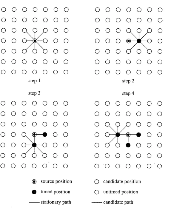
As described previously, the fundamental operation of the graph theory method is to apply a stencil at a point in the model grid for which the traveltime is b,own and then to extrapolate that time to other grid points in the immediate neighborhood. There-fore, the algorithm begins at the source location with zero traveltime and proceeds as diagramed in Figure 4. After timing points, referred to henceforth as candidates, in the neighborhood of the source, the algorithm chooses from the candidates the minimum time point and treats it as a secondary source. The stencil operation is then repeated at this point, which is removed from the candidate list, and all candidates in the neigh-borhood of the secondary source are timed again, replacing previously calculated times that exceed the newly calculated ones. At each secondary source position, the algorithm also records the "parent" source, allowing us to keep track of the first arrival ray paths. This process is repeated until all of the points in the grid have been timed.
Finite Difference Algorithm
Of the many finite difference algorithms for traveltime modeling, that of Podvin & Lecomte (1991) lays the foundation for the approach taken here. The Podvin& Lecomte algorithm can be distinguished from other finite difference approaches on the basis of a somewhat subtle characteristic. Instead of choosing a unique finite difference approxi-mation to propagate the wavefront to each point in the grid, the extrapolation method computes incremental traveltimes .using multiple, independent finite difference operators and chooses the lowest value among them. The algorithm uses up to 16 such opera-tors for 2-D grids and up to 170 operators for 3-D grids. While this scheme appears rife with inefficiency - Podvin & Lecomte implemented the algorithm on a massively parallel computer - careful application of the heap sorting algorithm greatly speeds the calculation on sequential machines. In addition, not all operators need be applied at every grid point in the model.
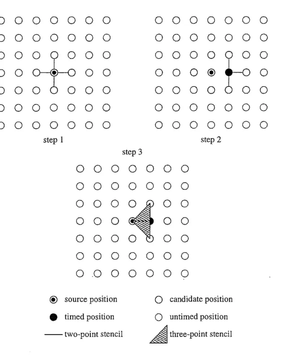
Assuming that the source position falls on a grid point, the algorithm as a first step calculates traveltimes to neighboring points along the Cartesian axes and diagonals as shown in Figure 5. Each of these points is now considered a traveltime candidate and is added to a list of candidates. The algorithm next selects the minimum traveltime point from the candidate list, removing it, and extrapolates time again using the 1-D finite different operators. In addition, 2-1-D operators are employed to extrapolate, using the original source point, the time to appropriate, neighboring gridpoints. In three-dimensional problems, 3-D finite difference operators are applied once the 2-D extrapolations have been completed. For each new and existing candidate point, the algorithm keeps track of the minimum traveltime calculated by all of the invoked op-erators. New candidate points are added to the candidate list, and the process repeats by searching the candidate list for the next minimum traveltime point.
Podvin & Lecomte incorporated additional logic in their algorithm to deal properly with head waves, owing to the fact that they represented the velocity (slowness) as a collection of constant value cells with traveltimes computed at the vertices. To avoid this added complexity, one can choose to represent the velocities at points coincident with the traveltimes. This leads to slowness averaging for the purpose of applying the finite difference operators. For finely-discretized grids, this modified algorithm yields virtually the same results as the original.
Heap Sorting
For large grids, the process of searching for the minimum traveltime among all of the can-didates can become relatively time-consuming, when compared with the computational cost of the actual extrapolation operations. To remedy this situation, Moser suggested sorting the candidate times in a "heap" (see, for reference, Knuth 1973, §5.2.3). At the expense of some computer memory, application of the heap sorting algorithm greatly enhances the speed of the traveltime modeling, making compute time nearly a linear function of the number of points in the grid.
RESULTS
Homogeneous 3-D Medium
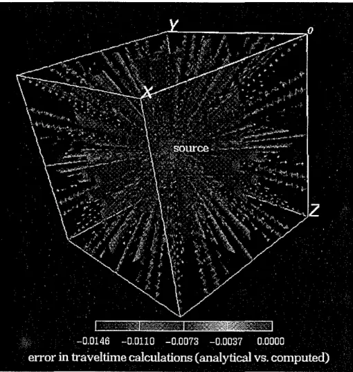
The first test of the traveltime modeling methods in three-dimensional media is to mea-sure the accuracy in a constant velocity medium. In this case the traveltime isochrons are spheres concentric about the source location. Figure 6 shows the 0.06 second isochron calculated by the finite difference method for a source at the center of cubic volume of earth with constant 4000 ftjs velocity. Each dimension of the volume is 1000 ft.
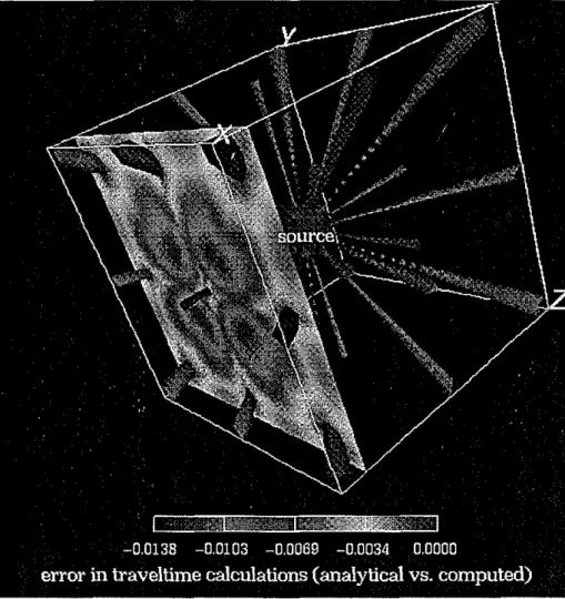
As in the two-dimensional examples presented earlier, the finite difference and graph theory methods exhibit different accuracies with regard to traveltime computations in 3-D media. Corresponding to the results illustrated in the previous figure, Figure 7 shows percent errors as a function of position in the volume. In this figure the
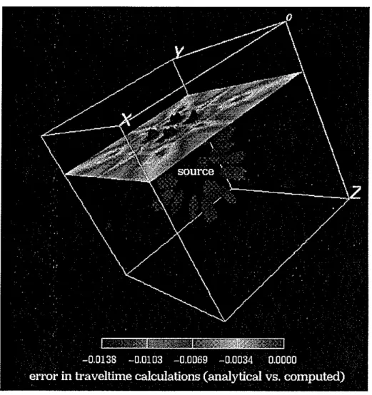
balloon-like surfaces corresponds to the largest traveltime errors. These large errors are seen to be limited in azimuth and confined to a region close to the source. This result indicates that percent error decreases with radius. The surface in Figure 8 shows directions of least error. The spikes that characterize this surface emanate from the source along the Cartesian axes and diagonals. Along these directions, the traveltimes are calculated exactly.
The graph theory method behaves differently from the finite difference method as illustrated in the percent accuracy plot of Figure 9. First, the blue surfaces that contour the largest errors and look more like cones than balloons. This is because the percent traveltime errors are not a function of radius for this calculation method. Also, the largest errors appear in sets of four cones surrounding each Cartesian axis. Typically for the graph theory method, owing to the stencils used, the directions of propagation just off-axis are modeled most poorly. In contrast, there are many more red spikes, indicating minimal error, than with the finite difference method. The graph theory stencils allow for propagation to be computed exactly in these directions.
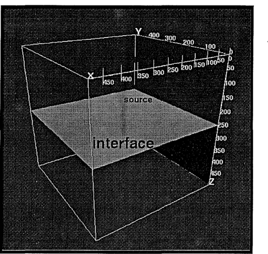
Layered 3-D Medium
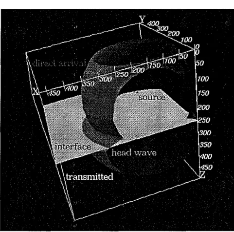
From the homogeneous medium, we move to the simple example of a highly-contrasted layered medium in order to show the traveltimes associated with more complicated wave propagation. The main purpose of this example is to demonstrate the calculation of traveltimes associated with a head wave in three dimensions. Figure 10 displays the velocity model, which comprises to layers that come together at a planar interface. The velocity above the interface is 4000 ftls, while the velocity below the interface is twice this number. Figure 10 also shows the 0.001 second (traveltime) isochron as a small sphere about the source position, which is located just above the layer boundary. In this figure the wavefront associated with the isochron has yet to impact the reflector. Figure11 presents a later isochron at 0.06 seconds in which the direct, transmitted and head wavefronts can be seen clearly. The head wave is also known as a conical wave for reasons made obvious in this figure, i.e., the head wave forms a conical "apron" about the direct arrival along the reflector. To introduce yet more complexity to the model, Figure 12 shows the same combination of direct, transmitted and head wavefronts in model where the velocity interface takes the form of a graben structure.
Computational Performance
As the preceding paragraphs focussed on issues of accuracy of traveltime calculations in three-dimensional models and the ability of the methods to model wavefield complexi-ties, e.g., head waves, the remainder of this section concentrates on the specific computer time and memory requirements for traveltime modeling. Knowledge of these require-ments allows one to extrapolate the applicability of these methods to the calculation of traveltimes for purposes of seismic imaging and tomography.
The consideration of memory requirements is straightforward. As discussed previ-ously, the amount of memory needed by both the graph theory and finite difference methods is a linear function of the number of points in the grid used to represent the slowness model. As one typically needs to store both slowness and traveltime grids in addition to accommodating the array used for heap sorting, the total memory re-quirement can be represented as
<
3 x nx x ny x nz, where nx, ny, and nz are the· number of grid points in the X, Y, and Z directions, respectively. This means that a 100 x 100 x 100 problem can be easily attempted on a computer with 12 Megabytes of memory, assuming that the calculations are performed with single precision (32-bit) floating point numbers. Given the current state of computer technology, 12 Megabytes of memory is an entirely reasonable quantity. However, if this grid were to correspond to a fixed volume of earth, and if it were deemed necessary to halve the grid discretization used in the modeling.-Le., use a 200 x 200 x 200 grid, the memory requirement would multiply by a factor of eight to 96 Megabytes, a fairly large quantity in terms of current workstation standards.The amount of time necessary to perform traveltime computations is also a linear function, or nearly so, of the number of grid points used to represent the model. This relationship is illustrated in Figure 13, which graphs the computer ("CPU") time used by the finite difference and graph theory methods on a Digital Equipment Corp. (DEC) model 3000/500 "Alpha" workstation for a variety of 3-D model sizes. The graph also includes compute time used by the finite difference method on an nCUBE Corp. model 2 processor for two model sizes-100 x 100 x 100 and 50 x 50 x 50-as well as CPU times for 2-D model computations. According to these results, the graph theory method (employing a fifth-order stencil) takes approximately seven times longer than the finite difference method to compute traveltimes for the same 3-D model. For 2-D models, this factor appears to decrease from seven to five. Also of note is the fact that for a fixed number of grid points, traveltime computations for 2-D models take much less time than those for 3-D models. This is because for both the graph theory and finite difference methods, fewer operators need to be evaluated in 2-D models at each grid point. As a final result, it appears that for the finite difference method, the calculations take six times longer on an nCUBE 2 p;ocessor (ca. 1990) than on the Alpha processor (ca: 1993). The factor of six is much smaller than floating-point performance specifications for the two processors would suggest. This is primarily because the heap sorting portion of the code is biased toward integer operations, where the disparity in processor performance is less extreme.
APPLICATIONS
The value of fast traveltime modeling is in its ability to facilitate the solution of problems in seismic imaging and tomography. In both of these applications, traveltime modeling contributes significantly to the overall solution time. Traveltimes are needed in seismic imaging in order to perform migration, a process in which the amplitudes recorded in
each seismic trace are collapsed or focused back onto the scatterer positions. In tomog-raphy, often solved by way of iterative methods such as that of conjugate gradients, traveltimes and associated paths of first arrival transmission must be repeatedly cal-culated for the iteration to converge to a stable velocity reconstruction. The following paragraphs will treat each of these applications in greater detail with specific mention of the computational requirements of realistic imaging and tomography problems.
Seismic Imaging: 2-D Pre-Stack Depth Migration
Pre-stack depth migration provides the most accurate means for imaging and character-izing subsurface reflectors from surface seismic data. A variety of approaches exist for performing this type of migration, each of which take into account differing quantities of information contained within the recorded seismic traces. A relatively robust approach involves finite differencing to backpropagate the observed wavefield into an earth model for which seismic velocities are specified a priori. A less accurate, but much faster ap-proach, is to use only traveltime information associated with the earth model to find the image points associated with strong amplitudes observed in the traces. The former approach is most appropriate when the subsurface velocities are well-understood, and a solution that is correct in amplitude remains to be found. That is to say, the solution emphasis is on the dynamic nature of the problem rather than on the kinematics. The advantage of the traveltime-only approach is in problems where the kinematics is not firmly understood, and one might wish to evaluate quickly many earth models, in order to obtain one that produces a well-resolved image of the reflectors.
Migration based on traveltimes information can be viewed as a three step process.
1. For each surface position at which a source or receiver is located, compute the traveltime from that position to all other locations in the imaging area (represented by a grid).
2. For each trace in the 'survey, sum the traveltime maps associated with the source and receiver and at each point in the imaging area place the trace amplitude associated with the two-way traveltime.
3. Stack (sum) these images to obtain the migrated section.
Amplitude corrections to better respect the propagation dynamics are often incorpo-rated into step 2. Figure 14 shows an example of the results of such a migration (bottom) for the synthetic Marmousi surface seismic dataset (bottom) with a specified velocity model (top). A 737 by 241 element grid was used to represent the velocity model and imaging area for this result, which involved the generation of traveltime information for 342 surface positions in a marine survey comprising 240 shots with 96 receivers each. The total time consumed by this process on a 256-node nCUBE 2 parallel computer (4 Megabytes memory per node) was less than 4 minutes, with a quarter of the time used in traveltime modeling and the rest used in the imaging step.
In order to extrapolate the computational requirements of a realistic 2-D problem to a realistic 3-D problem, we will consider two issues:
• The physical memory necessary to support computations on a distributed memory computer.
• The amount of computer time required to perform the traveltime modeling and imaging steps.
Representing the earth volume in terms of a 3-D grid is memory-exhaustive in that, as discussed earlier, a 100 x 100 x 100 array of single precision floating-point num-bers occupies approximately 4 Megabytes. Simultaneously storing velocity and travel-time information doubles this quantity, and the storage requirement quickly reaches the limit of physical memory available on typical workstation processors or on fine grained, distributed-memory parallel computers like the nCUBE 2. Ifthe traveltime functional varies smoothly with position, the grid discretization implied by dividing the imaging volume into a 100 x 100 x 100 array may be adequate. Ifnot, it is possible to conduct the modeling and imaging by dividing the volume into multiple slabs of equal thickness in depth. After performing the modeling and imaging for the near-surface slab, the traveltimes along the base of the slab would be used to bootstrap modeling and imag-ing in the next deepest slab. This approach assumes that the traveltime gradient with respect to depth is everywhere non-negative. This is often, but not always, the case.
Given that the earth volume can be contained within available computer memory, we have left to consider the computation time. which is a function of the grid and survey sizes. For the imaging step, this time linearly relates to the number of elements in the imaging grid, without regard to the model dimensions if simplified amplitude cor-rections are employed. In the traveltime modeling, the compute time depends linearly on the model size, but as demonstrated earlier, for a fixed number of grid elements, 3-D modeling takes longer than 2-D modeling owing to a difference in the number of extrapolators used. When confronted with the grid sizes being used currently to represent the SEG/EAEG Salt and Overthrust models for finite difference wave propa-gation simulations, it becomes readily apparent that some compromises and tricks, like those mentioned previously, need to be made in order to shoehorn traveltime model-ing algorithms onto the computer. For instance, the grid size used to represent the 13.5 x 13.5 x 4.2km deep Salt Model at 20m spacing is 676 x 676 x 211 points. Even if this entire grid (approximately 100 million points) could be fit all at once in computer memory, the compute time on a serial DEC Alpha processor would be roughly 100 times that of the 100 x 100 x 100 grid.
Tomography: 2-D Cross-Well Traveltime Inversion
Seismic tomography, as a form of inversion, is a step beyond seismic imaging when it comes to algorithmic complexity. Whereas the migration discussed previously involves an instance of traveltime modeling to simulate the propagation of seismic waves through
a subsurface of known velocity and an instance of imaging to collapse the trace ampli-tudes to reflector positions, tomography requires repeated instances (an iteration) of these two steps. The iteration can constitute a gradient algorithm yield the final to-mogram through a sequence of perturbations starting with an initial velocity model, or the iteration can take the form of a· Monte Carlo approach, where models are pseudo-randomly chosen and tested for goodness of data fit. Either way, this often entails tens, hundreds and possibly thousands or more modeling and backprojection steps.
The gradient algorithm for solving the nonlinear tomography inversion takes the form of a single iteration loop as shown in Figure 15. Ray tracing and traveltime computation provide the first step. Residual calculation and backprojection act as the second and third steps, respectively. And the algorithm incorporates a condition for deciding when the reconstruction is complete. If incomplete, the model is updated and the iteration continues. With each model change, rays are retraced rays and new traveltimes obtained. Often, this re-computation of traveltime and raypaths can be restricted to iterations that follow significant model changes.
MIT's Michigan Basin cross-well survey provides an example application of seismic traveltime tomography to real field data. In the Michigan survey, the dataset comprised 20,547traveltime picks culled from 201 sources and 201 receiver positions. The velocity model used to describe the carbonate reef complex buried among horizontally layered sediments was represented on a 141 (width) x 154 (height) grid. Starting from a layered background model, the conjugate gradient solver used to obtain the final tomogram required 150 iterations, not all of which involved ray tracing/traveltime modeling. This number of iterations translated to a compute time of several hours to obtain complete convergence. Each instance of traveltime/ray modeling (applying the graph theory approach) required less than a minute, assuming one source position per processor on the nCUBE 2. In contrast, each instance of slowness integration over fixed rays required a fraction of a second. Figure 16 shows the a diagram of the survey geometry, along with the final tomogram and geologic interpretation.
For reasons of survey cost and questionable resolving power, 3-D well-to-well tOe mography may not ever become a commercially popular technique, but 3-D refraction tomography has already evoked interest in the petroleum industry for dealing with the surface statics problem. The basic process is to take the surface seismic data, pick traveltimes associated with turning rays and possibly shallow reflections, and use this information to obtain near surface velocity. As in the case of seismic imaging, the com-putational tractability of this type of tomography depends on memory requirements and processor time. The memory requirement issue for tomography is similar to that of seismic imaging except that more information must be stored at each point in the grid. In addition to the slowness and traveltime, one typically records raypath information and several buffers of model gradient information needed in the conjugate gradients method. In terms of computer time, it is reasonable to expect that, at worst, typical tomography inversions (not including associated uncertainty analyses) will run N times longer than typical seismic migrations, where N is the number of iterations to reach
convergence.
CONCLUSIONS
The finite difference and graph theory methods allow traveltime modeling to be per-formed extremely quickly, facilitating such applications as seismic imaging and tomog-raphy. Both methods are typically used to compute first arrivals, but through the incorporation of reflector information into the earth model, later arrivals can also be simulated. For the same amount of computational expense, the finite difference algo-rithm tends to achieve significantly greater traveltime accuracy. This makes the finite difference method the preferred approach for seismic imaging applications, where only traveltime information is needed. The ability of the graph theory method to efficiently compute and record raypath information perhaps makes it the preferred approach for seismic tomography applications in which raypaths are needed.
To allow for complicated propagation in highly heterogeneous media, both finite difference and graph theory algorithms can be made to incorporate heap sorting so that traveltime extrapolation can be efficiently carried out along the wavefront. Even with heap sorting, the algorithms have the nice property that the computational time and memory requirements scale linearly with the number of grid points used repre-sent subsurface velocities in discrete form. Realistically-sized two-dimensional seismic surveys can be simulated in reasonable time on current supercomputers. For realistic three-dimensional seismic surveys, the computational memory and time requirements somewhat exceed the capacity of the largest existing supercomputers and workstation networks. However, it is straightforward to predict the computer resources that will be required to address these problems, and it is likely that these computer resources will become available in the near future. In addition, current efforts to simulate large seismic surveys will eventually provide the datasets to test predictions.
REFERENCES
Aki, K. and P. Richards, Quantitative Seismology, Theory and Methods, va!. 2, W. H. Freeman and Co., New York, 1980.
Asakawa, E. and T. Kawanaka, Seismic raytracing using linear traveltime interpolation, inEuropean Assoc. Exploration Geophys. 1991 Meeting, EAEG, Zeist, Netherlands, 1991, Abstracts.
Dijkstra, E., A note on two problems in connection with graphs, Numer. Math., 1, 269-271, 1959.
Itoh, K. ,H. Saito, and H. Yamada, A method for approximate computation of first ar-rival traveltimes in seismic refraction modeling, in Soc. Exploration Geophys. Japan, Proc. 1983 Spring Meeting, pp. 11-12, SEGJ, 1983.
Knuth, D. E., Sorting and Searching: The Art of Computer Programming, va!. 3, Addison-Wesley, 1973.
MandaI, B., Forward modeling for tomography: triangular grid-based Huygens' princi-ple method, J. Seis. Expl., 1, 239-250, 1992.
Moser, T., Shortest path calculation of seismic rays, Geophysics, 56, 59-67, January 1991.
Podvin, P. and 1. Lecomte, Finite difference computation of traveltimes in very
con-trasted velocity models: a massively parallel approach and its associated tools, Geophys. J. Int., 105, 271-284, 1991.
Qin, F., K. Olsen, Y. Luo, and G. Schuster, Solution of the eikonal equation by a finite difference method, in Proc. Soc. Exploration Geophys., 1990 Meeting, pp. 1004-1007, Tulsa, OK, 1990, SEG, Expanded abstracts.
Saito, H., Traveltimes and raypaths of first arrival seismic waves: computation method based upon Huygens' principle, in Soc. Exploration Geophys. 1989 Meeting, pp. 244-247, SEG, Tulsa, OK, 1989, Expanded abstracts.
van Trier, J. and W. Symes, Upwind finite-difference calculation of traveltimes, inProc. Soc. Exploration Geophys., 1990 Meeting, pp. 1000-1002, Tulsa, OK, 1990, SEG, Expanded abstracts.
Vidale, J., Finite-difference calculation of travel times, Bull. Seis. Soc. Am., 78, 2062-2076, 1988.
Graph Templates
Sthorder 4thorder 3rdorder 151order 2nd order~
L
k:
lie = 90" lie = 45" 88 . = 18.4"mm 88 . =7.1"moo 88 . = 3.2"moo
88 = 26.6" lie = 18.40 lie =14.0°
mox mox mox
6thorder (pruned)
I Othorder (pruned)
88 .moo=4.3"
88mox=6.3"
Homogeneous Model
Graph (order=5) offset (m)o
250 500 750 1000 0.9 0.8 0.7 0.6~
~ 0 0.5 t:""
Ei 0.4 .", 0; 1; 0.3'"
0.2 0.1 0Figure 2: Traveltime error associated with a fifth-order stencil operator used in the graph theory method. In effect, exact traveltimes are calculated for points within a radius of20m of the source.
Figure 3: Traveltime error associated with finite difference extrapolation. Exact travel-times were explicitly calculated for points within a radius of20m of the source.
Extrapolation Process
0
0
0
0
0
0
0
0
0
0
0
0
0
0
0
0
0
0
0
0
0
0
0
0
0
0
0
0
0
0
*
0
0
0
0
0
*
0
0
0
0
0
0
0
0
0
0
0
0
0
0
0
0
0
0
0
0
0
0
0
0
0
0
0
0
0
0
0
0
0
0
0
0
0
0
0
0
0
0
0
0
0
step 1 step 2 step 3 step 40
0
0
0
0
0
0
0
0
0
0
0
0
0
0
0
0
0
0
0
0
0
0
0
0
0
0
0
0
0
0
0
0
0
0
0
0
0
0
0
0
~
0
0
0
0
0
0
0
0
0
0
0
0
0
0
0
0
0
0
0
0
0
0
0
0
0
0
0
0
0
0
0
0
0
0
0
0
0
0
@ source position
0
candidate position•
timed position0
untimed position - - stationary path - - candidate pathExtrapolation Process
0
0
0
0
0
0
0
0
0
0
0
0
0
0
0
0
0
0
0
0
0
0
0
0
0
0
0
0
0
0
~
0
0
0
0
0
0
H
0
0
0
0
0
0
0
0
@0
0
0
o
0
0
0
0
0
0
0
0
0
0
0
0
0
0
0
0
0
0
0
0
0
0
0
0
0
0
0
0
0
0
0
0
0
0
0
0
step I step 2 step 30
0
0
0
0
0
0
0
0
0
0
0
0
0
0
0
0
~
0
0
0
0
0
0
0
0
0
0
0
0
0
0
0
0
0
0
0
0
0
0
0
0
0
0
@ source position
o
candidate position•
timed positiono
untimed position- - two-point stencil
~
three-point stencilFigure 6: 'Traveltime isosurface in homogeneous medium.
Figure 7: Percent error isosurface (spines) for finite difference method showing directions of greatest accuracy. Plane orthogonal to X-axis shows percent error as function of position.
Figure 8: Percent error isosurface (balloons) for finite difference method showing regions of least accuracy. Plane orthogonal to Z-axis shows percent error as function of position.
Figure 10: 3-D layered model with planar boundary between low velocity (4000 ftls medium on top and high velocity (8000 ft/s) medium at the bottom. Isochron shows wavefront (aspherical owing to coarse sampling of isosurfacing algorithm) in vicinity of
Figure 11: 0.06s isochron showing wavefront in far field of source. Traveltime isosurface comprises direct, transmitted, and head wave.
50
Figure 12: 0.06 s isochron showing a somewhat complicated wavefront emanating from a source location above a graben structure with highly contrasted velocity.
3-D Modeling Perfonnance
1500•
• ••
,P
S -...
Finite Difference 0 / on-
Graph Theory / 0 D -o 0 / fl M ro - 0 - FD (nCUBE) / /-&
1000-
/ /.
:;;:
/ / U / I.Il / / Q P /"
0 / / /"
"
500 f- / /.
~ / /"
.§
c f / / / GT (2-D) ::> "/ _..Q (206 s.)'"
!if
-U
--.-..
FD (2-D) • A- ~ . . - • •a
(44.7 s.) 010° 2105 4105 6105 8105 1 106 #of pointso 8
'"
8 o'"
o::::
0 8 0 0 ~O ~O...
...
5'"
5'"
cd"
"
l-< ..el ..el Of) ~ ~ 0 0'S
...
[/). ;i 0~
0 0:;s
0 0'"
'"
'"
'"
depth (m) depth (m)Figure 14: An example of the results of 2-D Kirchhoff pre-stack depth migration (bot-tom) for the synthetic Marmousi surface seismic dataset with a specified velocity
struc-<itart: k=O
~
raytrace /" (G k,dkI mk) k=k+1 compute residual ( 8dkI dk ' dabs) backproject ( 8mk I 8dk ' Gk ) step calculation ( ak 1Gk ' 8mk ) 18mkI update model (and I 8dk I) .no (mk+118mk ' mk ) small? yesFigure 15: Shown in flowchart form, the gradient algorithm for solving the nonlinear tomography inversion takes the form of a single iteration loop.
Raypath Coverage Michigan Inversion [Constant17kftlsstarting] offset(tt) offset(ft)
"
SOO 1000 1500 0 500 1000 1500 3500 3500 22000 4000 4000 20000~ ~ ~"
.g " S ~ ~ § 4500 4500 5-'"
2 18000] 0 > 5000 5000 16000 5500 ssoo 14000"
500Michigan Test Site Geology
Burnt Bluff Cnrbonnle Vp=21,500 fils
Brown Niaga;.an (Reservoir)" 2000 MITlStech J·2IA (source well) Vp =21,3 I Vp=21,SOOW Vp=19,000Ws V =2 OOOftls offset(ft) UIOO 1500 :Shell well : Vp= 14,4lJO!lJs
•
500 trin eri '" FSall I.
,
EUnit Shale rmgerIn BSait Gray Niagaran Schoolcraft Carbonate MlTlBurch 1·20B (receiver well) ~ 0 ~ ~...
I;; ~ ~ § ~ 8 0 ll: 8Figure 16: The Michigan Basin field survey geometry (top left), along with the final tomogram (top right) and geologic interpretation (bottom).