HAL Id: hal-01190664
https://hal.archives-ouvertes.fr/hal-01190664
Submitted on 1 Sep 2015
HAL is a multi-disciplinary open access
archive for the deposit and dissemination of
sci-entific research documents, whether they are
pub-lished or not. The documents may come from
teaching and research institutions in France or
abroad, or from public or private research centers.
L’archive ouverte pluridisciplinaire HAL, est
destinée au dépôt et à la diffusion de documents
scientifiques de niveau recherche, publiés ou non,
émanant des établissements d’enseignement et de
recherche français ou étrangers, des laboratoires
publics ou privés.
Selection of appropriate calculators for landscape-scale
greenhouse gas assessment for agriculture and forestry
Vincent Colomb, Ophelie Touchemoulin, Louis Bockel, Jean Luc Chotte,
Sarah Martin, Marianne Tinlot, Martial Bernoux
To cite this version:
Vincent Colomb, Ophelie Touchemoulin, Louis Bockel, Jean Luc Chotte, Sarah Martin, et al..
Selection of appropriate calculators for landscape-scale greenhouse gas assessment for
agricul-ture and forestry. Environmental Research Letters, IOP Publishing, 2013, 8 (1),
�10.1088/1748-9326/8/1/015029�. �hal-01190664�
This content has been downloaded from IOPscience. Please scroll down to see the full text.
Download details:
IP Address: 147.99.35.145
This content was downloaded on 07/01/2014 at 07:49
Please note that terms and conditions apply.
Selection of appropriate calculators for landscape-scale greenhouse gas assessment for
agriculture and forestry
View the table of contents for this issue, or go to the journal homepage for more 2013 Environ. Res. Lett. 8 015029
(http://iopscience.iop.org/1748-9326/8/1/015029)
IOP PUBLISHING ENVIRONMENTALRESEARCHLETTERS
Environ. Res. Lett. 8 (2013) 015029 (10pp) doi:10.1088/1748-9326/8/1/015029
Selection of appropriate calculators for
landscape-scale greenhouse gas
assessment for agriculture and forestry
Vincent Colomb
1, Oph´elie Touchemoulin
2, Louis Bockel
2,3,
Jean-Luc Chotte
1, Sarah Martin
4, Marianne Tinlot
2and
Martial Bernoux
11IRD, UMR Eco&Sols (Montpellier SupAgro, CIRAD, INRA, IRD), 2 Place Viala, F-34060
Montpellier Cedex 2, France
2FAO, Policy and Programme Development Support Division, Policy Assistance Support Service
(TCSP), via delle terme di Caracalla, I-00153 Rome, Italy
3FAO, Agricultural Development Economics Division (ESA), Economics of Sustainable Agricultural
Systems (ESAS), via delle terme di Caracalla, I-00153 Rome, Italy
4ADEME, Service Agriculture et Forˆets, 20 avenue du Gr´esill´e - BP F-90406 - 49004 Angers cedex 1,
France
E-mail:martial.bernoux@ird.fr
Received 13 January 2013
Accepted for publication 18 February 2013 Published 7 March 2013
Online atstacks.iop.org/ERL/8/015029 Abstract
This letter is intended to help potential users select the most appropriate calculator for a landscape-scale greenhouse gas (GHG) assessment of activities for agriculture and forestry. Eighteen calculators were assessed. These calculators were designed for different aims and to be used in different geographical areas and they use slightly different accounting methodologies. The classification proposed is based on the main aim of the assessment: raising awareness, reporting, project evaluation or product assessment. When the aims have been clearly formulated, the most suitable calculator can be selected from the comparison tables, taking account of the geographical area and the scope of the calculation as well as the time and skills required for the calculation. The main issues for interpreting GHG assessments are discussed, highlighting the difficulty of comparing the results obtained from different calculators, mainly owing to differences in scope, calculation methods and reporting units. A major problem is the poor accounting for land use change; the calculators are usually able to account satisfactorily for other emission sources. One of the main challenges at landscape-scale level is to produce a realistic assessment of the various production systems as the uncertainty levels are very high. The results should always give some indication of the link between GHG emissions and the productivity of the area, although no single indicator is able to encompass all the services produced by agriculture and forestry (e.g. food, goods, landscape value and revenue).
Keywords: landscape, carbon calculators, greenhouse gases, GHG emissions, AFOLU, mitigation S Online supplementary data available fromstacks.iop.org/ERL/8/015029/mmedia
Content from this work may be used under the terms of theCreative Commons Attribution 3.0 licence. Any further distribution of this work must maintain attribution to the author(s) and the title of the work, journal citation and DOI.
1. Introduction
Climate change and its consequences are recognized as one of the major environmental challenges for this century. The Intergovernmental Panel on Climate Change (IPCC) identified
1
agriculture, forestry and other land use (AFOLU) as one of the main sources of GHG emissions.
AFOLU represents about 30% of the total GHG emissions worldwide. The contribution of agriculture to GHG missions from each country depends mainly on the structure of the economy. Excluding land use change and forestry (LUCF) this varies from a few per cent (e.g. 1% for Jordan in 2000, 6% for the USA in 2010) to half, or more, of total emissions (e.g. 48% for Brazil in 2005, 68% for Benin in 2000, 91% for Chad in 1993) (UNFCCC2012).
Land use change (LUC) also plays a major role in GHG emissions, causing significant changes in carbon pools, leading to large-scale emission or storage of CO2. Globally,
deforestation alone accounts for 11% of anthropogenic GHG emissions (Van der Werf et al 2009). LUC is critical for environmental assessment as shown by the opposition to biofuel production which is increasing pressure on forests in South America and Asia (Lambin et al 2001, Lapola et al 2010, Plevin et al 2010). LUC includes direct LUC (dLUC), occurring in the study area itself, and indirect LUC (iLUC), occurring outside the study area but resulting from changes within the study area. Including iLUC in environmental assessment involves many assumptions about the socio-economic relationships between different areas. Depending on the assumptions made, some studies have shown that indirect emissions can be greater than local GHG savings (Fargione et al 2008). However, the assumptions underlying indirect emissions need to be studied and improved (Kim and Dale2011). Several methodologies for quantifying the impact of dLUC and iLUC are currently being proposed and discussed as part of the development of consequential assessment approaches (Thomassen et al2008, Brander et al 2009). ‘Consequential assessment’ focuses on the impacts of changes and the relationships between production systems and is a useful approach for evaluating the effects of policies. ‘Attributional assessment’, on the other hand, is useful for comparing the emissions from the processes used to produce (and use and dispose of) different products (Brander et al 2009).
This study focuses on GHG assessment at landscape scale (Milne et al2012). Here, landscape scale starts above the scale of a single farm and can reach national scale. Landscape scale is being adopted to an increasing extent for GHG assessment and GHG policy planning (Milne et al2012) and can be more cost effective and less time consuming than GHG assessments for individual farms. Moreover, working at landscape scale can reinforce networks, upgrade skills within the groups involved and encourage mitigation initiatives (Milne et al 2012). Implementing mitigation strategies at landscape scale increases the potential for mitigation compared to individual farm strategies. It facilitates access to carbon markets and subsidies or other incentives, and spreads the costs. Working at landscape scale is also relevant as AFOLU activities are often interdependent within an area (Milne et al2012).
There is an increasing demand by project managers and policy makers for suitable GHG assessment tools to reap the benefits of a landscape-scale approach. Assessments are often carried out by agronomists, land managers, NGOs
and technical institutes who are not specialists in GHG accounting. The IPCC has published guidelines and good practices for GHG accounting (IPCC 2006) and various tools have been developed to help those performing GHG assessment within these guidelines. These tools provide a framework for the assessments and a database of emission factors Denef et al (2012) classified these tools into calculators, protocols, guidelines and models. This review focuses on calculators (automated web, Excel or other software-based calculation tools) that have been developed for quantifying GHG emissions and removals by AFOLU.
This letter provides guidance for potential users in selecting the most appropriate calculator for their aims and requirements. The discussion covers the major methodological differences between these calculators and considers comparability issues. This letter also sets out to improve transparency in GHG and carbon analysis, improve the analysis of results by end users and provide ideas for further development of GHG and carbon calculators.
2. Materials and methods
A literature search was carried out in English, French and Spanish and a large number of GHG calculators for AFOLU were identified. Many calculators have been developed for internal use by private companies or consultancies: these have not been included. Many of the calculators identified were product specific (milk, meat, cereals, wood etc). Only a few covered a range of activities (arable, forestry, deforestation, livestock etc) and were suitable for landscape-scale assessment.
This study focuses on landscape-scale GHG assessments accounting for all AFOLU emissions from a defined area. However, where calculators designed specifically for landscape-scale approaches are not available, large areas may be considered as a farm covering a whole region or even a country. This study, therefore also includes some farm-scale calculators, provided that they consider arable farming, livestock farming and forestry.
Only 18 multi-activity calculators were selected from the original list, namely ALU (Ogle 2011); AFD Calculator (AFD 2011); CALM (The Country Land and Business Association—CLA 2012), Carbon Calculator for New Zealand Agriculture and Horticulture (Lincoln University 2008), Carbon Farming Group calculator (Carbon Farming Group 2012), Carbon Benefit Project calculator for simple assessment (Carbon Benefits Project2012), Climate Friendly Food carbon calculator (CFF 2010), ClimAgri R
(ADEME 2011a), Cool Farm Tool (Hillier et al2011), Cplan v2 (Dick et al 2008, CPLAN 2012), Dia’terre R (ADEME 2011b), EX-ACT (Bernoux et al2010, FAO2012), FarmGAS (Aus-tralian Farm Institute 2009), Farming Enterprise Calculator (Queensland University Australia2011), FullCAM (Richards 2001), Holos (Little et al2008), Illinois Farm Sustainability (IFS) Calculator (McAvoy et al2009), USAID FCC (USAID 2013). Most of these calculators are available free and can be downloaded directly from the websites or by contacting the developer (see supplementary material table S1 available
Environ. Res. Lett. 8 (2013) 015029 V Colomb et al
atstacks.iop.org/ERL/8/015029/mmedia). Most of them have not been published in peer reviewed journals but a description can be found on the web or in reports. All the calculators selected were tested on basic study cases to determine their features, the main inputs required and outputs provided. The methodological and practical aspects of the calculators were compared. The methodological aspects such as geographical areas for which they were suitable, scope, reporting units and features were assessed using the documentation provided with each calculator. User friendliness is more subjective and is, therefore, our personal evaluation. The assessment of each calculator was checked and updated using questionnaires filled in by the developers. The interpretation and summary is based on personal assessments by the authors, resulting from their own experience and discussions with experts in GHG assessment for AFOLU.
3. Results
3.1. Generic and specific methodologies used by the calculators
All the calculators identified are based on the IPCC guidelines and follow the IPCC tier classification. Tier 1 corresponds to very large-scale approaches, with average emission factors for large eco-regions of the world. Tier 2 is similar but uses data specific to a state or region, with more accurate emission factors. Tier 3 is a very detailed approach, usually including biophysical modelling. At the moment, Tier 3 process-based models are only available for a small number of emission sources (e.g. enteric fermentation or N2O soil emissions from
nitrification or denitrification) and limited to either a specific region (in most cases temperate regions) or a specific product (e.g. dairy cattle or flooded and irrigated rice).
For most GHG emissions (CO2 from combustion, N2O
and CH4), the IPCC generic approaches (Tiers 1 and 2)
are based on multiplying an emission factor for a given gas and source category by activity data for the emission source (e.g. the area, the number of animals, the mass or volume of fuel). For CO2emissions related to LUC (a change
from one IPCC category to another—forest land, cropland, grassland, wetlands, settlements, other land—IPCC 2006) or due to change of management within one category (e.g. tillage to no-tillage for cropland), IPCC recommends a mass balance approach based on carbon stock changes over time for 5 compartments: above-ground biomass, below-ground biomass, litter, dead wood and soil.
Global calculators tend to use the Tier 1 approach, whereas regional calculators tend to combine Tiers 1 and 2. Some regional calculators use Tier 3 with a modelling approach (e.g. Cool Farm Tool, US cropland calculator). The calculators require pedo-climatic and management inputs. Each calculator has a slightly different input dataset depending on its features, the default data provided and the tier selected. All the calculators use a year as the unit of time and a hectare as the unit of area.
3.2. Geographical coverage of the calculators
All the calculators identified were developed by teams from Annex 1 countries, as defined in the United Nation Framework Convention on Climate Change (industrialized countries), and most focus on industrial agriculture. Most calculators were also designed to be used for a particular country (e.g. Climagri R
was developed for France), although some can be used anywhere in the world (e.g. Ex-act), and others were designed only for regional use (e.g. Farming Enterprise Calculator). Calculators developed for ‘low income countries’ focus on development projects and clean development mechanisms (CDM). Some emerging countries with strong export activities, such as Chile and South Africa, are developing their own calculators for their main products. Some regional calculators may have been missed by the search if they were not developed in English, French or Spanish.
When possible, calculators designed for landscape scale should be given priority for landscape-scale GHG assessment, but some farm-scale calculators may be a useful alternative.
3.3. Scope of the calculators
The scope corresponds to the limits of the processes included in each calculator as it is defined for life cycle assessment (LCA) in ISO 14040:2006. The scope can be divided into two levels: the activities and the sources accounted for within each activity. Activities here refer to the main production system. Almost all calculators account for temperate crops, grassland, dairy cattle and other livestock. About half account for perennial farming and forestry, whereas very few account for tropical crops, rice, horticulture and trees and hedges (see supplementary material table S2 available at stacks.iop.org/ ERL/8/015029/mmedia).
For each activity, the major sources (soil N2O from
fertilizers, enteric CH4 and manure CH4) are accounted
for by almost all of the calculators. Additional sources are, in general, considered, but not uniformly. CO2 from
energy consumption (fuel and electricity), N2O from residues,
off-farm emission (fabrication of inputs and feed), CO2
sink/source from changes in the soil or the biomass and CH4
from peat are included in many calculators. CO2 associated
with machinery and infrastructure, N2O from leguminous N
input, CH4and N2O from biomass burning, CH4from flooded
rice, CO2from off-farm processing, CO2from transport and
GHG savings from renewable energy production are rarely included (see supplementary material table S3 for details available atstacks.iop.org/ERL/8/015029/mmedia).
3.4. Aims of GHG assessments
GHG assessments can be undertaken for various reasons. The following simplified classification is proposed (cf supplementary material table S4 available at stacks.iop.org/ ERL/8/015029/mmediafor overview):
• Raising awareness.
This covers assessments whose main purpose is education about climate change and the role of agriculture. They are mainly carried out by farmers and farming consultants. They require very simple calculators for which little or no training is required. They are user friendly and can identify major sources of emissions. They are often in the form of free, online calculators. Typically, they use a Tier 1 approach and have a large uncertainty. Most of them exclude soil carbon stocks and LUC. The Carbon Calculator for New Zealand Agriculture and Horticulture, the Farming Enterprise GHG Calculator, the simplified version of Cplan (Cplan v0) and specialized arable farming calculators such as US cropland GHG calculator (McSwiney et al2010) are typical examples.
• Reporting.
This covers accurate, exhaustive assessments of the status of a study area, to enable comparisons to be made between countries or farms. Such assessments are usually carried out by trained technicians or consultants. The results are used by policy makers to design appropriate programmes. The calculators may be designed for landscape scale or farm scale and must take account of the diversity of management practices in the study area. They may use Tier 1 or Tier 2 approaches. Subcategories can be defined depending on the scale.
∗ Landscape-scale calculators. These are designed to meet official requirements for GHG assessment. These calculators must avoid double accounting and conform to official standards. The results have a high uncertainty due to the uncertainty of both the activity data and the emission factors. These calculators use averaged data and can be quite time consuming, especially for data collection. ALU, Climagri R and FullCam are in this subcategory.
∗ Farm-scale calculators. These are designed to help farmers identify the main emission sources on their farm, which is the first step before implementing a reduction strategy. However, these calculators are not really designed to assess changes. Diaterre R
, CALM, CFF Carbon Calculator and IFSC are in this subcategory.
• Project evaluation.
This covers assessments of the impact of a project or a policy in terms of GHG emissions. These assessments can be carried out by policy makers, NGOs, technicians or consultants. Calculators for project evaluation compare a baseline (a business-as-usual scenario) to an ‘end of project’ situation. The design of the calculator depends on the type of project to be assessed: climate change mitigation or agricultural development. These calculators should account for all possible mitigation options, including carbon storage. They can be split in two subcategories, depending on whether they are carbon market oriented. Carbon market oriented assessments require a higher level of skill.
∗ Carbon market projects. These calculators have been designed mainly for countries where agriculture is involved in a carbon market or where there are potential CDM projects. For farming, FarmGAS and the Carbon Farming Group calculator are in this subcategory, as are dedicated specific afforestation/reforestation calculators such as TARAM and ‘CO2fix’.
∗ Other projects. These calculators usually account for all possible mitigation options, especially carbon storage. However, they need to be cost effective and user friendly. They aim to provide information for project managers, decision makers and aid agencies. EX-ACT, USAID FCC, CBP and Holos are in this subcategory. • Product assessment.
This covers assessments used mainly by private businesses to analyse impacts along a value chain and improve a product’s carbon footprint. The principal aim of the calculators is to compare different products rather than assessing the emissions from an area and they are, therefore, designed to provide a GHG assessment for a single product. They reveal the relationship between production levels and emissions. Usually these calculators include processing and transport. Only 2 of the 18 calculators evaluated are in this category: Cool Farm Tool and Diaterre R. Most current LCA calculators with their associated databases (e.g. SimaPro—Rice et al1997) are in this category.
3.5. Time and skills required
There are significant differences in the time and skills required for the various calculators. Some are very easy to use and very little time is needed to collect the data required whereas others require much more time and skills table1. It is difficult to give a precise estimate of the time necessary for each calculator, as it is very dependent on the level of accuracy and reliability and the availability of the data for each assessment. Both agronomy/forestry skills and computer skills are required to use the calculators.
4. Discussion
4.1. Scope
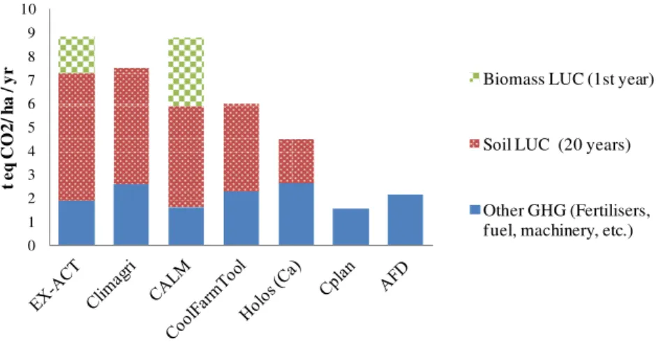
Differences between the scope for each calculator prevent di-rect comparison of the assessments using different calculators. The exclusion of LUC emissions can have a significant impact on the results, especially for deforestation/reforestation or changing grassland to annual crops or settlements As an example, seven calculators were used to assess the GHG balance of a simple system: the replacement of established grassland by wheat (in European conditions) (figure 1). Figure 1 shows that the LUC emissions are higher than the emissions from the wheat production itself (fuel, fertilizers and pesticides). Very few calculators fully account for the emissions from the loss of previous biomass. CO2 soil
Environ. Res. Lett. 8 (2013) 015029 V Colomb et al
Figure 1. Mean annual net GHG emissions for wheat sown on grassland in temperate conditions (mainly Europe). Table 1. Time and skills required. (Legend: + to ++++; from slowest (>1 month) and most difficult (formal training required) to the fastest (<1 day) and easiest to use.)
Calculator Speed of assessment Ease of use
AFD calculator +++ ++++
ALU + +
CALM +++ +++
Carbon benefit project CPB ++ ++
Carbon Calculator for NZ Agriculture and Horticulture ++++ ++++ Carbon Farming Group Calculator ++++ ++++
CFF Carbon Calculator +++ ++
Climagri R + +
Cool Farm Tool +++ +++
CPLAN v2 +++ +++
Dia’terre R +++ +
EX-ACT ++++ +++
FarmGAS ++ ++
Farming Enterprise Calculator ++++ ++++
FullCAM + +
Holos ++ +++
IFSC ++++ ++
USAID FCC ++++ +++
tested. However, the values differed significantly between the calculators. CO2soil emissions are considered to occur over
a period of 20 years on average (IPCC 2006). Cplan and USAID FCC ignore emissions from LUC. This example also shows the importance of considering the period over which the emissions occur, as calculators that do not take account of time are unable to estimate LUC emissions.
Most calculators are designed to exclude LUC for practical reasons, methodological complexity or because the effect is not permanent (LUC is reversible). Direct LUC (dLUC), can be observed and accounted for objectively for projects and policies that include LUC incentives. However, changes in the study area will also affect other areas, especially if the demand for food products is non-elastic. Assuming a constant or increasing food demand implies that, if food production decreases in one area, other areas will have to compensate for the loss by intensifying the farming systems or by increasing the cropping area (indirect LUC, iLUC). If the existence of a compensation mechanism is assumed then indirect emissions must be taken into account if there is a reduction in production levels. Assessments
including iLUC must use economic modelling or be based on expert knowledge (Fargione et al2008, Kim and Dale2011). Global food balance is not the only driver for LUC which is influenced by many factors. Initial land profitability (usually zero for forests), land tenure, production and investment capacities and state regulations may be as important as the price of food products. Furthermore, food demand is slightly flexible, as many food products can be replaced by products that use fewer natural resources (e.g. replacing protein from meat with vegetable protein) and so it is difficult to establish a clear consequential relationship between changes in one area and changes in others, sometimes thousands of km away (e.g. biofuels, soya beans for European cattle). It is, therefore, not surprising that, at the moment, only dLUC is accounted for in the calculators. It is likely that indirect LUC will be included in the near future, providing useful information in conjunction with the consequential assessment methods being developed (Brander et al2009). However, indirect LUC emissions would need to be reported separately as they have a very high uncertainty.
Table 2. Main sources of GHG for AFOLU activities. Production Major sources that may need to be accounted for
Arable crops N input from fertilizer, N input from crop residue decomposition, Methane emissions from irrigated or flooded rice production, land use change (particularly peat land conversion) and management change (tillage, impact on soil carbon stock).
Livestock Enteric fermentation, Management of manure (both dung and urine) and accounting for use of organic manure. Feeding practices and accounting method for imported food (share of pastures).
Horticulture Organic soil, energy and infrastructure.
Forest Biomass and soil carbon, plantation versus natural forest, land use change.
Another source of difference between calculators is the handling of N2O emissions which can differ significantly
depending on the individual sources of N considered. The main difference is between calculators accounting for only mineral and/or organic N fertilizers and others accounting for N from crop residues and nitrogen deposition in addition. The N sources accounted for should be checked when using calculators and analysing the results. The IPCC recommends that all sources of N should be included except N from leguminous fixation. Some calculators differentiate between direct and indirect N2O emissions, thus accounting for
volatilization and re-deposition processes. This step is not considered to modify the overall N2O balance. One main
difference in results might come from crop residue emissions. For instance, in a case study in the Brittany region of France, crop residues were estimated as representing 14% of all N inputs (Sarah Martin, personal communication). Many calculators have incomplete coverage of N sources and need to be extended and so users must be careful in their interpretation of N2O emissions (see supplementary material
table S3 available atstacks.iop.org/ERL/8/015029/mmedia). On-farm processing is often partially considered but poorly identified in carbon calculators. It might have a significant potential for mitigation but is probably better considered at farm scale rather than at landscape scale. One important option for decreasing agricultural carbon footprints is to reduce post-harvest losses. No calculator yet includes post-harvest losses although these could be taken into account by considering yields of the value chain right up to the end-user rather than yields at the field or to the farm gate.
Finally, every GHG calculator accounts for slightly different sources. The major sources of emissions which deserve special consideration in GHG assessments depend on the production systems. Potential users of the calculators need to check that the key sources (see table2) are accounted for by the calculators when there is significant production in the area studied.
4.2. Units for GHG accounting
The various units used by calculators to report the results might be a source of confusion. Results are expressed in tons of CO2 equivalent per year, per project, per unit area or per
unit of production (table S5 available atstacks.iop.org/ERL/ 8/015029/mmedia). The results may be expressed as a net value (emissions–removals) or as both values. Users must also be careful not to confuse tons of carbon and tons of
CO2 equivalent (conversion factor 44/12). Some calculators
provide results only for a given situation, while others provide values for an initial situation, the baseline, and an ‘end of project’ situation.
The simplest reporting unit for landscape-scale GHG assessment is the quantity of GHG expressed in CO2
equivalent per ha. However, this unit is not suitable for livestock production systems and is not associated with the production level of the area.
When considering the most suitable unit for the results, a distinction should be drawn between ‘low’ and ‘high’ productivity areas. Given the global context with increasing demand and the possibility of leakage (indirect emissions), different indicators are required for ‘medium and large-scale industrial agriculture’ and for ‘small-scale’ agriculture.
Medium and large-scale agriculture is clearly market oriented, has a high level of production and provides a considerable proportion of the total food required for human consumption. The main environmental challenge here is to reduce the carbon footprint per ‘unit of production’. Calculators use several units to associate the emissions with the production level: LCA calculators tend to express the results in GHG per kg of product, Climagri R produces a ‘Territory Feeding potential indicator’, Audsley and Wikinson (2012) suggest expressing the GHG emissions with respect to metabolizable energy and crude protein. It is difficult to assess agricultural systems with many different outputs at landscape scale. For market oriented agriculture, results should always be related in some way to the level of production. No single reporting unit can cover all the services provided by land-based activities: food and animal feed (e.g. calories, protein, vitamins), energy (e.g. wood and biofuels), materials (bio-chemistry, construction material), other natural products (flowers, wine) and infrastructure (e.g. wind breaks). It would be useful for the scientific community to agree on a limited set of production indicators that would provide an adequate description of an area and to which GHG emissions could be related. Landscape-scale level allocation rules could be developed to distribute the emissions between these indicators, similarly to the system used at farm level for multiple product output (e.g. combined milk and meat production or bioenergy and co-products) (Hospido et al 2003, Schau and Fet2008, Cherubini et al2009).
In projects oriented towards rural development, agricul-ture productivity is less important than at large scales but is more of a local socio-economical issue. The aim is to maximize the welfare of the population, alleviate poverty
Environ. Res. Lett. 8 (2013) 015029 V Colomb et al
and improve livelihoods. t-CO2eq per kg product is less
suitable as a unit. Indicators should be oriented more towards socio-economic criteria such as t-CO2eq per job created or
saved or t-CO2eq per unit of value produced. Better links with
methodologies developed for social LCA would probably be useful (Feschet et al 2010). These indicators would be useful for promoting a low carbon development path for ‘low income countries’, where the aim is not to reduce the absolute emissions but rather to control the increase in emissions or improve carbon performance. No such approach has so far been identified for GHG calculators. At the moment, for smallholders and developing countries, calculators (see Milne et al2012) are mainly oriented towards projects that correspond to some kind of C-oriented funding (typically Types 2 and 3 of the financing system defined by Branca et al (2013)).
Results could also provide more economic information on mitigation options, for instance assessing the price per tonne of CO2saved depending on the options chosen. This has
been done using marginal cost curve approaches (Bockel et al 2012). Such studies show which actions are most profitable for the economy, which have a reasonable cost and which are unsuitable. Economic studies indicate that carbon storage and limiting deforestation are amongst the most efficient ways of overcoming climate change (Smith et al2007).
GHG results should not hide the fact that sustainability is not restricted to GHG emissions. When discussing mitigation strategies, special care should be taken to consider side effects (C-AGG2010). Some solutions that reduce carbon footprints might decrease biodiversity (e.g. large biofuel plantations), increase water consumption or constitute a health risk (e.g. using growth hormones). Multi-criteria methods which can be combined with C accounting have been proposed tentatively at landscape scale, such as large-scale LCA and environmental impact assessments (Wood2003, Pradeleix et al2012).
4.3. Uncertainty
Uncertainty is a vast research field and many projects based on statistical approaches and classification are being undertaken to assess uncertainty (Rypdal and Winiwarter2001, Gibbons et al2006, Ram´ırez et al2008, C-AGG2010). The idea here is not to provide detailed information of the calculation methods used for the various calculators but rather to consider whether uncertainty estimates are included in the calculators and how the information is provided to users.
The total uncertainty is the sum of three types of uncertainty: (i) uncertainty in the activity data (inventory), (ii) year to year variability (climate and the resultant changes in management practices) and (iii) uncertainty in the emission factors (Gibbons et al2006). Uncertainties can be very high in agriculture, typically over 100% depending on the emission process considered. Only 5 of the 18 calculators (CBP tool, CPLAN v2, EX-ACT, FarmGAS and Farming Enterprise Calculator) provide estimates for the uncertainty but many of the developers claim to be working on including uncertainty in future versions (e.g. ALU).
Detailed data may be available at farm level but, for larger areas, the statistics required can be very hard to obtain. Expert knowledge in estimating management practices is often required for landscape-scale approaches, as this is the main source of uncertainty in the activity data. Moreover, uncertainties are not directly correlated with the scale. It is easier to get reliable statistics for administrative regions such as states or counties than for catchment areas. GHG calculators never assess inventory uncertainties; it is up to users to be aware of them. Evaluating the effect of these uncertainties is often quite difficult. One way of reducing them is to use an iterative process, improving the accuracy for the activities with the strongest impact on the result, such as the heads of cattle or the quantity of N fertilizer applied.
Year to year uncertainty can be reduced using climatic data and management practices averaged over a period of several years. Smaller areas will have higher uncertainty, whereas larger areas are more likely to be closer to the average.
There is also a large uncertainty in the emission factors. The uncertainty should be specified with the emission factor. There are many sources for this uncertainty and the uncertainty is greater in Tier 1 than in Tier 3. For instance, for N additions from mineral fertilizers, organic amendments and crop residues, and N mineralized from mineral soil as a result of loss of soil carbon, the default value of the emission factor (EF1) is 0.01 (IPCC 2006). This is the
average value for all managed soils, N fertilizers, climates, soil management strategies, etc. Each of these affects the nitrification–denitrification processes and, therefore, the N2O
emitted. According to the IPCC, the uncertainty range for this emission factor is from 0.003 to 0.03 and so the uncertainty is over 100% for this source of N2O. Using
biophysical models such as NOE or Ngas could greatly reduce the uncertainty (Groffman et al 2000, H´enault et al 2004). For landscape-scale assessment, such models would need to be used with large geographical databases which are not available at the moment. Researchers and calculator developers should focus on identifying easily measurable parameters that would make it possible to estimate the main sources of emissions more accurately.
Finally, due to the high level of uncertainty in agriculture and forestry, the uncertainty must be given, especially when comparing two projects or two areas. However, for adequate interpretation, users should know the cause of the uncertainties and understand them. The acceptable level of uncertainty depends of the question being asked: at landscape-scale questions are generally more generic than those asked at the farm level and so a higher uncertainty level is acceptable.
4.4. Improving comparability or the proliferation of ‘tailor made’ calculators
The recent proliferation of ‘tailor made’ calculators raises the question of comparability of the results. A single calculator cannot be used for all situations, as each calculator has its own aims. For each aim (raising awareness, reporting, project
evaluation and product assessment), greater uniformity would be desirable. The proliferation of calculators that are ‘almost the same but not quite’ causes confusion and makes interpretation more difficult for users. It can also lead to the misuse of GHG assessments. The ideal would be to have one set of certified calculators for landscape-scale GHG assessment, with modules that users could select for the particular geographical situation. The modules would couple physical data to socio-economical parameters and hide irrelevant sources for the particular situation. Users could always define regional modules to increase the accuracy if the data were available. Such calculators could be developed by international agencies, which are already building and providing access to a large AFOLU database. Another, probably more realistic, option is to move towards certification of calculators and/or assessors to ensure that they account properly for all relevant sources of emissions and that the results are well interpreted.
4.5. Decision process for selecting a calculator
The following 4-step process for selecting a suitable calculator is based on the characteristics of each calculator (figure 2). Once a shortlist has been found from table S1 (available atstacks.iop.org/ERL/8/015029/mmedia), addi-tional requirements can be used to reduce the selection to one or two calculators.
(1) Define the aim of the GHG assessment to select a set of calculators (table S4 available at stacks.iop.org/ERL/ 8/015029/mmedia).
(2) Define the geographical area to select one or more calculators available for the area (table S1 available at stacks.iop.org/ERL/8/015029/mmedia).
(3) Check that the scope (forest, soil, LUC etc) of the calculator is suitable for the aim (see tables S2 and S3 available atstacks.iop.org/ERL/8/015029/mmedia). If there is no calculator suitable for the area with the right scope, you will have to choose a calculator that is less geographically limited.
(4) Check that the calculator is suitable for the time and skills available (table1).
The green arrows in figure2indicate the paths that must be taken when a selection step results in no calculator meeting all the initial criteria and a calculator must be selected using alternative criteria.
5. Conclusion
Many calculators are available for landscape-scale assessment to meet different needs and cover different parts of the world. This study provides a framework for choosing the most suitable calculators for any situation, by providing detailed information on their features. When a suitable calculator has been identified, careful interpretation of the results is still necessary. Although all the calculators are based on the IPCC guidelines, this does not provide a uniform approach and
Figure 2. Decision process for selecting a GHG calculator.
does not guarantee the accuracy of the results. The IPCC guidelines only provide a general framework which includes many methodologies with different levels of detail. The results provided by different calculators cannot be directly compared owing to differences in scope, emission factors and reporting units. The main limitation in the scope is the failure to account for LUC, the other major sources of GHG emissions usually being well identified by the calculators. Emission factors used in the calculators differ depending on the availability of data and the level of detail required. The results are often expressed as emissions for a unit area (ha). However, these reporting units provide no link with the production level of the area. Even if it is very difficult to find an indicator that would encompass all the services provided by agriculture and forestry in a single area, there is a clear need to develop recognized indicators that would fill this gap.
The overall trend is to extend the features of the calculators (more land management options, more land types, more agronomic practices, LUC, etc) and their geographical suitability. However, a balance must be found between efficiency and accuracy. It is unlikely that one calculator will become dominant as each has its own niche. There is, however, some ‘competition’ between calculators with overlapping aims and geographical coverage. More uniformity in the methodology for each type of calculator is desirable, which could be achieved by certification.
The level of uncertainty remains very high, which is acceptable so long as the aim is mainly to raise awareness. However, this could become problematic if, for example, (1) aid agencies start including GHG balance in their selection of development projects to be financed or (2) environmental certification or trade barriers are set up in global markets. Sustainability assessment is not restricted to GHG assessment and account must always be taken of the side effects of GHG mitigation measures.
Acknowledgments
This research project was partly supported by the ADEME (French Environment and Energy Management Agency), the
Environ. Res. Lett. 8 (2013) 015029 V Colomb et al
IRD (Institut de Recherche pour le D´eveloppement) and the FAO (United Nations Food and Agriculture Organization) through the Project number 11-60-C0003. This letter is partly based on a technical report published by FAO which includes appendices with all resource material and description of the individual calculators and is available in English, French and Spanish ( www.fao.org/tc/exact/review-of-available-ghg-tools-in-agriculture/en/).
References
ADEME 2011a ClimAgri (www2.ademe.fr/servlet/KBaseShow? sort=-1&cid96&m=3&catid=24979, accessed: 13.01.13) ADEME 2011b Dia’terre R
(www2.ademe.fr/servlet/KBaseShow? sort=-1&cid=96&m=3&catid=24390, accessed: 13.01.13) AFD 2011 The AFD Carbon Footprint Tool for Projects: User’s
Guide and Methodology. Version 7th April 2011p 55 (available online atwww.afd.fr/webdav/site/afd/shared/ PORTAILS/SECTEURS/CLIMAT/pdf/Carbon%20footprint% 20user%20guide%20-%2007.05.2011.pdf, accessed: 13.01.13) Audsley E and Wikinson M 2012 Using a model based LCA to
explore options for reducing national GHG emissions from crop and livestock production systems Proceedings of the 8th International Conference on Life Cycle Assessment in the Agri-Food Sector (Saint Malo, France) pp 161–6 (available online atwww.colloque.inra.fr/lcafood2012)
Australian Farm Institute 2009 FarmGAS Calculator Information You Will Need to Complete the Calculatorp 16 (available online athttp://afilive.freshweb.com.au/documents/FarmGAS USER GUIDE.pdf, accessed: 13.01.13)
Bernoux M, Branca G, Carro A, Lipper L, Smith G and
Bockel L 2010 Ex-ante greenhouse gas balance of agriculture and forestry development programs Sci. Agric.67 31–40 Bockel L, Sutter P, Touchemoulin O and J¨onsson M 2012 Using
Marginal Abatement Cost Curves to Realize the Economic Appraisal of Climate Smart Agriculture Policy Options (EasyPol Module vol 116) (Rome: FAO) p 36 (available online atwww.fao.org/docs/up/easypol/906/ex-act MACC 116EN. pdf, accessed: 13.01.12)
Branca G, Hissa H, Benez M C, Medeiros K, Lipper L, Tinlot M, Bockel L and Bernoux M 2013 Capturing synergies between rural development and agricultural mitigation in Brazil Land Use Policy30 507–18
Brander M, Tipper R, Hutchison C and Davis G 2009
Consequential and Attributional Approaches to LCA: A Guide to Policy Makers with Specific Reference to Greenhouse Gas LCA of Biofuels (Technical PaperTP-090403-A) (London: Ecometrica Press)
C-AGG 2010 Carbon and Agriculture: Getting Measurable Results p 64 (available online athttp://c-agg.org/cm vault/files/docs/ CAGMR complete new.pdf, accessed: 13.01.12)
Carbon Benefits Project 2012 Carbon Benefits Project: Modelling, Measurements and Monitoring(available online atwww.unep. org/climatechange/carbon-benefits/cbp pim, accessed: 13.01.13)
Carbon Farming Group 2012 Carbon Farming Group, Neutral Climate Change Advice. Calculators(available online atwww. carbonfarming.org.nz/calculators/, accessed: 13.01.13) CFF 2010 Climate Friendly Food Carbon Calculator (available
online atwww.cffcarboncalculator.org.uk/, accessed: 13.01.12) Cherubini F, Bird N D, Cowie A, Jungmeier G,
Schlamadinger B and Woess-Gallasch S 2009 Energy-and greenhouse gas-based LCA of biofuel and bioenergy systems: key issues, ranges and recommendations Resources Conserv. Recycl.53 434–47
CPLAN 2012 Cplan Carbon Calculator (www2.cplan.org.uk, accessed: 13.01.13)
Denef K, Paustian K, Archibeque S, Biggar S and Pape D 2012 Report of Greenhouse Gas Accounting Tools for Agriculture and Forestry Sectors (Interim Report to USDA under Contract No.GS23F8182H 140) (available online atwww.usda.gov/ oce/climate change/techguide/Denef et al 2012 GHG Accounting Tools v1.pdf, accessed: 13.01.13) Dick J, Smith P, Smith R, Lilly A, Moxey A, Booth J,
Campbell C and Coulter D 2008 Calculating Farm Scale Greenhouse Gas Emissionsp 30 (available online atwww. cplan.org.uk/Calculating%20GHG%20Report.pdf, accessed: 15.10.12)
FAO 2012 The Ex Ante Carbon-balance Tool—EX-ACT Version 3.4 (www.fao.org/tc/exact, accessed: 13.01.13)
Fargione J, Hill J, Tilman D, Polasky S and Hawthorne P 2008 Land clearing and the biofuel carbon debt Science319 1235–8 Feschet P, Loeillet D, Macombe C and Garrab´e M 2010 Fruits and
vegetables supply chains specificities and stakes as element of discussion on Social-LCA 7th International Conference on Life Cycle Assessment in the Agri-Food Sector (Bari, Italy) Gibbons J M, Ramsden S J and Blake A 2006 Modelling
uncertainty in greenhouse gas emissions from UK agriculture at the farm level Agric. Ecosyst. Environ.112 347–55 Groffman P M, Brumme R, Butterbach-Bahl K, Dobbie K E and
Wagner-Riddle C 2000 Evaluating annual nitrous oxide fluxes at the ecosystem scale Global Biogeochem. Cycles14 1061–70 H´enault C, Bizouard F, Laville P, Gabrielle B, Nicoullaud B,
Germon J and Cellier P 2004 Predicting in situ soil N2O
emission using NOE algorithm and soil database Global Change Biol.11 115–27
Hillier J, Walter C, Malin D, Garcia-Suarez T, Mila-i-Canals L and Smith P 2011 A farm-focused calculator for emissions from crop and livestock production Environ. Modelling Softw. 26 1070–8
Hospido A, Moreira M T and Feijoo G 2003 Simplified life cycle assessment of Galician milk production Int. Dairy J.13 783–96 IPCC 2006 2006 IPCC Guidelines for National Greenhouse Gas
Inventories. 5 Volumes (Volume 1: General Guidance and Reporting; Volume 2: Energy; Volume 3: Industrial Processes and Product Use; Volume 4: Agriculture, Forestry, and Other Land Use.; Volume 5: Waste)(Paris: OECD Press) (available online atwww.ipcc-nggip.iges.or.jp/public/2006gl/index.html, accessed: 13.01.13)
Kim S and Dale B E 2011 Indirect land use change for biofuels: testing predictions and improving analytical methodologies Biomass Bioenergy35 3235–40
Lambin E F et al 2001 The causes of land-use and land-cover change: moving beyond the myths Glob. Environ. Change 11 261–9
Lapola D M, Schaldach R, Alcamo J, Bondeau A, Koch J, Koelking C and Priess J A 2010 Indirect land-use changes can overcome carbon savings from biofuels in Brazil Proc. Natl Acad. Sci.107 3388–93
Lincoln University 2008 Carbon Calculator for New Zealand Agriculture and Horticulture(available online atwww2. lincoln.ac.nz/carboncalculator/, accessed: 13.01.13)
Little S M, Lindeman J, Maclean K and Janzen H H 2008 Holos—A Tool to Estimate and Reduce GHGs from Farms(Methodology and Algorithms for Version 1.1.x) (Ottawa: Agriculture & Agri-Food Canada) p 158
McAvoy P, Marten T and Petri A C 2009 Illinois Farm
Sustainability Calculator 1.4.4 With Orchards and Basic Farm Economics(available online at:http://hdl.handle.net/2142/ 14016, accessed 13.01.13)
McSwiney C P, Bohm S, Grace P R and Robertson G P 2010 Greenhouse gas emissions calculator for grain and biofuel farming systems J. Nat. Resources Life Sci. Educ.39 125–31 Milne E et al 2012 Methods for the Quantification of Net Emissions
at the Landscape Level for Developing Countries in Smallholder Contexts (CCAFS Report No.9) (Copenhagen:
CGIAR Research Program on Climate Change, Agriculture and Food Security (CCAFS)) (available online athttp://hdl. handle.net/10568/24835, accessed: 13.01.13)
Ogle S 2011 Manual for the Agriculture and Land Use Software Program (ALU). Version 3.0(available online atwww.nrel. colostate.edu/projects/ALUsoftware/software description. html, accessed: 13.01.13)
Plevin R J, Jones A D, Torn M S and Gibbs H K 2010 Greenhouse gas emissions from biofuels’ indirect land use change are uncertain but may be much greater than previously estimated Environ. Sci. Technol.44 8015–21
Pradeleix L, Bellon Maurel V, Bouarfa S and Roux P 2012 Life cycle assessment at the regional scale: innovative insights based on the systems approach used for uncertainty characterisation Proceedings of the 8th International Conference on Life Cycle Assessment in the Agri-Food Sector (Saint Malo, France) pp 432–77
Queensland University Australia 2011 Farming Enterprise Greenhouse Gas Emissions Calculator(www.isr.qut.edu.au/ greenhouse/index.jsp, accessed: 13.01.13)
Ram´ırez A, de Keizer C, Van der Sluijs J P, Olivier J and Brandes L 2008 Monte Carlo analysis of uncertainties in the Netherlands greenhouse gas emission inventory for 1990–2004 Atmos. Environ.42 8263–72
Rice G, Clift R and Burns R 1997 Comparison of currently available European LCA software Int. J. Life Cycle Assess.2 53–9 Richards G 2001 The FullCAM Carbon Accounting Model:
Development, Calibration and Implementation IEA Bioenergy Task 38: Workshop in Canberra/Australia, March 2001 Carbon Accounting and Emissions Trading Related to Bioenergy, Wood Products and Carbon Sequestrationp 56
(available online atwww.ieabioenergy-task38.org/workshops/ canberra01/cansession1.pdf, accessed: 13.01.13)
Rypdal K and Winiwarter W 2001 Uncertainties in greenhouse gas emission inventories–evaluation, comparability and
implications Environ. Sci. Policy4 107–16
Schau E and Fet A 2008 LCA studies of food products as
background for environmental product declarations Int. J. Life Cycle Assess.13 255–64
Smith P et al 2007 Agriculture Climate Change 2007: Mitigation. Contribution of Working Group III to the Fourth Assessment Report of the Intergovernmental Panel on Climate Change ed B Metz, O R Davidson, P R Bosch, R Dave and
A Meyer (Cambridge, United Kingdom, New York, NY, USA: Cambridge University Press) (www.ipcc.ch/publications and data/ar4/wg3/en/ch8.html, accessed: 13.01.13)
The Country Land and Business Association (CLA) 2012 CALM Calculator(www.calm.cla.org.uk, accessed: 13.01.13) Thomassen M A, Dalgaard R, Heijungs R and de Boer I 2008
Attributional and consequential LCA of milk production Int. J. Life Cycle Assess.13 339–49
UNFCCC 2012 GHG Emission Profiles (http://unfccc.int/ghg data/ ghg data unfccc/ghg profiles/items/3954.php, accessed: 11.01.13)
USAID 2013 AFOLU Carbon Calculator (http://afolucarbon.org/, accessed: 13.01.13)
Van der Werf G, Morton D C, DeFries R S, Olivier J G J,
Kasibhatla P S, Jackson R B, Collatz G and Randerson J 2009 CO2emissions from forest loss Nature Geosci.2 737–8
Wood C 2003 Environmental Impact Assessment: A Comparative Review2nd edn (Harlow: Pearson Education limited)