HAL Id: hal-00295989
https://hal.archives-ouvertes.fr/hal-00295989
Submitted on 24 Jul 2006
HAL is a multi-disciplinary open access
archive for the deposit and dissemination of
sci-entific research documents, whether they are
pub-lished or not. The documents may come from
teaching and research institutions in France or
abroad, or from public or private research centers.
L’archive ouverte pluridisciplinaire HAL, est
destinée au dépôt et à la diffusion de documents
scientifiques de niveau recherche, publiés ou non,
émanant des établissements d’enseignement et de
recherche français ou étrangers, des laboratoires
publics ou privés.
climate simulation from 1860 to 2100
P. Stier, J. Feichter, E. Roeckner, S. Kloster, M. Esch
To cite this version:
P. Stier, J. Feichter, E. Roeckner, S. Kloster, M. Esch. The evolution of the global aerosol system
in a transient climate simulation from 1860 to 2100. Atmospheric Chemistry and Physics, European
Geosciences Union, 2006, 6 (10), pp.3059-3076. �hal-00295989�
www.atmos-chem-phys.net/6/3059/2006/ © Author(s) 2006. This work is licensed under a Creative Commons License.
Chemistry
and Physics
The evolution of the global aerosol system in a transient climate
simulation from 1860 to 2100
P. Stier1,*, J. Feichter1, E. Roeckner1, S. Kloster1,**, and M. Esch1
1The Atmosphere in the Earth System, Max Planck Institute for Meteorology, Hamburg, Germany
*now at: Department of Environmental Science and Engineering, California Institute of Technology, Pasadena, USA **now at: Institute for Environment and Sustainability, European Commission Joint Research Centre, Ispra, Italy
Received: 4 November 2005 – Published in Atmos. Chem. Phys. Discuss.: 14 December 2005 Revised: 29 May 2006 – Accepted: 13 July 2006 – Published: 24 July 2006
Abstract. The evolution of the global aerosol system from
1860 to 2100 is investigated through a transient atmosphere-ocean General Circulation Model climate simulation with interactively coupled atmospheric aerosol and oceanic bio-geochemistry modules. The microphysical aerosol module HAM incorporates the major global aerosol cycles with prog-nostic treatment of their composition, size distribution, and mixing state. Based on an SRES A1B emission scenario, the global mean sulfate burden is projected to peak in 2020 while black carbon and particulate organic matter show a lagged peak around 2070. From present day to future conditions the anthropogenic aerosol burden shifts generally from the northern high-latitudes to the developing low-latitude source regions with impacts on regional climate. Atmospheric residence- and aging-times show significant alterations un-der varying climatic and pollution conditions. Concurrently, the aerosol mixing state changes with an increasing aerosol mass fraction residing in the internally mixed accumulation mode. The associated increase in black carbon causes a more than threefold increase of its co-single scattering albedo from 1860 to 2100. Mid-visible aerosol optical depth increases from pre-industrial times, predominantly from the aerosol fine fraction, peaks at 0.26 around the sulfate peak in 2020 and maintains a high level thereafter, due to the continu-ing increase in carbonaceous aerosols. The global mean an-thropogenic top of the atmosphere clear-sky short-wave di-rect aerosol radiative perturbation intensifies to −1.1 W m−2 around 2020 and weakens after 2050 to −0.6 W m−2, owing to an increase in atmospheric absorption. The demonstrated modifications in the aerosol residence- and aging-times, the microphysical state, and radiative properties challenge sim-plistic approaches to estimate the aerosol radiative effects from emission projections.
Correspondence to: P. Stier
(philip.stier@caltech.edu)
1 Introduction
The importance of atmospheric aerosols for the earth system has become well established. Aerosol particles influence the global radiation budget directly, by scattering and absorption ( ˚Angstr¨om, 1962; McCormic and Ludwig, 1967) as well as indirectly by the modification of cloud properties (Twomey, 1974; Graßl, 1975; Twomey, 1977; Albrecht, 1989; Hansen et al., 1997; Lohmann, 2002), with feedbacks to the hydro-logical cycle (Roeckner et al., 1999; Liepert et al., 2004). In addition, aerosols link the biogeochemical cycles of the at-mosphere, the ocean, and the land surfaces acting as micro-nutrients for the marine (Martin and Fitzwater, 1988; John-son et al., 1997) and terrestrial (Swap et al., 1992; Okin et al., 2004) biosphere. However, aerosol deposition can also have detrimental environmental effects, such as acidification with impacts on aquatic and terrestrial ecosystems (e.g. Likens and Bohrmann, 1974).
Assessments of the role of aerosols in the earth system and in particular of their climatic impact require the knowledge of the state of the global aerosol system for past and present conditions as well as for future scenarios.
However, while observations provide a wide range of in-formation about the present day global aerosol system, they are not sufficient for an assessment of the aerosol climatic effects. Direct observations of the global aerosol system pro-vide detailed insights into the aerosol system, but are rep-resentative of limited spatial and temporal scales. Remote sensing data from ground-based lidar and sun-photometers provides valuable information but suffers from similar sam-pling issues. Up to now, operational remote sensing data from space only provides integral aerosol properties and the retrievals rely on a-priori information about the aerosol sys-tem and internal aerosol models. While present-day satellite observations allow estimates of the total aerosol radiative ef-fects over the oceans (e.g. Zhang et al., 2005), fundamental assumptions have to be made to estimate the anthropogenic
contribution to the radiative effects. As natural aerosols are dominated by primary particles in the larger size fraction, the fine fraction is typically used as proxy for the anthropogenic contribution to the aerosol radiative perturbation (Christo-pher and Zhang, 2004).
Global aerosol models can contribute to increase the un-derstanding about the complex global aerosol system for past, present, and future conditions. Furthermore, they per-mit to identify the effects of specific aerosol components and aerosol sources, natural or anthropogenic, on the global cli-mate system.
In early transient coupled atmosphere-ocean global cir-culation model (AOGCM) climate simulations, the radia-tive impact of anthropogenic aerosols has been neglected. Later, modified surface albedos as proxy of the radiative ef-fects of sulfate aerosols have been included (Mitchell et al., 1995; Meehl et al., 1996). The consideration of prognos-tic sulfur cycle schemes in coupled AOGCM climate sim-ulations remains the exception (Roeckner et al., 1999; Tett et al., 2002; Johns et al., 2003). While other anthropogenic aerosol components, in particular of carbonaceous aerosols, have received considerable attention (e.g. Penner et al., 2001; Menon et al., 2002; Jacobson, 2002), only recently they are becoming included in transient coupled AOGCM simula-tions (e.g. Hansen et al., 2005; Takemura et al., 2005). The relative importance of carbonaceous aerosols is projected to increase according to recent emission scenarios (e.g. SRES: Nakicenovic et al., 2000). While, according to the widely used SRES A1B scenario, anthropogenic SO2emissions, as
the main sulfate precursor, are projected to peak in the year 2020, the emissions of the carbonaceous aerosols are ex-pected to increase up to the year 2100. Therefore, the limi-tation to sulfate aerosols in most previous transient AOGCM climate simulations is likely to draw an incomplete picture, in particular with respect to future climate projections.
Here we present results from a transient climate simulation from 1860 to 2100 with an evolving earth system model con-sisting of interactively coupled atmosphere and ocean GCMs with embedded atmospheric aerosol cycles and ocean bio-geochemistry. In addition to the traditional physical coupling of the atmosphere and ocean models, also the atmospheric and oceanic biogeochemical cycles are coupled interactively. The microphysical aerosol module HAM (Stier et al., 2005) has a prognostic representation of the major global aerosol components with prognostic treatment of their microphysi-cal state and interactions. The aerosol components consid-ered are sulfate (SU), black carbon (BC), particulate organic matter (POM), sea salt (SS), and mineral dust (DU). Aerosol composition, size distribution, and mixing state are prognos-tic. Natural emissions of mineral dust, sea salt, and dimethyl-sulfide (DMS) are calculated interactively. Future green-house gas concentrations as well as anthropogenic aerosol and aerosol-precursor emissions are prescribed based on the SRES A1B scenario.
The focus of this study is to analyse the transient evolution of the simulated global aerosol system from 1860 to 2100. Other aspects of the results, such as the regional climate im-pact of carbonaceous aerosols (Roeckner et al., 2006, hence-forth: R2006) or the interactive DMS cycle (Kloster et al.1; henceforth: K2006), are addressed in accompanying publi-cations.
Section 2 describes the setup of the earth system model. The analysis of the simulated aerosol evolution from 1860 to 2100 is presented in Sect. 3. Section 4 concludes the discus-sion.
2 Model description
In this study, we use a sub-model of the emerging Max Planck Institute – Earth System Model (MPI-ESM), consist-ing of the followconsist-ing interactively coupled models: the atmo-spheric general circulation model ECHAM5 (Roeckner et al., 2003), the ocean general circulation model MPI-OM (Mars-land et al., 2003), the atmospheric aerosol module HAM (Stier et al., 2005), and the ocean biogeochemistry module HAMOCC5 (Maier, 2005). The atmospheric and oceanic biogeochemical cycles are coupled by accounting for de-position of mineral dust and subsequent iron dissolution as micro-nutrient for the ocean biogeochemistry and by emit-ting DMS produced by phytoplankton from the ocean sur-face to the atmosphere. A detailed description and evaluation of the coupled ECHAM5 – HAM system is given in Stier et al. (2005) and the coupled ECHAM5 – HAM – MPI-OM – HAMOCC5 system is evaluated in Kloster et al. (2006). 2.1 The atmosphere GCM ECHAM5
The atmospheric GCM ECHAM5 (Roeckner et al., 2003) is the fifth-generation climate model developed at the Max Planck Institute for Meteorology. ECHAM5 solves prognos-tic equations for vorprognos-ticity, divergence, surface pressure and temperature expressed in terms of spherical harmonics with a triangular truncation. Non-linear processes and the phys-ical parameterisations are solved on a corresponding Gaus-sian grid. Water vapour, cloud liquid water, cloud ice and trace components are transported in grid-point space with a flux form semi-Lagrangian transport scheme (Lin and Rood, 1996). ECHAM5 contains a microphysical cloud scheme (Lohmann and Roeckner, 1996) with prognostic equations for cloud liquid water and ice. Cloud cover is predicted with a prognostic-statistical scheme solving equations for the distribution moments of total water (Tompkins, 2002). Convective clouds and convective transport are based on the mass-flux scheme of Tiedtke (1989) with modifications by
1Kloster S., Feichter, J., Maier-Raimer, E., Roeckner, E.,
Wet-zel, P., Stier, P., Six, K. D., and Esch, M.: Response of DMS in the ocean and atmosphere to global warming, Max Planck Institute for Meteorology, Hamburg, Germany, submitted, 2006.
Table 1. The modal structure of HAM. Ni denotes the aerosol number of the mode i and Mji denotes the mass of compound
j ∈{SU, BC, P OM, SS, DU }in mode i. The ranges for the number median radius ¯r give the respective mode boundaries (c.f. Stier et al., 2005).
Modes Soluble/Mixed Insoluble
¯ r[µm] Nucleation ¯ r≤0.005 N1, MSU1 Aitken 0.005<¯r≤0.05 N2, MSU2 , MBC2 , MPOM2 N5, MBC5 , MPOM5 Accumulation 0.05<¯r≤0.5 N3, MSU3 , MBC3 , M3POM, MSS3 , MDU3 N6, MDU6 Coarse 0.5<¯r N4, MSU4 , MBC4 , M4POM, MSS4 , MDU4 N7, MDU7
Nordeng (1994). The solar radiation scheme (Fouquart and Bonnel, 1980) has 4 spectral bands, 1 for the visible and ultviolet, and 3 for the near-infrared. The long-wave ra-diation scheme (Mlawer et al., 1997; Morcrette et al., 1998) has 16 spectral bands. In this setup, surface properties and vegetation cover, thus the surface albedo of snow free land surfaces are fixed at their present day values. The surface albedo is therefore a function of the snow and ice cover and of their albedo, parameterised in terms of the surface tem-perature. A resolution of horizontally T63 (corresponding to 1.8◦) with 19 vertical levels has been applied in the coupled model setup.
2.2 The aerosol module HAM
The microphysical aerosol module HAM (Stier et al., 2005) predicts the evolution of an ensemble of seven interacting internally- and externally-mixed log-normal aerosol modes. In the current setup, the components sulfate, black carbon, particulate organic matter, sea salt, and mineral dust are in-cluded. The aerosol mixing state is prognosed within the pos-sible mixing state configurations illustrated in Table 1. The modes are composed either of compounds with no or low sol-ubility, henceforth denoted as insoluble mode, or by an inter-nal mixture of insoluble and soluble compounds, henceforth denoted as soluble mode. The main components of HAM are the microphysical core M7 (Vignati et al., 2004), an emission module, a sulfur chemistry scheme (Feichter et al., 1996), a deposition module, and a module to calculate the aerosol ra-diative properties.
The microphysical core M7 calculates the coagulation among the modes, the condensation of gas-phase sulfuric acid on the aerosol surface, the binary nucleation of sulfate, and the water uptake. Sulfate is assumed to occur semi-neutralised in form of ammonium bisulfate (Adams et al., 1999).
Aerosol radiative properties as well as the sink processes
dry deposition, sedimentation, and wet deposition are param-eterised in dependence on the prognostic aerosol size dis-tribution, composition, and mixing state and coupled to the ECHAM5 meteorology. The aerosol radiative properties are calculated in the framework of Mie theory. For each aerosol mode, effective refractive indices are calculated by volume averaging the refractive indices of all components, including aerosol water that is parameterised in dependence of ambi-ent relative humidity. The effective complex refractive in-dices and the Mie size-parameters for each mode serve as input to look-up tables for the aerosol radiative properties, providing extinction cross-section, single-scattering albedo, and asymmetry parameter to the ECHAM5 radiation scheme. The aerosol wet deposition is parameterised in terms of the aerosol size distribution and mixing state via mode specific scavenging ratios, specifying in-cloud and interstitial aerosol fractions in the cloudy part of a grid box and in convective updrafts. The actual wet deposition is calculated from the re-sulting in-cloud aerosol content based on the precipitation formation and re-evaporation calculated by the ECHAM5 cloud scheme.
Emissions of mineral dust are calculated online in depen-dence of the ECHAM5 10 m wind speed, soil moisture, and snow cover (Tegen et al., 2002, 2004). Preferential source ar-eas and the vegetation cover are held at their present day val-ues from Tegen et al. (2002). Freshly emitted dust is assumed insoluble. Sea salt emissions are parameterised in terms of the simulated 10 m wind speed and sea-ice cover following Schulz et al. (2004). Emissions of DMS are calculated inter-actively from the simulated DMS seawater concentrations of the HAMOCC5 ocean biogeochemistry, applying the sea-air exchange formulation of Wannikhof (1992) that depends on the simulated 10 m wind speed and sea surface temperature.
The applied scenario of prescribed aerosol and aerosol pre-cursor emissions is described in Sect. 2.6.
2.3 Aerosol-cloud coupling
The standard ECHAM5 cloud scheme has been extended by a prognostic equation for the cloud droplet number con-centration (CDNC) (Lohmann et al., 1999). Nucleation of cloud droplets is parameterised semi-empirically in terms of the aerosol number size distribution and vertical veloc-ity (Lin and Leaitch, 1997). Sub-grid scale vertical velocveloc-ity is derived from the turbulent kinetic energy (Lohmann and K¨archer, 2002). CDNC sink processes are parameterised in analogy to those formulated in ECHAM5 for the in-cloud liquid water content. The cloud radiative properties depend on the droplet effective radius, which is calculated from the liquid water content and CDNC. These co-determine also the auto-conversion rate following Khairoutdinov and Kogan (2000). Thus, this setup accounts for both the first and sec-ond indirect aerosol effects. The semi-direct aerosol effects, defined here as the first order response of the cloud system to the direct aerosol radiative effects via the associated changes of the temperature and humidity structure of the atmosphere and of the surface fluxes, are implicitly included by the cou-pling of the aerosols and the ECHAM5 radiation scheme. 2.4 The ocean GCM MPI-OM
The ocean GCM MPI-OM (Marsland et al., 2003) is based on the primitive equations for a hydrostatic Boussinesq fluid with a free surface. The bottom topography is resolved by means of partial grid cells. The poles of the curvilinear grid are shifted to land areas over Greenland and Antarctica. Parameterised processes include along-isopycnal diffusion, horizontal tracer mixing by advection with unresolved ed-dies, vertical eddy mixing, near-surface wind stirring, con-vective overturning, and slope convection. Concentration and thickness of sea ice are calculated by means of a dynamic and thermodynamic sea ice model. In the coupled AOGCM setup (Jungclaus et al., 2006), the ocean passes to the atmo-sphere the sea surface temperature, sea ice concentration, sea ice thickness, snow depth on ice, and the ocean surface ve-locities. Using these boundary values, the atmosphere model accumulates the forcing fluxes during the coupling time step of one day. The daily mean fluxes are then passed to the ocean. A horizontal resolution of 1.5◦and a vertical discreti-sation on 40 Z-levels is applied in the coupled model setup. No flux adjustment is employed.
2.5 The ocean biogeochemistry module HAMOCC5 The Hamburg oceanic carbon cycle model (Maier, 2005) is coupled online to the circulation and diffusion of the MPI-OM. The embedded ecosystem model is based on nutri-ents, phytoplankton, zooplankton, and detritus (NPZD-type), as described by Six and Maier-Reimer (1996). In addi-tion, new elements such as nitrogen, dissolved iron, and dust are accounted for and new processes like
denitrifica-tion and nitrogen-fixadenitrifica-tion, formadenitrifica-tion of calcium carbonate and opaline shells, DMS production and consumption pro-cesses, dissolved iron uptake and release by biogenic parti-cles, as well as dust deposition and sinking are implemented (Maier–Reimer et al., 2005). Iron is released into the ocean surface from the dust deposition flux of the HAM aerosol module, assuming a dust iron content of 3.5%. The DMS production is parameterised in terms of the degradation of phytoplankton by senescence and grazing processes. DMS sink processes are consumption by bacteria, chemical oxida-tion, and the flux to the atmosphere, passed as emission flux to the aerosol module HAM.
2.6 Simulation setup
The experimental design follows the standard procedure in coupled atmosphere-ocean climate simulations. From a pre-industrial control experiment “20th century” integrations are started and complemented from the year 2000 on by a future scenario simulation based on SRES A1B. Two 20th century ensemble realisations have been performed. Here we present results for 1860 to 2000 from the first realisation together with the 2001 to 2100 A1B scenario run that was initialised from the second realisation.
In the control simulation, the concentrations of well-mixed greenhouse gases are fixed at their 1860 val-ues (CO2=286.2 ppmv, CH4=805.6 ppbv, N2O=276.7 pptv,
CFC-11*=12.5 pptv, CFC-12=0, where CFC-11* accounts for the radiative effect of minor species, including a small contribution from natural sources) and ozone is prescribed as in ECHAM5 (Roeckner et al., 2003).
The 20th century run is initialised from a balanced state of the control run. Well-mixed greenhouse gases are pre-scribed annually according to observations (smoothly fitted to ice core data, direct observations, and SRES values for the year 2000). Monthly stratospheric and tropospheric ozone concentrations are prescribed as two-dimensional (latitude, height) distributions (Kiehl et al., 1999). From pre-industrial to present day conditions, optical depths of stratospheric aerosols from volcanic eruptions are prescribed annually in four latitude bands based on an updated dataset (http://www. giss.nasa.gov/data/strataer/) of Sato et al. (1993). Variations in solar irradiance are specified according to Solanki and Krivova (2003).
We periodically apply monthly mean year 2000 offline ox-idant fields (OH, H2O2, NO2, O3) for the sulfur chemistry
scheme, as used in Stier et al. (2005). This simplification can be justified by the results of Pham et al. (2005) who in-vestigated the effect of changes in the oxidation fields from 2000 to 2100 on the global sulfate distribution based on the SRES A2 scenario. They showed that the effect on the global mean sulfate burden is less than 1% and on regional surface concentrations about 5%. Similarly, Unger et al. (2006) anal-ysed the effect of changes in the oxidation fields from 2000 to 2030 on the formation of sulfate. Based on the SRES A1B
scenario, they find a global mean effect on the sulfate burden of less than 2% and regional effects on surface mixing rations with maxima of about 20%.
We further periodically apply monthly mean emissions of biogenic terrestrial DMS and POM from secondary bio-genic sources as well as SO2 emissions from
continu-ously degassing volcanoes based on the year 2000 Ae-roCom aerosol model inter-comparison experiment (http:// nansen.ipsl.jussieu.fr/AeroCom/) emission inventory (Den-tener et al., 2006, available from ftp://ftp.ei.jrc.it/pub/ Aerocom/). POM from secondary biogenic sources is therein estimated assuming an aerosol yield of 0.15 from the bio-genic monoterpene emissions of Guenther et al. (1995) and applied in HAM as primary aerosol source. The emission size distributions of BC and POM follow the AeroCom rec-ommendations (see Stier et al., 2005) as well as the assump-tion that 2.5% of all SO2emissions are emitted in form of
primary sulfate.
Transient emission fluxes from 1860 to 2100 of SO2 and
BC from fossil fuel combustion, domestic fuel-wood con-sumption, agricultural waste burning, and forest fires are pre-scribed from a compilation by the Japanese National Institute for Environmental Studies (NIES, T. Nozawa et al., personal communication, 2004):
Historic SO2emissions are based on Lefohn et al. (1999)
complemented by shipping emissions from the HYDE database (http://www.mnp.nl/hyde). BC biomass burn-ing emissions are from the GEIA database (http://www. geiacenter.org) for the year 1987 employing the methodol-ogy of Cooke et al. (1996). Pre-industrial biomass burning emissions are assumed to be 10% of the present day emis-sions (Andreae, 1991) and are scaled to present day condi-tions proportionally to the global population increase from the HYDE database. Present day emissions of BC from fossil-fuel (Cooke et al., 1999) as well as from biofuel and agricultural activities (Takemura et al., 2000) are scaled to pre-industrial values employing World Bank gross domestic product data for each country.
Future emissions from 2000 to 2100 are based on the SRES A1B scenario. Anthropogenic SO2emissions are used
as provided by SRES (Nakicenovic et al., 2000, available from http://sres.ciesin.org). For the carbonaceous aerosols, the present day fossil fuel emissions are scaled according to the individual source trends in the SRES data. BC biomass burning and biofuel emissions are extrapolated from the present day emissions based on the SRES A1B population scenario; BC emissions from agricultural activities are ex-trapolated proportionally to the cropland development in the SRES land use data.
For the total integration period we derived emissions of SO2 from vegetation fires and of POM from the BC
emissions by assuming source specific emission ratios: SO2/BC=1.28, POM/BC of 1.4 (fossil fuel), 5.6 (domestic
and agricultural), and 11 (vegetation fires) (F. Dentener, per-sonal communication).
It has to be pointed out that even for present day emis-sion inventories, based on largely well determined fuel use data, significant uncertainties exist. These uncertainties are particularly large for the carbonaceous compounds so that present day inventories differ by as much as a factor of two for fossil fuel use (e.g. Schaap et al., 2004) and are even more uncertain for biomass burning emissions. These uncertain-ties propagate into past and future emission scenarios and further add to their uncertainties regarding economic, pop-ulation, technological, and legislative developments. As a result, available inventories for the evolution of the emis-sions of carbonaceous aerosols differ significantly. For ex-ample, fossil- and bio-fuel emissions of the used NIES emis-sion compilation for BC (POM) are for pre-industrial condi-tions 1 Tg (3 Tg) and for present-day condicondi-tions 9 Tg (25 Tg), thus higher than the estimate of Ito and Penner (2005) with pre-industrial emissions of about 1 Tg (4 Tg) and present-day emissions of about 5 Tg (13 Tg). The differences are larger for the more uncertain wildfire emissions of BC (POM) of pre-industrial 1 Tg (7 Tg) and present-day 8 Tg (83 Tg) in the used NIES emission compilation, compared to pre-industrial 1 Tg (11 Tg) and present-day 4 Tg (30 Tg) emissions derived by Ito and Penner (2005). For the future evolution of car-bonaceous aerosols the used NIES SRES A1B emission com-pilation and the underlying original SRES A1B estimate (Na-kicenovic et al., 2000) project a significant increase during the 21st century. However, the emission inventory by Streets et al. (2004), based on the same SRES A1B storyline but con-sidering estimated impacts of technological advancements, projects a decrease of the BC (POM) aerosol emissions from 1996 to 2030 of 11% (16%) and from 1996 to 2050 of 24% (18%). Rao et al. (2005) predict for both the SRES A2 and even for the environmentally conscious B1 scenario an ini-tial increase of fossil- and bio-fuel BC emissions by about 60% (estimated from their Fig. 4) from 2000 to about the year 2035 and a decrease thereafter. Their POM emissions are projected to increase to about 2035 under the A2 sce-nario and are relatively constant until the year 2040 under the B1 scenario. See discussion in Streets et al. (2004), Ito and Penner (2005), and Rao et al. (2005) for more details.
The diversity in the emission inventories, even for an iden-tical storyline of economic development such as SRES A1B, stress the scenario character of aerosol-climate simulations. It should be kept in mind that each scenario represents only one possible image of how the future might unfold under the assumed external conditions.
3 Results
3.1 Emissions
The global annual total aerosol and aerosol precursor emis-sions from 1860 to 2100 are displayed in Fig. 1. Emisemis-sions of SO2, dominated by fossil fuel use, peak with 120 Tg around
SO2 1860 1900 1950 2000 2050 2100 Year 0 20 40 60 80 100 120 140 Emissions [Tg(S)] Total Fossil Fuels Vegetation Fires Volcanoes DMS 1860 1900 1950 2000 2050 2100 Year 20 21 22 23 24 25 26 Emissions [Tg(S)] σnorm = 0.01 Black Carbon 1860 1900 1950 2000 2050 2100 Year 0 10 20 30 40 Emissions [Tg] Total Fossil Fuels Vegetation Fires Agricultural Waste Domestic Fuels Sea Salt 1860 1900 1950 2000 2050 2100 Year 5800 6000 6200 6400 6600 Emissions [Tg] σnorm = 0.01
Particulate Organic Matter
1860 1900 1950 2000 2050 2100 Year 0 50 100 150 200 Emissions [Tg] Total Fossil Fuels Vegetation Fires Agricultural Waste Domestic Fuels Biogenic Dust 1860 1900 1950 2000 2050 2100 Year 800 1000 1200 1400 1600 Emissions [Tg] σnorm = 0.08
Fig. 1. Global annual source specific and total aerosol and precursor emissions from 1860 to 2100. For the natural emissions also the normalised inter-annual standard deviation σnormis shown.
year 2020 and decrease to 45 Tg in the year 2100. Con-trary, dominated by the contribution from vegetation fires, the POM emissions peak with about 190 Tg in the year 2050 and decrease to values around 160 Tg in the year 2100. As the contribution from fossil fuels is projected to increase up to the year 2080, the BC emissions show a lagged peak reach-ing values of 30 Tg around year 2070 and only a small de-crease to the year 2100.
The trends of the interactively calculated natural emissions are significantly smaller as distinct trends can only be ex-pected as result of significant alterations of the climatological state. The inter-annual variability is analysed in terms of the normalised inter-annual standard deviation σnorm=σ (E0)/ ¯E, where E0is the inter-annual emission flux perturbation, cal-culated as difference between the annual-mean emission flux and its 20-year running mean, and ¯Eis the integration-period mean emission flux.
Although the global annual mean wind speed increases (not shown), the wind-driven emissions of DMS constantly decrease, in total by about 10% from the years 1860 to 2100. This global mean reduction is the consequence of a regionally inhomogeneous reduction of the DMS sea
sur-face concentration, attributable to dynamical changes of the ocean mixed layer under a warming climate and the result-ing less favourable nutrient and light supply for phytoplank-ton growth and the associated DMS production. The evo-lution of the global DMS cycle will be discussed in an ac-companying publication (K2006). The inter-annual variabil-ity is small with σnorm=0.01. The sea salt emissions show no significant trend throughout the simulation period and a small inter-annual variability (σnorm=0.01). Mineral dust emissions, however, show a distinct inter-annual variability (σnorm=0.08) and an increase of about 10% towards the end of the integration period. As most of the mineral dust emis-sions are confined to small scale preferential source areas (Tegen et al., 2002), they are particularly sensitive to changes in the regional meteorology. A more detailed analysis (not shown) reveals that the dominant changes in the dust emis-sions occur in the northern African source regions with a de-crease in the central-north African source regions, including the Bodele Depression, and an increase in the Saharan north-western African source regions. The decrease in dust emis-sions in central-north Africa can be attributed to an increase in soil moisture and reduced surface windspeeds. Contrary,
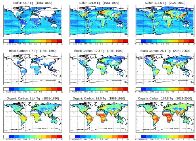
Sulfur: 44.7 Tg (1861-1890) 0 0.01 0.02 0.05 0.1 0.2 0.5 1 2 5 10 20 Sulfur: 101.9 Tg (1961-1990) 0 0.01 0.02 0.05 0.1 0.2 0.5 1 2 5 10 20 Sulfur: 116.6 Tg (2021-2050) 0 0.01 0.02 0.05 0.1 0.2 0.5 1 2 5 10 20 Black Carbon: 1.7 Tg (1861-1890) 0 0.005 0.01 0.02 0.05 0.1 0.2 0.5 1 2 5 10 Black Carbon: 12.3 Tg (1961-1990) 0 0.005 0.01 0.02 0.05 0.1 0.2 0.5 1 2 5 10 Black Carbon: 25.1 Tg (2021-2050) 0 0.005 0.01 0.02 0.05 0.1 0.2 0.5 1 2 5 10 Organic Carbon: 31.4 Tg (1861-1890) 0 0.005 0.01 0.02 0.05 0.1 0.2 0.5 1 2 5 10 Organic Carbon: 92.0 Tg (1961-1990) 0 0.005 0.01 0.02 0.05 0.1 0.2 0.5 1 2 5 10 Organic Carbon: 174.8 Tg (2021-2050) 0 0.005 0.01 0.02 0.05 0.1 0.2 0.5 1 2 5 10
Fig. 2. Global annual total 30-year average aerosol and precursor emissions for the periods 1861–1890, 1961–1990, and 2021–2050. Contours in g m−2yr−1.
the increased emission in the north-western Saharan source regions are a consequence of increased surface wind speeds. These changes of the regional climatological conditions can partly be attributed to an alteration of the monsoon regimes owing to an increase in atmospheric absorption due to in-creased carbonaceous emissions from vegetation fires (see R2006). It has to be pointed out that the dust emissions are calculated assuming fixed preferential source areas and year 2000 vegetation cover. Therefore, the simulated century scale variability is likely to be a lower estimate.
The evolution of the global distribution of the emissions of sulfur, black carbon, and particulate organic matter is il-lustrated in Fig. 2. Shown are the totals and distribution of the global annual aerosol and precursor emissions averaged over 30-year periods. It is clearly discernible that from the 1861–1890 to the 1961–1990 period the dominant emission increase took place at the east coast of the US, in Central Eu-rope and also in China. Contrary, from 1961–1990 to 2021– 2050 the US and European emissions are projected to de-crease and significant enhancements are expected in the low latitude regions South America, Central and South Africa, and South Asia.
3.2 Atmospheric aerosol burdens
The changes in the atmospheric emissions are reflected in the atmospheric aerosol column burdens, shown as totals and global distribution for sulfate, black carbon, and par-ticulate organic matter as 30-year averages for the periods 1861–1890, 1961–1990, and 2021–2050 in Fig. 3. Resem-bling the emission changes, the SU aerosol burden increases particularly in the northern hemispheric source regions from the 1861–1890 to the 1961–1990 period. With increasing emissions also the export from the sources regions increases, particularly from Europe to the Mediterranean and northern Africa. To the 2021–2050 period, the high latitude emissions are projected to decrease and high values of the burden are largely confined to low latitude regions. For BC and POM the contribution of the low-latitude emissions increases through-out the integration period. With decreasing high-latitude BC and POM emissions from 1961–1990 to 2021–2050, the low-latitude atmospheric aerosol burden is projected to dominate for the future conditions.
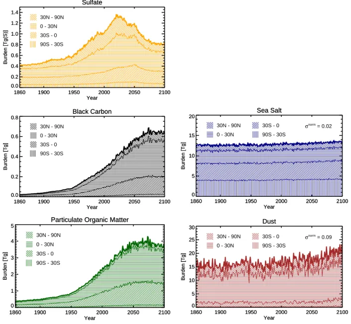
The temporal evolution of the atmospheric aerosol burden is shown as total and separated for four equal area latitude
Sulfate: 0.4 Tg(S) (1861-1890) 0 0.01 0.02 0.05 0.1 0.2 0.5 1 2 5 10 20 Sulfate: 0.9 Tg(S) (1961-1990) 0 0.01 0.02 0.05 0.1 0.2 0.5 1 2 5 10 20 Sulfate: 1.2 Tg(S) (2021-2050) 0 0.01 0.02 0.05 0.1 0.2 0.5 1 2 5 10 20 Black Carbon: 0.0 Tg (1861-1890) 0 0.01 0.02 0.05 0.1 0.2 0.5 1 2 5 10 20 Black Carbon: 0.2 Tg (1961-1990) 0 0.01 0.02 0.05 0.1 0.2 0.5 1 2 5 10 20 Black Carbon: 0.5 Tg (2021-2050) 0 0.01 0.02 0.05 0.1 0.2 0.5 1 2 5 10 20 POM: 0.4 Tg (1861-1890) 0 0.1 0.2 0.5 1 2 5 10 20 50 100 200 POM: 1.5 Tg (1961-1990) 0 0.1 0.2 0.5 1 2 5 10 20 50 100 200 POM: 3.5 Tg (2021-2050) 0 0.1 0.2 0.5 1 2 5 10 20 50 100 200
Fig. 3. Global total 30-year average aerosol burdens for the periods 1861–1890, 1961–1990, and 2021–2050. Contours in mg(S) m−2for SU and mg m−2for BC and POM.
bands in Fig. 4. As the aerosol residence-time is short, aerosols do not accumulate and the trends in the global an-nual mean aerosol burdens to a first order resemble the trends in the aerosol emissions with a peak of the SU aerosol burden centred around the year 2020, maximum values of POM bur-den around 2050, and a maximum of BC around 2070. Most prominently for BC and POM, but to a minor degree also for SU, the dominant aerosol increase occurs at low latitudes. This can be attributed to the fact that a significant part of the projected emission increase is from tropical vegetation fires and from increased fossil fuel usage in developing countries. For sea salt the total aerosol burden and meridional distribu-tion shows only minor variadistribu-tions. The increase in the dust burden, discernible from the year 2000 onwards, is most pro-nounced in the 0◦to 30◦N band owing to the northward shift of the African dust emissions described in the last section. 3.3 Atmospheric residence-times
As many greenhouse gases have long and approximately con-stant atmospheric residence-times, the discussion about pol-lutant mitigation is generally expressed in terms of emission scenarios, implicitly assuming that the atmospheric burden is
directly linked to the global total amount of emissions. For the short lived aerosols, however, the atmospheric residence-time (τ ) is not necessarily constant and depends on the residence-time and point of emission, chemical, thermodynamical and mi-crophysical transformations (“aging”), and on the meteoro-logical conditions along the aerosol trajectories (Graf et al., 1997; Barth and Church, 1999; Stier et al., 2006). Fig-ure 5 shows the evolution of the component residence-times throughout the integration period. It is clearly discernible that the residence-time shows non-negligible variations for all components. Changes in precipitation affect the aerosol residence time via the interactively calculated wet deposition rate. However, the general increase of the residence time from about 1950 onwards cannot be explained by the change in precipitation which actually increases by about 3% from 1860 to 2100 (not shown). The interpretation of this com-plex evolution of the atmospheric residence-times involves a number of competing processes and interactions.
For SU, τ decreases from about 4.5 days at pre-industrial times to about 4 days around 1950. Thereafter, in particu-lar with the distinct shift to low-latitude source regions af-ter 2025 and high burdens in the arid subtropical regions
Sulfate 1860 1900 1950 2000 2050 2100 Year 0.0 0.2 0.4 0.6 0.8 1.0 1.2 1.4 Burden [Tg(S)] Sulfate 1860 1900 1950 2000 2050 2100 Year 0.0 0.2 0.4 0.6 0.8 1.0 1.2 1.4 Burden [Tg(S)] 30N - 90N 0 - 30N 30S - 0 90S - 30S Black Carbon 1860 1900 1950 2000 2050 2100 Year 0.0 0.2 0.4 0.6 0.8 Burden [Tg] Black Carbon 1860 1900 1950 2000 2050 2100 Year 0.0 0.2 0.4 0.6 0.8 Burden [Tg] 30N - 90N 0 - 30N 30S - 0 90S - 30S Sea Salt 1860 1900 1950 2000 2050 2100 Year 0 5 10 15 20 Burden [Tg] σnorm = 0.02 Sea Salt 1860 1900 1950 2000 2050 2100 Year 0 5 10 15 20 Burden [Tg] 30N - 90N 0 - 30N 30S - 0 90S - 30S
Particulate Organic Matter
1860 1900 1950 2000 2050 2100 Year 0 1 2 3 4 5 Burden [Tg]
Particulate Organic Matter
1860 1900 1950 2000 2050 2100 Year 0 1 2 3 4 5 Burden [Tg] 30N - 90N 0 - 30N 30S - 0 90S - 30S Dust 1860 1900 1950 2000 2050 2100 Year 0 5 10 15 20 25 30 Burden [Tg] σnorm = 0.09 Dust 1860 1900 1950 2000 2050 2100 Year 0 5 10 15 20 25 30 Burden [Tg] 30N - 90N 0 - 30N 30S - 0 90S - 30S
Fig. 4. Global total atmospheric aerosol burdens from 1860–2100 (bold line) accumulated from bottom to top over the equal area latitude bands from 90◦S to 30◦S, from 30◦S to 0◦, from 0◦to 30◦N, and from 30◦N to 90◦N (hatched).
(Figs. 2, 3, 4), τ increases, reaching about 5.5 days around 2050, and remains relatively stable afterwards.
For BC, τ decreases from 6.5 days in 1860 to around 5 days in 1960 and increases thereafter to to 8 days in 2100. The initial decrease in the residence-time is contradictory to the increasing importance of low latitude dry-season vege-tation fire emissions (c.f. Figs. 2, 3). However, for the ini-tially emitted insoluble BC microphysical aging processes play an important role. From Fig. 6, depicting the evolu-tion of the microphysical aging-time, i.e. the timescale of transformation from the insoluble to the soluble modes (see Stier et al., 2005), it becomes evident that the BC aging-time is approximately halved from 1860 to 1950. As a conse-quence, the mass fraction of BC residing in the efficiently
scavenged internally-mixed accumulation mode soluble in-creases (Fig. 7), explaining the initial decrease in the BC residence-time. From about 1960 onwards, the increase in the residence-time indicates that the further enhanced aging to the peak of the sulfate burden in 2020 is outweighed by the shift to low latitude emissions, with a large contribution of dry-season vegetation fire emissions.
For POM, after a slow increase from about 4.5 days in 1860 to 5.5 days around 1960, τ increases more rapidly to 8.5 days in the year 2100, closely tracking the evolution for BC. This is a result of the increasing relative importance of the low-latitude dry-season vegetation fire emissions, from which BC and POM are co-emitted.
Residence Time 1860 1900 1950 2000 2050 2100 Year 3 4 5 6 7 8 9 SU BC POM DU [days] 0.60 0.65 0.70 0.75 0.80 0.85 0.90 SS [days] Sulfate Black Carbon Particulate Organic Matter Dust
Sea Salt
Fig. 5. Global mean atmospheric aerosol component residence time from 1860–2100.
Microphysical Aging Time
1860 1900 1950 2000 2050 2100 Year 0.0 0.5 1.0 1.5 2.0 2.5 3.0
BC and POM [days]
0.0 2.0 4.0 6.0 8.0 10.0 DU [days] Black Carbon Particulate Organic Matter Dust
Fig. 6. Global mean atmospheric microphysical component aging-time from 1860–2100.
Interestingly, the residence-time of SS also increases by about 6% from 1860 to 2100. Changes in the surface winds, with a poleward shift of the mid-latitude tropospheric wester-lies (see R2006) cause a poleward shift of the SS emissions. This shift is particularly pronounced in the southern latitudes. Associated is a small but continuous shift of the sinks from wet deposition to turbulent dry deposition and sedimentation (not shown). As the high latitude regions are dominated by ice clouds with a slightly reduced scavenging efficiency (c.f. Stier et al., 2005) this could explain the increase in the SS residence-time.
For DU, τ increases from 2000 to 2100 continuously from about 5 to 6 days. This is caused by the north-western shift of the dominant African sources into more arid regions and supported by an associated shift of the sinks from wet de-position to sedimentation. The enhanced microphysical ag-ing under more polluted conditions, indicated by decreased aging-times (Fig. 6) and the associated enhanced mass frac-tion in the soluble coarse mode (Fig. 7), that potentially re-duces τ appears to be a second order effect. Nonetheless, it could explain the relative stable residence-times from 1860 to 2000 and the enhanced increase after the peak of the sul-fate burden in 2020.
3.4 Aerosol mixing state
A number of aerosol parameters, such as the mixing state, are fixedly imposed in the mass based bulk modelling approach applied in traditional global aerosol models. However, the observed large internally-mixed aerosol population is a clear indicator that the mixing state is not constant for different levels of emissions and therefore not under different climatic regimes. The application of the microphysical aerosol mod-ule in a transient climate simulation allows to investigate the evolution of previously imposed parameters from prognostic variables.
The evolution of the global mean aerosol component mass partitioning among the seven aerosol modes of HAM (Ta-ble 1) from 1860–2100 is shown in Fig. 7. For the anthro-pogenically relevant species SU, BC, and POM it is evident that under the higher polluted conditions their mass shifts from the Aitken modes to the internally mixed accumulation mode soluble. This mode is of particular importance for the aerosol radiative effects. On the one hand, hydrophilic parti-cles in that size-range serve as cloud condensation nuclei and play therefore a key role for the indirect aerosol effects. On the other hand, it follows from Mie theory that particles in this size-range have the highest extinction efficiency for the visible wavelengths and therefore the strongest potential to contribute to the direct aerosol effects. For DU, a larger mass fraction is aged to the soluble modes under more polluted conditions, consistent with the evolution of the microphysi-cal aging-time shown in Fig. 6. The soluble mass fraction of DU decreases with the decay of the SU and POM burdens.
The disproportionate emission changes of the different aerosol components and precursors (Sect. 3.1) imply alter-ations of the composition of internally mixed modes. The simulated evolution of the composition of the internally mixed modes of HAM is displayed in Fig. 8. Sulfate is, with a relatively constant mass-fraction of 90%, the domi-nant component of the soluble Aitken mode from 1860 to around 2020. Thereafter, the sulfate fraction decreases to 80% in 2100 as the carbonaceous contribution increases. For the Aitken mode insoluble, the mass fraction of POM grad-ually decreases from 90% in 1860 to 70% in 2100, balanced by an increase in BC. This is largely a consequence of the in-creasing emission ratio of BC to POM. For the coarse mode soluble the mass fraction of DU increases from about 35% to 45% balanced by a decrease in sea salt, attributable to en-hanced microphysical aging of dust and a relative increase in the total DU burden.
The evolution of the radiatively important internally-mixed accumulation mode soluble is more complex. With the increase in the anthropogenic emissions, the contribu-tions of the natural components DU and SS are reduced from about 35% in 1860 to 10% in the year 2020. The in-crease in the sulfate mass is outweighed by the inin-crease in carbonaceous aerosols, particularly POM, so that the mass fraction of sulfate decreases constantly. This decrease is
Sulfate 1860 1900 1950 2000 2050 2100 Year 0 20 40 60 80 100 Massfraction [%] Nucleation Soluble Aitken Soluble Accumulation Soluble Coarse Soluble Aitken Insoluble Accumulation Insoluble Coarse Insoluble Dust 1860 1900 1950 2000 2050 2100 Year 0 20 40 60 80 100 Massfraction [%] Nucleation Soluble Aitken Soluble Accumulation Soluble Coarse Soluble Aitken Insoluble Accumulation Insoluble Coarse Insoluble Black Carbon 1860 1900 1950 2000 2050 2100 Year 0 20 40 60 80 100 Massfraction [%] Nucleation Soluble Aitken Soluble Accumulation Soluble Coarse Soluble Aitken Insoluble Accumulation Insoluble Coarse Insoluble
Particulate Organic Matter
1860 1900 1950 2000 2050 2100 Year 0 20 40 60 80 100 Massfraction [%] Nucleation Soluble Aitken Soluble Accumulation Soluble Coarse Soluble Aitken Insoluble Accumulation Insoluble Coarse Insoluble
Fig. 7. Global mean aerosol component partitioning among the seven aerosol modes of HAM from 1860–2100.
enhanced after the sulfate peak in the year 2020 so that POM becomes the dominant component in the accumulation mode soluble after 2050. The mass fraction of BC increases con-stantly from 0% in 1860 to around 7% in 2100.
3.5 Aerosol radiative properties and perturbations
These changes in the composition of the internally mixed modes, with a relative increase in the carbonaceous aerosols, have distinct effects on their interactively calculated radia-tive properties. Here we focus on the internally-mixed ac-cumulation mode soluble as it dominates the anthropogenic contribution to the aerosol radiative effects. The effect of the increasing importance of the carbonaceous aerosols is nicely demonstrated by the evolution of the global mean op-tical depth weighted co-single scattering albedo (CO-SSA) at a wavelength of 550 nm depicted in Fig. 9. The CO-SSA, as a measure of the contribution of absorption to the total ex-tinction, increases constantly from 0.02 in 1860 to 0.04 in 2020. This is a consequence of the increase in the carbona-ceous mass fraction, particularly of BC, with higher imag-inary parts of the refractive indices (see Stier et al., 2005). With the decline of the projected sulfate emissions in 2020 the increase in the CO-SSA is further enhanced, reaching a plateau of more than 0.07 in the year 2070.
In summary, the projected changes in the aerosol emis-sions distinctively affect the aerosol mixing state and the
composition of the internally mixed modes on the global scale. Consequently, their radiative properties are altered with a significant enhancement of the absorption efficiency, owing to the increased contribution of carbonaceous aerosols throughout the integration period.
Changes in the atmospheric aerosol burden and composi-tion affect the aerosol optical depth (AOD), i.e. the column integrated aerosol extinction. The evolution of the global mean total tropospheric aerosol optical depth, fine mode op-tical depth (Aitken and accumulation modes), coarse mode optical depth, and the absorption optical depth at 550 nm is shown in Fig. 11. Total AOD increases from a pre-industrial level of 0.15 to 0.26 in year 2020. The decrease in the SU contribution after 2020 is partly compensated by the increase in POM so that AOD decreases only weakly and levels off to 0.23 in the year 2100. It is interesting to note that the domi-nant increase in total AOD can be attributed to an increase in the fine mode AOD confirming the assumption that anthro-pogenic aerosols predominantly affect the fine mode aerosol optical depth. However, these results do not support the re-verse, i.e. that the fine mode optical depth is a direct measure of the anthropogenic aerosol radiative effects. In fact, more than a third of the simulated fine mode optical depth for the year 2000 is of natural origin, indicated by the values at the beginning of the integration period. The natural fine mode optical depth is dominated by volcanic sulfate but shows also
contributions from DMS derived sulfate, biogenic POM, as well as from sub-micron sea salt and mineral dust.
In Fig. 10 the simulated 1998-2002 mean aerosol optical depth is compared on a regional basis to five different mea-surement datasets: to a retrieval from the AERONET sun-photometer network (Holben et al., 2001) extrapolated and gridded on a 1◦×1◦resolution (1998–2004 mean of available measurements, S. Kinne, personal communication, 2006), as well as to satellite retrievals from MODIS (2000-2004 mean, Tanr´e et al., 1997; Kaufman et al., 1997), MISR (2000– 2004 mean, Martonchik et al., 2002, 2004), AVHRR (2001 mean, Ignatov and Stowe, 2002a,b), and TOMS (1996–2000 mean, Torres et al., 2002). For comparison, results from the Stier et al. (2005) year 2000 reference simulation with ECHAM5–HAM are provided, utilising the AeroCom emis-sion inventory. At large, the regional distribution of the ob-served AOD is well captured in the MPI–ESM simulation. The global 1998–2002 mean AOD of 0.22 is somewhat larger than the global 2000–2004 mean AODs from MODIS (0.20) and MISR (0.21), that provide probably the highest quality datasets with global coverage. However, this good agreement on a global mean basis should be regarded with the caveat that the satellite retrievals exhibit non-negligible uncertain-ties and both the MODIS and MISR retrievals are likely to be biased high (Levy et al., 2005; Liu et al., 2004). On a regional basis, the overestimation of AODs is particularly pronounced in the Saharan dust outflow region but also in the main an-thropogenic source regions, China, Europe, and the eastern United States. It is not possible to quantitatively attribute this overestimation to specific causes, but the comparison to the ECHAM5–HAM reference simulation (global annual mean AOD of 0.14) can give further insight. Higher emissions of mineral dust, of about 1200 Tg yr−1around year 2000 in the
free climate mode compared to emissions of about about 670 Tg yr−1in the nudging mode applied in the reference simula-tion, contribute to the overestimation of AOD in the Saharan outflow region. These higher emissions are a consequence of a shift of the surface wind speed frequency distribution to higher wind speeds in the climate mode. See Timmreck and Schulz (2004) for more details. Stronger anthropogenic emissions in the NIES emission inventory compared to the AeroCom inventory contribute to the overestimation of the aerosol optical depths close to the main anthropogenic source regions compared to both the remote sensing data and the ref-erence simulation.
The evolution of the absorption aerosol optical depth (AAOD), i.e. the column integrated aerosol extinction ow-ing to absorption (Fig. 11), shows a distinct increase from pre-industrial levels of around 0.001 and levels off around 0.01 in the year 2070. This increase is dominated by the in-crease in the fine mode AAOD attributable to the inin-crease in the total BC burden (linear Pearson’s correlation coefficient
r=0.999). The small increase in coarse mode AAOD can be attributed to the increase in the DU burden (r=0.995).
The development of the aerosol distribution and radiative properties determines their direct effects on the global radi-ation balance. Figure 12 shows the evolution of the simu-lated global mean total aerosol short-wave clear-sky direct radiative perturbation (DARP), together with the prescribed aerosol optical depth owing to volcanic aerosols in the strato-sphere. DARP is defined here as the deviation of the clear-sky net short wave radiation at the top of the atmosphere from the 1860–1870 mean. DARP is calculated as the change in the clear-sky net top-of-the-atmosphere solar radiation, cor-rected for variations in the top-of-the-atmosphere solar irra-diance and for the associated change in the upward surface radiation. The correction for the change in the upward sur-face radiation from the stored model variables requires the assumption of constant surface albedos. Therefore, areas with a change in surface albedo larger than 0.03 as well as sea-ice covered regions are masked out. The masked areas constitute generally less than 14% of the earth’s surface.
Superimposed to the anthropogenic trends are distinct DARPs from volcanic eruptions, reaching values of around
−4 Wm−2 for the major Krakatoa (1883) and Mount
Pinatubo (1991) eruptions. With increasing anthropogenic AOD, the negative DARP intensifies, reaches −0.8 Wm−2 around 2000, peaks with about −1.1 Wm−2around 2020 and remains relatively stable up to 2050, largely because the con-tinued increase in POM outweighs the decrease in SU after 2020. Although AOD remains at a higher level than in 2000 thereafter, DARP weakens, reaching −0.6 Wm−2 in 2100. This can be attributed to an increase in atmospheric absorp-tion owing to the BC increase (Fig. 11). It is interesting to note that the combination of volcanic and anthropogenic aerosol perturbations between about 1950 and 1970 causes a distinct negative DARP of up to −2 Wm−2. This negative radiative perturbation contributes to mask out the effect of increased greenhouse gas emissions on the global tempera-ture. In combination with the stagnation and even reversal of the increase of the solar irradiance after about 1930–1940 (Solanki and Krivova, 2003; Krivova and Solanki, 2004), this explains the well simulated small trend in global surface tem-peratures between 1950 and 1970 (see Fig. 1 in R2006) de-spite the increasing positive greenhouse gas forcing (see also discussion in McAvaney et al., 2001).
4 Conclusions
The evolution of the global aerosol system from 1860 to 2100 is investigated through a transient atmosphere-ocean GCM climate simulation with interactively coupled atmospheric aerosol and oceanic biogeochemistry modules. The micro-physical aerosol module HAM incorporates the major global aerosol components sulfate, black carbon, particulate organic matter, sea salt, and mineral dust with prognostic treatment of their composition, size distribution, and mixing state.
Aitken Soluble 1860 1900 1950 2000 2050 2100 Year 0 20 40 60 80 100 Massfraction [%] Sulfate Black Carbon Particulate Organic Matter Sea Salt Dust Aitken Insoluble 1860 1900 1950 2000 2050 2100 Year 0 20 40 60 80 100 Massfraction [%] Sulfate Black Carbon Particulate Organic Matter Sea Salt Dust Accumulation Soluble 1860 1900 1950 2000 2050 2100 Year 0 20 40 60 80 100 Massfraction [%] Sulfate Black Carbon Particulate Organic Matter Sea Salt Dust Coarse Soluble 1860 1900 1950 2000 2050 2100 Year 0 20 40 60 80 100 Massfraction [%] Sulfate Black Carbon Particulate Organic Matter Sea Salt
Dust
Fig. 8. Global mean aerosol composition of the internally mixed aerosol modes of HAM from 1860–2100.
The atmosphere and ocean GCMs are coupled interac-tively, employing no flux correction. In addition, also the atmospheric and oceanic biogeochemical cycles are coupled interactively by accounting for the deposition of mineral dust acting as micro-nutrient for a prognostic ocean biogeochem-istry scheme and by emitting biogeochemically produced DMS from the ocean surface to the atmosphere. Also the natural emissions of mineral dust and sea salt are calculated interactively. Anthropogenic aerosol and precursor emis-sions are prescribed based on the Japanese National Institute for Environmental Studies emission inventory from 1860 to 2100. From pre-industrial to present day times greenhouse gases, volcanic stratospheric AOD, and solar variability are prescribed according to observations. For the 2000 to 2100 period, greenhouse gas concentrations as well as aerosol and precursor emissions are based on the SRES A1B scenario.
From pre-industrial times to 2020 the global mean sul-fate aerosol burden is projected to increase from 0.4 Tg(S) to 1.3 Tg(S) and thereafter to decrease to 0.8 Tg(S) in 2100. Aerosol burdens of BC and POM are increasing up to around 2070 peaking with burdens of 0.7 Tg and 4 Tg and show a small decrease thereafter. The burdens of natural sea salt and mineral dust also increase, however at a significantly slower rate. It has to be pointed out that the dust emissions are cal-culated assuming fixed preferential source areas and vegeta-tion cover. Natural secondary organics are prescribed at their year 2000 levels. Thus, the simulated variability and trends
CO-SSA - Accumulation Soluble
1860 1900 1950 2000 2050 2100 Year 0.00 0.02 0.04 0.06 0.08 0.10
Co-Single Scattering Albedo [1]
Fig. 9. Global mean optical depth weighted accumulation mode soluble co-single scattering albedo at 550 nm from 1860–2100.
of mineral dust and natural secondary organics potentially represent a lower estimate owing to the neglect of land-use and vegetation changes.
Regionally, the prognosed emissions and consequently the simulated aerosol burden show inhomogeneous trends. From present day to future conditions the anthropogenic aerosol burden shifts generally from the northern high-latitudes to the developing low-latitude source regions. The resulting spatially inhomogeneous radiative perturbations are a driv-ing force for regional climate change.
MPI-ESM AERONET MODIS MISR TOMS AVHRR ECHAM5-HAM AOD(550nm) 0.1 0.2 0.3 0.4
Fig. 10. Regional comparison of simulated aerosol optical depth at 550 nm (red, 1998–2002 mean) to retrievals from the AERONET sun-photometer (yellow, 1998–2004 mean of available measurements), and from the satellite instruments MODIS (dark blue, 2000–2004 mean), MISR (light blue, 2000–2004 mean), TOMS (dark green, 1996–2000 mean), and AVHRR (light green, 2001 mean). Grey shading indicates the averaging areas. For comparison, results from the Stier et al. (2005) year 2000 reference simulation with ECHAM5-HAM, employing the AeroCom emission inventory, are given (orange).
The projected increase in low-latitude carbonaceous aerosols and the associated increase in the atmospheric ab-sorption cause an enhancement of local monsoon regimes, particularly pronounced over Central Africa (see R2006). The associated changes in the flow pattern and the increase in precipitation and soil moisture shifts emission regimes and the atmospheric burden of mineral dust northward. Such cou-plings of the global aerosol cycles, acting in addition to the coupling by microphysical processes (Stier et al., 2006), will be further enhanced when climate-vegetation feedbacks are taken into account.
An analysis of atmospheric residence-times reveals signif-icant alterations under varying climatic and pollution con-dition during the integration period. Thus, the atmospheric aerosol burden and therefore the aerosol radiative effects can-not be scaled by global annual mean emission data. The evo-lution of the aerosol burden is rather the result of complex in-teractions of aerosol microphysics, formation pathways, the point of emission, and the meteorological conditions along the aerosol trajectories. For example, a given sulfate radia-tive perturbation in the year 2000, scaled to the year 2100 by the change of SO2emissions, would be biased low by a
fac-tor of τ2000/τ2100=4.3 days/5.6 days= 0.8 solely due to the neglect of the longer residence-time in 2100 (assuming con-stant sulfate yield from SO2emissions and constant aerosol
radiative properties).
In previous climate simulations, the microphysical aging-time of BC, POM, and DU, if considered, has been pre-scribed as constant. Here we show that it varies by as much as a factor of two during the integration, with enhanced aging under polluted conditions, peaking around the year 2020.
The projected inhomogeneous changes in the aerosol and precursor emissions distinctively affect the aerosol mixing state and the composition of the internally mixed modes. With increasing levels of anthropogenic pollution, the frac-tion of SU, BC, and POM residing in the radiatively impor-tant internally mixed accumulation mode increases, owing to enhanced microphysical interactions. Under the predicted emission changes, the global mean composition of the inter-nally mixed accumulation mode is altered with a steady in-crease in the contribution of carbonaceous aerosols. These composition changes are reflected in the aerosol radiative properties. The increasing fraction of carbonaceous aerosols in the internally-mixed accumulation mode causes a more than threefold increase in its co-single scattering albedo from 1860 to 2100. These findings are in contradiction to the tra-ditional approach of assuming constant radiative properties for each internally mixed mode. They further indicate that the aerosol radiative effects are altered by microphysical in-teractions of the different aerosol cycles.
The simulated global annual mean AOD at 550 nm in-creases from 0.15 at pre-industrial times to 0.22 around the year 2000. The present day values are somewhat larger than satellite retrieved estimates of MODIS (2000–2004 global mean of 0.20) and MISR (2000–2004 global mean of 0.21). However, it has been shown that these satellite retrievals ex-hibit a positive bias on a local basis. The simulated values are also higher than a year 2000 reference simulation with ECHAM5–HAM that shows a better agreement with the re-mote sensing data on a regional basis. This overestimation can be attributed to stronger mineral dust emissions in the free climate mode compared to the nudged reference simu-lation as well as to stronger anthropogenic emissions in the
Aerosol Optical Depths 1860 1900 1950 2000 2050 2100 Year 0.00 0.05 0.10 0.15 0.20 0.25 0.30 AOD [1] 0.000 0.002 0.004 0.006 0.008 0.010 Absorption AOD [1] AOD AOD fine AOD coarse Abs-AOD Abs-AOD fine Abs-AOD coarse
Fig. 11. Global mean total tropospheric aerosol optical depth (red) and absorption optical depth (black) at 550 nm from 1860–2100. Also given are fine mode (dashed) and coarse mode (dotted) values.
NIES emission compilation compared to the AeroCom emis-sion inventory applied in the reference simulation. From present day conditions to the pollution peak around 2020, AOD is projected to increase to 0.26. Despite the signifi-cant reduction of sulfate thereafter, AOD shows only a weak decrease as the continuing increase in carbonaceous aerosol is compensating. The anthropogenic enhancement of AOD is attributable to an increase in fine mode AOD. However, more than a third of the simulated global mean fine mode optical depth of the year 2000 is already present under natural con-ditions, contradicting the assumption that all fine mode AOD is attributable to anthropogenic activities. This introduces a significant uncertainty to remote sensing derived estimates of the anthropogenic contribution to the aerosol radiative effects (e.g. Christopher and Zhang, 2004; Kaufman et al., 2005). An integrated approach is required, combining the strengths of remote sensing and global modelling, to reduce the re-maining large uncertainties.
The simulated anthropogenic top of the atmosphere clear-sky short-wave direct aerosol radiative perturbation intensi-fies from pre-industrial times, reaching about −1.1 Wm−2 around 2020. Although AOD remains at a relative high level after 2050, DARP weakens to −0.6 Wm−2, attributable to an increase in atmospheric absorption owing to the continued increase in the BC burden. The onset of the anthropogenic negative DARP in combination with increasing volcanic ac-tivity between about 1950 and 1970 contribute to the well simulated observed small trend in global surface tempera-tures during that period, despite increasing greenhouse gas forcing.
To recapitulate, our results from a transient coupled AOGCM climate simulation from 1860 to 2100 with an em-bedded microphysical aerosol module show distinct alter-ations of the aerosol system on global and regional scales over the integration period. Aerosol residence-times, aging-times, size, composition, and mixing state undergo non-negligible variations. As a consequence, their radiative
prop-Direct Aerosol Radiative Perturbation
1860 1900 1950 2000 2050 2100 Year 0 -2 -4 -6 DARP [Wm -2] 0.0 0.1 0.2 0.0 0.0 Stratospheric AOD [1] 0.0 0.1 0.2 0.0 0.0 Stratospheric AOD [1]
Direct Aerosol Radiative Perturbation
1860 1900 1950 2000 2050 2100 Year 0 -2 -4 -6 DARP [Wm -2] DARP AOD
Fig. 12. Global mean total aerosol short-wave clear-sky direct ra-diative perturbation (red) and stratospheric volcanic aerosol optical depth at 550 nm (black, dashed) from 1860–2100 with respect to the 1860–1870 mean.
erties and effects and ultimately their climatic impact can-not be estimated solely based on changes of the global mean emissions.
Large uncertainties, in particular with respect to the future evolution of the aerosol system remain. Aerosol emission in-ventories even for present day conditions, based on largely well determined fuel use data, are highly uncertain, particu-larly for the carbonaceous compounds. These uncertainties propagate into the future emission scenarios and add to their large uncertainties regarding economic, population, techno-logical, and legislative developments. So one key outcome of this study are the demonstrated modifications of aerosol parameters that have previously been assumed constant – un-der one possible realisation of greenhouse gas, aerosol, and aerosol precursor emissions. Additional feedbacks of the aerosol cycles with other compartments of the earth system, such as aerosol effects on vegetation via fertilisation and so-lar dimming, the effect of changing vegetation on the surface emissions of dust and organic matter, as well as feedbacks with the atmospheric chemistry are also likely to affect the evolution of the aerosol system and will be subject of future research activities.
Acknowledgements. This research was supported by the German
Ministry for Education and Research (BMBF) under the DEKLIM Project and by the European Community under the ENSEMBLES Project. The simulations were performed on the NEC SX-6 su-percomputer of the German High Performance Computing Centre for Climate- and Earth System Research in Hamburg. We would like to thank T. Nozawa (National Institute for Environmental Studies, Japan) and T. Takemura (Kyushu University, Japan) for providing the aerosol emission dataset and their support. Many thanks to S. Kinne who helped with the AOD evaluation and internally reviewed the manuscript together with D. Banse. We would also like to thank I. Fischer-Bruns for helpful discussions and M. Werner (MPI-Biogeochemistry, Jena) for his support with the dust source. The continuous support of our colleagues L. Kornblueh, U. Schulzweida, U. Schlese, and R. Brokopf was greatly appreciated.
Edited by: S. Martin
References
Adams, P. J., Seinfeld, J. H., and Koch, D. M.: Global concen-trations of tropospheric sulfate, nitrate, and ammonium aerosol simulated in a general circulation model, J. Geophys. Res., 104, 13 791–13 824, 1999.
Albrecht, B. A.: Aerosols, cloud microphysics, and fractional cloudiness, Science, 245, 1227–1230, 1989.
Andreae, M. O.: Global biomass burning: Atmosphere, climatic, and biospheric implications, chap. Biomass burning: Its history, use and distribution, and its impact on environmental quality in global climate, 15–42, MIT Press, Cambridge, MA, 1991. ˚
Angstr¨om, A.: Atmospheric turbidity, global illumination and plan-etary albedo of the earth, Tellus, 14, 435–450, 1962.
Barth, M. C. and Church, A. T.: Regional and global distri-butions and lifetimes of sulfate aerosols from Mexico City and southeast China, J. Geophys. Res., 104, 30 231–30 240, doi:10.1029/1999JD900 809, 1999.
Christopher, S. A. and Zhang, J.: Cloud-free shortwave aerosol radiative effect over oceans: Strategies for identifying anthro-pogenic forcing from Terra satellite measurements, Geophys. Res. Lett., 31, L18 101, doi:10.1029/2004GL020 510, 2004. Cooke, W. F., Koffi, B., and Gregoire, J.-M.: Seasonality of
vege-tation fires in Africa from remote sensing data and application to a global chemistry model, J. Geophys. Res., 101, 21 051–21 065, 1996.
Cooke, W. F., Liousse, C., Cachier, H., and Feichter, J.: Con-struction of a 1◦×1◦fossil fuel emission data set for carbona-ceous aerosol and implementation and radiative impact in the ECHAM4 model, J. Geophys. Res., 104, 22 137–22 162, 1999. Dentener, F., Kinne, S., Bond, T., Boucher, O., Cofala, J., Generoso,
S., Ginoux, P., Gong, S., Hoelzemann, J. J., Ito, A., Marelli, L., Penner, J. E., Putaud, J.-P., Textor, C., Schulz, M., van der Werf, G. R., and Wilson, J.: Emissions of primary aerosol and precur-sor gases in the years 2000 and 1750, prescribed data-sets for AeroCom, Atmos. Chem. Phys. Discuss., 6, 2703–2763, 2006, http://www.atmos-chem-phys-discuss.net/6/2703/2006/. Feichter, J., Kjellstr¨om, E., Rodhe, H., Dentener, F., Lelieveld, J.,
and Roelofs, G.-J.: Simulation of the tropospheric sulfur cycle in a global climate model, Atmos. Environ., 30, 1693–1707, 1996. Fouquart, Y. and Bonnel, B.: Computations of solar heating of the
earth’s atmosphere: A new parameterization, Beitr. Phys. At-mos., 53, 35–62, 1980.
Graf, H.-F., Feichter, J., and Langmann, B.: Volcanic sulfur emis-sions: Estimates of source strength and its contribution to the global sulfate distribution, J. Geophys. Res., 102, 10 727–10 738, 1997.
Graßl, H.: Albedo reduction and radiative heating of clouds by absorbing aerosol particles, Contributions Atmospheric Physics, 48, 199–210, 1975.
Guenther, A., Hewitt, C. N., Erickson, D., Fall, R., Geron, C., Graedel, T., Harley, P., Klinger, L., Lerdau, M., McKay, W. A., Pierce, T., Scholes, B., Steinbrecher, R., Tallamraju, R., Taylor, J., and Zimmerman, P.: A global model of natural volatile or-ganic compound emissions, J. Geophys. Res., 100, 8873–8892, 1995.
Hansen, J., Nazarenko, L., Ruedy, R., Sato, M., Willis, J., Genio, A. D., Koch, D., Lacis, A., Lo, K., Menon, S., Novakov, T., Perlwitz, J., Russell, G., Schmidt, G. A., and Tausnev, N.: Earth’s energy imbalance: confirmation and implications, Science, 308, 1431–1435, doi:10.1126/science.1110252, 2005.
Hansen, J., Sato, M., and Ruedy, R.: Radiative forcing and climate response, J. Geophys. Res., 102, 6831–6864, 1997.
Holben, B. N., Tanr´e, D., Smirnov, A., Eck, T. F., Slutsker, I., Abuhassan, N., Newcomb, W. W., Schafer, J. S., Chatenet, B., Lavenu, F., Kaufman, Y. J., Castle, J. V., Setzer, A., Markham, B., Frouin, D. C. R., Halthore, R., Karneli, A., O’Neill, N. T., Pietras, C., Pinker, R. T., Voss, K., and Zibordi, G.: An emerging ground-based aerosol climatology: Aerosol optical depth from AERONET, J. Geophys. Res., 106, 12 067–12 098, 2001. Ignatov, A. and Stowe, L.: Aerosol retrievals from individual
AVHRR channels. part I: retrieval algorithm and transition from dave to 6S radiative transfer model, J. Atmos. Sci., 59, 313–334, 2002a.
Ignatov, A. and Stowe, L.: Aerosol retrievals from individual AVHRR channels. part II: quality control, probability distribu-tion funcdistribu-tions, informadistribu-tion content, and consistency checks of retrievals, J. Atmos. Sci., 59, 335–362, 2002b.
Ito, A. and Penner, J. E.: Historical emissions of carbonaceous aerosols from biomass and fossil fuel burning for the pe-riod 1870–2000, Global Biogeochem. Cycles, 19, GB2028, doi:10.1029/2004GB002 374, 2005.
Jacobson, M. Z.: Control of fossil-fuel particulate black car-bon and organic matter, possibly the most effective method of slowing global warming, J. Geophys. Res., 107, 4410, doi:10.1029/2001JD001 376, 2002.
Johns, T. C., Gregory, J. M., Ingram, W. J., Johnson, C. E., Jones, A., Lowe, J. A., Mitchell, J. F. B., Roberts, D. L., Sexton, D. M. H., Stevenson, D. S., Tett, S. F. B., and Woodage, M. J.: An-thropogenic climate change for 1860 to 2100 simulated with the HadCM3 model under updated emissions scenarios, Clim. Dyn., 20, 583–612, doi:10.1007/s00382-002-0296-y, 2003.
Johnson, K., Gordon, R., and Coale, K.: What controls dissolved iron concentrations in the world ocean?, Marine Chemistry, 57, 137–161, 1997.
Jungclaus, J., Botzet, M., Haak, H., Keenlyside, N., Luo, J., Latif, M., Marotzke, J., Mikolajewicz, U., and Roeckner, E.: Ocean circulation and tropical variability in the coupled model ECHAM5/MPI-OM, J. Clim., in press, 2006.
Kaufman, Y. J., Tanr´e, D., Remer, L. A., Vermote, E. F., Chu, A., and Holben, B. N.: Operational remote sensing of tropospheric aerosol over land from EOS moderate resolution imaging spec-troradiometer, J. Geophys. Res., 102, 17 051–17 068, 1997. Kaufman, Y. J., Boucher, O., Tanr´e, D., Chin, M., Remer, L. A.,
and Takemura, T.: Aerosol anthropogenic component esti-mated from satellite data, Geophys. Res. Lett., 32, L17 804, doi:10.1029/2005GL023 125, 2005.
Khairoutdinov, M. and Kogan, Y.: A new cloud physics parameter-ization in a Large-Eddy simulation model of marine stratocumu-lus, Mon. Wea. Rev., 128, 229–243, 2000.
Kloster, S., Feichter, J., Maier-Reimer, E., Six, K., Stier, P., and Wetzel, P.: DMS cycle in the marine oceanatmosphere system -a glob-al model study, Biogeosci., 3, 29–51, 2006.
Krivova, N. and Solanki, S.: Solar variability and global warming: a statistical comparison since 1850, Adv. Space Res., 34, 361–364,