Design of feedback control systems for unstable plants with saturating actuators

July 1988 LIDS-P-1838 Design of Feedback Control Systems for Unstable Plants

with Saturating Actuators' by

Petros Kapasouris * Michael Athans Gunter Stein **

Room 35-406

Laboratory for Information and Decision Systems Massachusetts Institute of Technology

Cambridge, MA 02139

Key Words - Automatic Control Systems, Nonlinear Control, Multivariable Control.

ABSTRACT

A new control design methodology is introduced for multi-input/multi-output systems with unstable open loop plants and saturating actuators. A control system is designed using well known linear control theory techniques and then a reference prefilter is introduced so that when the references are sufficiently small, the control system operates linearly as designed. For signals large enough to cause saturations, the control law is modified in such a way to ensure stability and to preserve, to the extent possible, the behavior of the linear control design.

Key benefits of this methodology are: the modified feedback system never produces saturating control signals, integrators and/or slow dynamics in the compensator never windup, the directional properties of the controls are maintained, and the closed loop system has certain guaranteed stability properties.

The advantages of the new design methodology are illustrated in the simulation of an approximation of the AFTI-16 (Advanced Fighter Technology Integration) aircraft multivariable longitudinal dynamics.

1

This research was conducted at the M.I.T. Laboratory for Information and Decision Systems with support provided by the General Electric Corporate Research and Development Center, and by the NASA Ames and Langley Research Centers under grant

NASA/NAG 2-297.

* Now with ALPHATECH Inc. ** Also with HONEYWELL Inc.

Page 1

1. Introduction

In general the presence of saturations introduce stability and performance problem to closed loop multivarible control systems. One of those problems is the fact that control saturations alter the direction of the control vector. Each saturation element operates on its input signal

independently of the other saturation elements; as it has been shown in the performance analysis in [10] and [11] this can disturb the direction of the applied control vector. Consequently, erroneous controls can occur causing degradation of the performance of the closed loop system over and above the expected fact that output transients will be "slower".

Another performance degradation occurs when a linear compensator with integrators is used in a closed loop system and the phenomenon of reset-windup appears. During the time of

saturation of the actuators, the error is continuously integrated even though the controls are not what they should be. The integrator, and other slow compensator states, attain values that lead to larger controls than the saturation limits. This leads to the phenomenon known as reset-windup, resulting in serious deterioration of the performance (large overshoots and large settling times.).

The effects of the saturations on the closed loop stability of the control system are well known. When the open loop plant is unstable one can only guarantee local closed loop 'stability and there are references and disturbances such that when applied the closed loop system becomes unstable.

Many attempts have been made to address these problems for SISO systems, but a general design process has not been formalized. One way to design controllers for systems with bounded controls, would be to solve an optimal control problem; for example, the time optimal control problem or the minimum energy problem etc. The solution to such problems usually leads to a bang-bang feedback controller [1]. Even though the problem has been solved completely in

principle, the solution to even the simplest systems requires good modelling, is difficult to calculate open loop solutions, or the resulting switching surfaces are complicated to work with. For these reasons, in most applications the optimal control solution is not used.

Because of the problems with optimal control results, other design techniques have been attempted. Most of them are based on solving the Lyapunov equation and getting a feedback which

Page 2

will guarantee global stability when possible or local stability otherwise [2]-[3]. The problem with these techniques is that the solutions tend to be unnecessarily conservative and consequently the performance of the closed loop system may suffer.

Attempts to solve the reset windup problems when integrators are present in the forward loop, have been made for SISO systems [4]-[6]. Most of these attempts lead to controllers with substantially improved performance but not well understood stability properties. As part of this research, an initial investigation was made on the effects on performance of the reset windups for MIMO systems [8] showing potential for improving the performance of the system. A simple case study was also recently conducted on the effects of saturations to MIMO systems where potential for improvement in the performance was demonstrated [9].

A new design methodology has been introduced in [11] for designing MIMO control systems for stable open loop plants with multiple saturations. Here a systematic methodology is

introduced to design control systems with multiple saturations for unstable open loop plants. The idea is to design a linear control system ignoring the saturations and when necessary to modify that linear control law. When the exogenous signals are small, and they do not cause saturations, the system operates linearly as designed. When the signals are large enough to cause saturations, the references are modified in such a way to preserve ("mimic") to the extent possible the responses of the linear design. Our modification to the linear compensator is introduced at the error via a

Reference Governor (RG).

2. Performance Analysis

Without loss of generality one can assume that each element ui (t) of the control vector u(t) = [ ul(t) ... up(t)]T has saturation limits +1 and the saturation operator can be defined as follows:

1 ui( t )> 1

sat(u))= ui(t) -1 u.(t) 1 (2.1)

Page 3

Figure 2.1 shows the closed loop system with the saturation element f(u(t)) (f(u(t)) = [sat(ul(t) .. .sat(um(t)]T) at the controls. The compensator K(s) is designed using linear control system techniques and it is assumed that the closed loop system without the saturations (the linear system) is stable with "good" properties.

d i(t) do (t)

K(s)

f(u(t))

G(s)

refeec errorence + + output

Compensator Saturation Plant

Figure 2.1: The closed loop system

There are well developed methods for defining performance criteria and for designing linear closed loop systems which meet the performance requirements. It would then be desirable, whenever the closed loop system operates in the linear region, to meet the a priori performance constraints (because it easy to define them and easy to design control systems satisfying these constraints). When the system operates in the nonlinear region new performance criteria have to be defined and new ways of achieving the desired performance must be developed.

There are two major problems that multiple saturations can introduce to the performance of the system: (a) the reset windup problem, and (b) the fact that multiple saturations change the direction of the controls.

When the linear compensator contains integrators and/or slow dynamics reset windups can occur. It is obvious that if the states of the compensator were such that the controls would never saturate, then reset windups would never appear. More information about the performance degradation of the feedback system caused by the saturations is given in [12].

To solve the performance problem a nonzero operator 02 is applied in the reference signals and it will be called Reference Governor (RG).

Page 4 The nonzero operator is chosen, if possible, so that the control u(t) never saturates, i.e. Ilu(t)11io < 1, for any reference and/or disturbances. It is also desired that the 02r signals are "close" to the r(t) signals. In section 4 the RG operator will be defined in detail.

3. Mathematical preliminaries

This section is an introduction to the new design methodology. Some necessary mathematical preliminaries will be given and a basic problem will be introduced. The basic problem will be solved and it's solution will lead to the new control design methodology.

Consider the following linear time invariant system

x(t) = Ax(t), x(O) = x AE Rnx n, x(t) E Rn (3.1) mxn

y(t) = Cx(t) C E R x _{, y(t) E}

RIm (3.2)

y(xo,t) = Ce Axo _(3.3)

where eAt is the state transition matrix (matrix exponential) for A

Definition 3.1: The scalar-valued function g(x) is defined as follows:

g(xo): R -'-> R, g(xo) = LY(xo,t)ll (3.4)

Definition 3.2: The set Pg is defined as:

Pg =

t

Definition 3.3: BA,C is the set of all xE iRn with 0 < g(x) < 1, i.e.

BA,C =f X: 0 < g(x)1} (3.6)

Suppose that the system (3.1)-(3.3) has an initial condition xo0 BA,C. From this definition we see that for such an initial condition the output of the system, y(t), will satisfy liy(t)11,, < 1. For neutrally stable systems the function g(x), the set Pg and the set BA,c have the following

properties.

(a) The set Pg is a convex cone.

(b) The BA,C set is symmetric with respect to the origin and convex. (c) .The function g(x) is continuous and even.

Page 5

Definition 3.4 [71: The upper right Dini derivative is defined as

D f(to) = lim sup f(t)(3.7)

t_)to t-to

The D+f(to) is finite at to if the function f satisfies the Lipschitz condition locally around to [7]. Note that the function g(x) defined by Definition 3.1 satisfies the Lipschitz condition locally if and only if the system (3.1)-(3.3) is neutrally stable.

Theorem 3.1 r71: Suppose that f(t) is continuous on (a,b), then f(t) is nonincreasing on (a,b) iff D+f(t)_O for every te (a,b).

v = g(x)

CA

X

2 \

_.x

Figure 3.1: Visualization of the function g(x) and the sets Pg and BA,C.

3.1 Design of a Time-Varying Rate such that the Outputs of a Linear System are Bounded

Assume that a stable linear system is defined by the following equations

x(t) = Ax(t) + Br(t) A E Rln x n, B E iRnxxm _(3.8)

y(t) = Cx(t) CERm x n (3.9)

Page 6 any r(t). In reference [11] a time-varying gain was introduced and this problem was solved completely. Here a time-varying-rate will be introduced and a different solution will be obtained. One can modify the inputs to the system r(t) to rg,(t) with a time-varying rate operator, such that for any input r(t) the system output y(t) remains bounded. The new system can be defined as follows (also shown in figure 3.2).

x(t) = Ax(t)+Br,(t) (3.10) rg(t) = g(t) ( r(t) - r,(t) ) (3.11) y(t) = Cx(t) _(3.12) rg(t) --- I Logic n ----r(t) er_ (t) ' rW) y(t) ~L~t)I G(s)I

Figure 3.2: The basic system for calculating gt(t).

The Basic Problem:

At time to find, if possible, the maximum time-varying rate g(to), 0 < g(t0)

•<, such that Vr(t), t > to 3 g(t), t > t_o such that the output will satisfy lyi(t)l < 1

V i, t > to.

Define the following auxiliary system

x(t) = Ax(t)+Brg(t) (3.13)

r, (t)=g(t)er(t) (3.14)

y(t) = Cx(t) (3.15)

and with Xa(t) = [ x(t) r,(t) ]T one can obtain the augmented system

Page 7

y(t) = CaXa(t) C E ,m x n+m (3.17)

To obtain the solution to the basic problem we define a function g(x) for the system

(3.16)-(3.17) for Ba = 0 and a set BA,C as described previously.

g(xa₀): Rn+m -- R, g(xo) = Iy(xaO,t)

Io

Xa(O) = XaO, _(3.19)

BA,C = {X: g(x) < 1 _(3.20)

The function g(x) is finite for all xe R_{" since it is assumed that the system (3.8)-(3.9) is}n stable and consequently the system (3.16)-(3.17) is neutrally stable.

Construction of gt):

For every time t choose g(t) as follows

a) if Xa(t)E IntBA,c then t(t) = oo which implies that r(t) = r,(t) (3.21)

b) if Xa(t)E BdBA,C then choose the largest g(t) such that (3.22)

0 < g(t) < oo

g(xa(t)+e[AaXa (t)+Bag(t)er(t)]) - g(x_a(t))

lim sup <0

(3.23) or for the points where g(x) is differentiable choose the largest g(t) such that

0 < [l(t) < oo _(3.24)

Dg(xa(t))[Aaxa(t)+Ba9(t)er(t)t)] < 0 V t > 0 (3.25) where Dg(xa(t)) is the Jacobian matrix of g(xa(t)) as in definition 3.2.

c) if Xa(t)0 BA,C then choose g(t), 0 < g(t) < oo such that the expression (3.23) is minimum.

Theorem 3.2 [121: For the system given in (3.16)-(3.17) and the given construction of g(t) the following is always true VXac Rn+m.

g(xa (t)+E[Aax (t)]) - g(xa(t))

lim sup a

_(3.26)<

and at the points where g(x) is differentiable

Dg(xa) AaXa < 0 VXaE IRn+m _(3.27)

where Dg(xa(t)) is the Jacobian matrix of g(xa(t)).

Page 8

g(t) = 0 Vt and the inequality (3.23) is always true.

Lemma 3.1 r121: In the system (3.16)-(3.17) if xaOE B A,C and g(t) is constructed as it was described above the states xa(t) of the system belong to BA,C (i.e. Xa(t)E BA,C) for all t and for all r(t).

Theorem 3.3 [121: For the system (3.16)-(3.17) with g(t) constructed as above the following is always true

if XaOE BA,C then Iiy(t)llo < 1 Vinput r(t) if Xao0 BA,C then lly(t)lloo < g(xa0) Vinput r(t)

Theorem 3.4 r121: At every time to, if Xa(to)e BA,C, then the time-varying gain ,u(to) is the maximum possible such gain so that 0 < gl(to) < o, and Vr(t), t > to 3 g(t), t > to such that the output Iyi(t)l < 1 V i, t > to. If Xa(to0) BA,C then such a gain Cg(t0) does not exist.

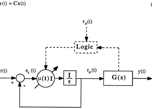
A control structure that ensures that the control u(t) will never saturate is shown in figure 3.3. The time-varying rate, introduced in this section, will be used as a Reference Governor (RG).

r(t) r(t + e(t) u(t) u(t) y(t)

_RG~

K(s)

sat

G(s)

Compensator Saturation Plant

Figure 3.3: Control structure with the RG operator

4. Description of the Control Structure with the Operator RG

In the proposed control structure shown in figure 3.3 the Reference Governor will mask out "large" references so they will not enter into the closed loop system. Choosing the Reference governor appropriately one can ensure that the controls never saturate so that the feedback system operates linearly.

To facilitate our discussion let us assume the following models for the systems shown in figure 3.3.

Page 9

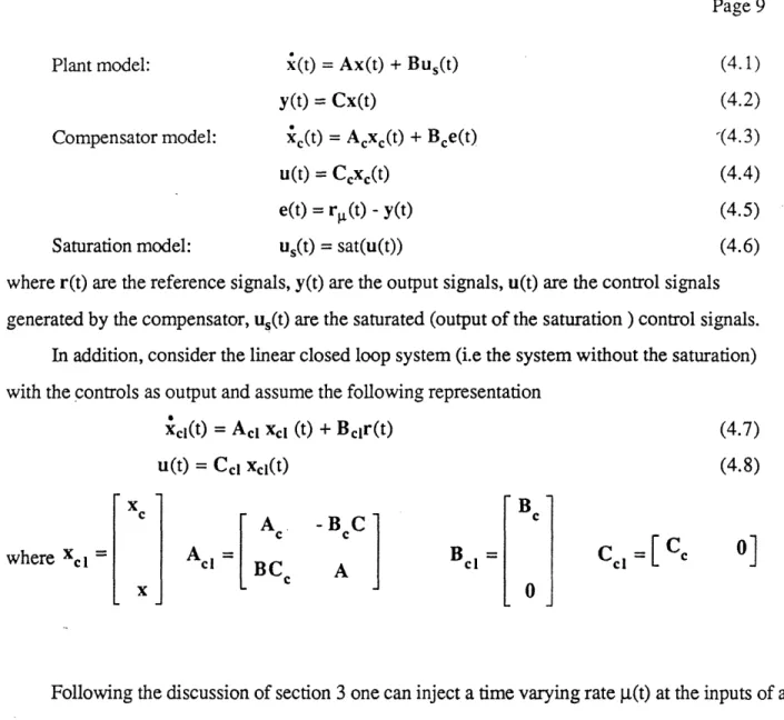
Plant model: x(t) = Ax(t) + Bus(t) (4.1)

y(t) = Cx(t) (4.2)

Compensator model: xc(t) = Acxc(t) + Bce(t) '(4.3)

u(t) = Ccxc(t) (4.4)

e(t) = r,(t) - y(t) (4.5)

Saturation model: U,(t) = sat(u(t)) (4.6)

where r(t) are the reference signals, y(t) are the output signals, u(t) are the control signals generated by the compensator, u,(t) are the saturated (output of the saturation ) control signals.

In addition, consider the linear closed loop system (i.e the system without the saturation) with the controls as output and assume the following representation

xCI(t) = Acl xcl (t) + Bclr(t) (4.7)

u(t) = Ccl xcl(t) (4.8)

where X = Al = _{BC B cc C ]}

Following the discussion of section 3 one can inject a time varying rate g(t) at the inputs of a

linear time invariant system and the outputs of that system will remain bounded. Consider the closed loop system (4.7)-(4.8) and assume that a time-varying rate (4.9)-(4.11) is introduced at the references as shown in figure 4.1

r(t) %(t),,t uOt)

L .

I

K(

Figure 4.1: The basic system for calculating g(t).

Page 10

er (t = r(t) - rg(t) (4.10)

rg(t) = z(t) (4.11)

As in section 3, the time varying gain It(t) will be chosen so that if r(t) is small enough never to cause control saturation then r(t) = rj,(t), in contrast, if r(t) is large, then ti(t) will limit the references so that the controls will remain bounded. We now combine the dynamics of the rate limiter (4.9)-(4. 11) with the dynamics of the closed loop system (4.7)-(4.8) to obtain an augmented system

ia(t) = Aaxa(t)+Bai(t)er(t) (4.12)

u(t) = CaXa(t) (4.13)

XclzZt>(t) 0 0

where X (t) = _{L I (t)} C a =B _{a Bcl Al a} [ C=0 _a CC] The objective here is to construct It(t), 0 < jl(t) < o, in such a way so that for any error er(t) the controls u(t) never saturates. This is similar to designing a time-varying rate so that the output of a linear system remains bounded (section 3). At first, a function g(x) and a set BA,C have to be defined. The symbols g(x) and BA,C should be thought as generic symbols and, when they are used, they are always defined to avoid confusion.

g(xaO): g(xaO) = Wlu(t)lo (4.14)

where xa(t) = Aaxa(t); xa(O) = XaO (4.15)

u(t) = CaXa(t) (4.16)

BA,C = { X: g(x) < 1 } (4.17)

For the function g(x) to be finite the linear system in eq. (4.15) has to be neutrally stable. Even if the plant is unstable the compensator has been designed to stabilize it and the system (4.15) is always neutrally stable. Consequently, the construction of Sg(t) is given by:

Construction of gt):

For every time t choose g(t) as follows

a) if Xa(t)E IntBA,C then Lt(t) = oo which implies that r(t) = r,(t) (4.18) b) if xa(t)E BdBA,C then choose the largest 1t(t) such that (4.19)

Page 11

g(xa (t)+£ [ A a xa (t)+Bat)e (t)er(t)]) - g(xa(t))

lim sup •< 0

£~~E0~~~~~O~~ £E~ ~(4.20)

or for the points where g(x) is differentiable choose It(t) such that

0 < p(t) < oo (4.21)

Dg(xa(t))[Aaxa(t)+Bag(t)er (t)] < 0 V t > 0 (4.22) where Dg(xa(t)) is the Jacobian matrix of g(xa(t)) as in definition 3.2.

c) if Xa(t)O BA,C then choose g(t), 0 < AL(t) < o such that the expression (4.20) is

minimum.

The closed loop system with the RG operator has the following good properties.

a) The controls in the closed loop system will never exceed the limits of the saturation and thus the direction of the control vector is not affected by the saturation. Hence, any inversion of the plant by the compensator is not prevented.

b) Integrators or slow dynamics in the compensator do not windup. The main disadvantage of this method is that the construction of g(t) requires the

measurement of the plant states. More research is needed to assess if estimates of the states can be

used to approximate the real gt(t).

It is clear that in principle this control structure can be used for any plant and any compensator as long as the linear closed loop system is stable (true for all sensible control

systems). Because of the difficulty to compute gL(t), it is recommended to use the control structure with the operator RG in feedback system with unstable plants and/or unstable compensator only. For control systems with stable open loop plants and stable compensators one can use the

Page 12

rg(t)

r --- ILogic -

-r(t) e, r e ( ' u(t) us(t,(t) ) y(t)

t

K (s)

sat

G(s)

Figure 4.2: Control structure with the operator RG.

4.1 Stability Analysis for the Control Structure With the RG

The simple closed loop system form r(t) to r,(t) (which is part of figure 4.2) is given by the

following:

i(t) = L(t)(r(t) - z(t)) (4.23)

rpt(t) = z(t) (4.24)

The system (4.23)-(4.24) is a BIBO stable system, i.e. for bounded r(t) the signal r,(t) is also bounded. This can be shown formally by using Lyapunov stability theory with a Lyapunov function of V = zT(t)z(t) where V = 2,t(t)zT(t)(r(t) - z(t)). If r(t) is bounded the function 'V is

negative definite for large z(t) and thus, z(t) will be bounded.

With the RG operator the controls never saturate so the system from r,(t) to y(t) (which is part of figure 4.2) is a linear system; it is also assumed to be stable since one of the purposes of K(s) is to stabilize the linear feedback system. As a result, the control system from r(t) to y(t) is BIBO stable. This is an important fact because when the open loop plant is unstable the linear control system in the present of saturation may not be BIBO stable for all reference signals.

Since the RG operator is outside of the closed loop system, when disturbances are present one cannot guarantee that the control will not saturate. In fact, there always exists a disturbance that will cause saturation and instability. The following analysis is done only for output disturbances

Page 13

d(t), similar analysis can be performed for other type of disturbances as well.

It is clear that if r(t) is chosen so that the controls will reach the saturation limits, then there is a disturbance with Ild(t)lIo < c, Ve > 0 such that the controls will exceed the limits of the

saturation. To avoid that, one can introduce an artificial saturation level s = [ sl sm]Twith si< 1 and choose it(t) so that the references will never cause the controls of the system to exceed the artificial saturation limit s. Then Loo, bounds can be defined, as we shall do in theorem 4.1, for the disturbances so that if the disturbances do not violate those Lo bounds the controls will always remain within the real saturation limits.

In effect, the controls action can be used, partly, to track commands (llui(t)ll, < si) and, partly, to reject disturbances (llui(t)lloo l-si). -The artificial saturation s is "reserving" part of the control action for command following and the rest of the control action is used for disturbance rejection. In theorem 4.1 the relationship (trade-offs) between s and the Lo, bound on the disturbances that can be rejected will be given.

To ensure that only part of the control is used for command following the operator RG can be used to guarantee that Ilui(t)llo, < si. The computation of Cg(t) for this case is similar to the case where the saturation limit is 1. For example, in the computation of ,g(t) one could scale the compensator so that the control saturation limits instead of s they would be 1. In the implementation, by rescaling the compensator, the actual saturation levels will be s again.

Theorem 4.1 r[121: If the RG operator is used in any feedback system so that the controls (llu i(t)llo < si ), for some vector s the following is true. With zero initial conditions, the closed loop system with the RG operator will have bounded controls (Ilu(t),o < 1) and bounded outputs for any reference and for output disturbances that satisfy the following condition.

s 1, 1.... Ilhm

11

ll

1

s .. . . .

... + <" (4.25)

sm Mhm 1 Ill .... Mm m Ill m Ildm I1ooJ 1

where hij is impulse response of the ijth element of the following transfer function matrix

H(s) = [I + K(s)G(s)]-lK(s) (4.26)

From the previous discussion theorem 4.1 can be used to illustrate the trade-offs between "good" command following and "good" disturbance rejection. There are two ways to use theorem

Page 14

4.1.

(a) If we know upper bounds on the output disturbances that exist in the operating

environment of the control system, the following is true; one can compute the artificial saturation s so that all possible disturbances will be rejected. These upper bounds usually come from

experimental data and the specific operating environment of the system. Then the vector s is computed by the following:

S1ll

<

Ilhl

1

... <- ... .. + ' (4.27)

s

llh

An operator RG will be included in the control system to guarantee that the references will never cause the controls to exceed the artificial saturation s. In this context, if si, for some i, is negative then there exists a disturbance that will cause the system to saturate even if r(t) = 0 for all t. If si is positive, for all i, then there is a disturbance (dj(t) = Ildj(t)lloosign(hij), for some i) with magnitude within the specified upper bounds and some reference, to cause the controls to reach the limits of the real saturation (±1). In that sense theorem 4.1 is not conservative.

(b) If the disturbances are not known then the control designer has to define the artificial saturation s. The value of s should be specified so that with, Ilu(t)lloo, < s, there is "enough" control action for the system to perform (command following) well. One can compute s by using

experimental data, the specifications of the control system, and the specific application. With the value of s one can compute an upper bound for the disturbances that will never cause saturation (+1) as follows: lhl1 1 .... Ilhll [dl lloo 1 Sl

l...

_m

From theorem 4.1 (expression 4.25) is evident that the smaller the disturbances (in the operating environment of the system) the better the command following.

In addition to disturbances, modelling errors can cause the feedback system to saturate and thus degrade the performance or even to drive the system unstable. At this point, it is not clear how

Page 15

to define a class of modelling errors so that the closed loop system with the RG operator will remain stable in the presence of those modelling errors.

5.2 Simulation of the F16 Aircraft

As it was described previously the introduction of the saturation in the a closed loop system when the open loop plant is unstable can

(a) cause instability of the closed loop system (b) cause integrator windups

(c) alter the directions of the controls and thus affect the performance of the system. The purpose of the next example is to illustrate these problems and to show how the new control design method solves these problems.

Consider a model of the AFTI- 16 (Advanced Fighter Technology Integration) aircraft, which is a modified F- 16 aircraft. The following linear time invariant model is an approximation of the aircraft longitudinal dynamics at 3,000 ft altitude and .6 Mach velocity [12].

-. 0151 -60.5651 0 -32.174 -2.516 -13.136 -. 0001 -1.3411 .9929 0 -. 1689 -.2514 ~t) = .00018(t)~~(t + .00018 43.2541 -.86939 0 - 17.251 -1.5766 u s 0 0 1 0 0 0 (4.29) y(t) 0 0 0 1 x(t) (4.30) and in compact form

x(t) = Ax(t) + Bus(t) (4.31)

Page 16

u(t) forward velocity (ft/sec)

c(t) angle of attack (deg) where x(t)=

q(t) pitch rate (deg/sec)

0(t) pitch angle (deg)

(4.33)

F

6(t) elevator angle (deg) limitat250

u(t) )=

[ f(t) flaperon angle (deg) limit at 250

(4.34)

ac(t) angle of attack (deg) y(t) =

0(t) pitch angle (deg)

- (4.35)

Assume that we wish to design a closed loop system so that the F16 follows angle of attack and pitch attitude with zero steady state error required for step commands. Linear control theory will be used to design the closed loop system, then the linear design will be modified as indicated previously with a time varying rate gt(t). Finally, simulations will be performed to assess the benefits of the new design methodology.

To obtain the linear closed loop system, integrators have to be added at the controls; and the augmented system is given by the following

x a (t) = AaXa(t) + BaUa(t) (4.36) (4.36) y(t) = CaXa(t) (4.37) u(t) =-uSW U W a(t) (4.38)(4.38) where A [B A

]

°]

c=[

]

A linear compensator was designed for the augmented system to control the angle of attack and the pitch angle tracking errors. The LQG/LTR methodology was used to design the

Page 17

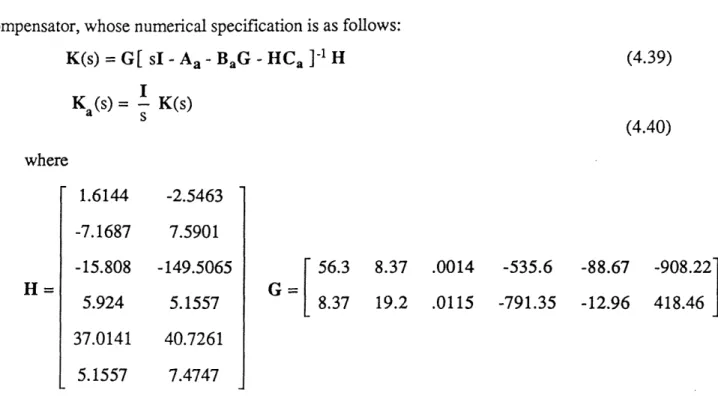
compensator, whose numerical specification is as follows:

K(s) = G[ sI - Aa - BaG - HCa ]-1 H (4.39) Ka(s) = K(s) (4.40) where 1.6144 -2.5463 -7.1687 7.5901 -15.808 -149.5065 56.3 8.37 .0014 -535.6 -88.67 -908.22 5.924 5.1557 G 8.37 19.2 .0115 -791.35 -12.96 418.46 37.0141 40.7261 5.1557 7.4747

It is assumed that the G(s)K(s) loop is the desired forward loop transfer matrix. If it is not, then the linear compensator has to be redesigned. Figure 4.3 shows the control feedback system with the RG operator.

r(t) RG r(t) e(t) u U(t) u(t)5 F16 Y (t)Y

Figure 4.3: Closed loop system for the F16 example with RG. We now deal with a multivariable control system for an unstable open loop plant with integrators and a saturation element in the forward loop. Without the RG operator the control system is expected to have the following problems (a) for certain references r(t) the outputs y(t) will be unbounded, (b) integrator windups may be present, and (c) the saturation can alter the direction of the controls and thus degrade the transient performance of the system.

Three types of simulation were performed for the closed loop system shown in figure 4.3. These different types of simulation are the following:

1) The first simulation is for the linear system. Again we assume that the compensator K(s) we designed yields desirable linear responses.

Page 18

2) In the second simulation the saturation element is added to the linear system, us(t) = sat(u(t)), without any other modifications. This simulation is referred to as the simulation for the

system with saturation.

3) In the third simulation us(t) = sat(u(t)), and g(t) is computed entirely on-line by the method given in section 5.2.2. The simulation was performed in a Macintosh 512K and it required approximately 15-16 hours. This simulation is referred to as the simulation of the system with

saturation and the RG.

At first, the linear system was simulated for r [0 10]Tcorresponding to a 100 pitch angle with zero (trim) angle of attack. Figures 4.4 and 4.5 show the output and control responses of the linear system. Note that the controls have "impulsive" action at the beginning and they exceed by far the 250 limits so saturation is expected. Also note that the maximum flaperon control value is

approximately 83°.

We remark that the quality of the linear output transients (figure 4.4) are not particularly "nice" due to the overshoots present. However, for the sake of comparisons that follow we shall assume that they represent desirable shapes.

Figures 4.6 and 4.7 show the output and control responses of the system with saturation. The closed loop system for the reference input r = [ 0 10]Tis unstable. Note that, in general, when the open loop system is unstable and saturation at the controls is present the resulting control system is only locally stable.

Figures 4.8 and 4.9 show the output and control responses of the system with saturation and the RG operator. The stability of the closed loop control system is recovered and the shape of the transient response is similar ( but slower, as expected) to the linear response. Compare figures 4.4 and 4.8; they are almost identical !!!. Also, the controls u(t) never exceed the saturation limits, as guaranteed by the design methodology.

Figure 4.10 show the modified reference rm2(t). Since the first reference is zero the rml (t) is zero Vt and it was not plotted. Note that the rm2(t), commanded pitch attitude, starts at =3° and ramps up to the desired steady state value of 100. The reason that the rm2(t) is initially =30 is

because the linear system with an rm2(t) of =3° will have controls with maximum at =25° (remember that with an rm2(t) of =100 the controls had a maximum value of =830). Then as the outputs follow the modified references the rg.(t) approaches r(t) in such a way that the controls will never exceed the saturation limits.

Page 19

Output y(t) for the F 16 closed loop system wvith r=[ 0 10 ]

18.00

14.00

10.00

-

6.00

0.00

2.00

4.00

6.00

8.00

10.00

Figure 4.4: Output response of the F16 linear system, (r = [0 10]T).

Control in the F 16 closed loop system vith r=[ 0 10

]

T

90.0

60.0

30.0

o 0.0

-30.0

-60.0

0.0

2.0

4.0

6.0

8.0

10.0

Page 20

Output in the F16 closed loop system with r=[ 0 10 ] T

100000.0

80000.0

Figure 4.6: Output response of the F16 system with saturation, (r = [O 10]T).

Control in the F 16 closed loop systemvith r=[ 0

]

300000.0 180000.0

2.

-60000.0

o

Time (sec.)

Page 21

Output for the F16 closed loop system with r=[ 0

]T

18.00

14.00

Figure 4.8: Output response for the F16 system with saturation and the RG, (r = [0 10]T).

Control for the F 16 closed loop system vith r=[ 0

]

90.0

60.0

W 30.0

Page 22 12.0 r2 (t_) 9.6 12.0 7.2 8.0 r~(t)2 4.8 4.0 2.4 0.0 0.0 0.2 0.4 0.6 0.0 0.0 2.0 4.0 6.0 8.0 10.0 Time(sec.)

Figure 4.10: r~2(t), the commanded pitch, in the F16 system with saturation and the

RG, (r = [0 10]T). Insert: Blowup with 0 < t < .6.

A second simulation was performed for the same system with reference r = [2.5 2.5]T. Now we are commanding simultaneously 2.50 angle of attack and pitch. Figures 4.11 and 4.12 show the output and control responses of the linear system. Again the controls exceed the limits of 25° and saturation is expected.

Figures 4.13 and 4.14 show the response of the system with saturation from the output response one can see that the integrators windup although, now, the closed loop system is stable. In addition, the direction of the outputs is not similar to the direction of the outputs in the linear system and thus the control system does not behave as it was designed to behave.

Figures 4.15 and 4.16 show the output and control response of the system with saturation and the RG. The controls never exceed the limits of the saturation and thus integrator windups are not present. The output response verify the absence of integrator windups. The output response is slower because of the limited controls but the direction of the outputs is similar to that of the linear system. Figure 4.17 show the modified reference rg(t).

Page 23

Output for the F16 closed loop system with r=[ .25 .25

7.5 6.0 4.5

3.0

1.5

0.0

0.0

2.0

4.0

6.0

8.0

10.0

Figure 4.11: Output response for the F16 linear system, (r = [2.5 2.5]T).

Control for the F16 closed loop system with r=[ 2.5 2.5 ]T

8.0

-16.0

-28.0

-40.0

0.0

2.0

4.0

6.0

8.0

10.0

Page 24

Output for the F16 closed loop system ith r=[ .25 .25 ]T

7.5

6.0

3.0

1.5

Figure 4.13: Output response for the F16 system with saturation, (r = [2.5 2.5]T).

Control for the F16 closed loop system vith r=[ 2.5 2.5] T

20.0

8.0

-4.0

-16.0

-28.0

-40.0

0.0

2.0

4.0

6.0

8.0

10.0

Page 25

Output for the F 16 closed loop system with r=[

2.5]

6.25

3.75

'; 2.50

o 1.25

Figure 4.15: Output response for the F16 system with saturation and the RG, (r = [2.5 2.5]T).

Control for the F 16 closed loop system vith r=[ 2.5 2.5 ]T

20.0

-4.0

-16.0

Page 26 3.0 2.4 rl (1) = ra(t ) 1.8 r (t) 1.2 0.6 0.0 0.0 2.0 4.0 6.0 8.0 10.0 Time (sec.)

Figure 4.17: r,(t) in the F16 system with saturation and the RG, (r = [2.5 2.5]T).

5. Concluding Remarks

In this paper it has been shown how that the operator RG can be used to design control systems for plants with multiple saturations. The operator RG preprocesses the reference signals in such a way so that the references never cause the controls in the closed loop system to saturate. Typically, sudden large step commands are translated by the RG operator into slower commands, so as to allow the limited controls not only to stabilize the system but also to eventually track the reference. Thus the signals in the closed loop system remain bounded for any reference and if integrators are present in the loop they never windup. The control structure with the operator RG can be used in any closed loop stable linear feedback system.

In addition, we have shown how to define disturbance sets so that, if the disturbances belong to these sets, then the outputs of the system remain bounded. With this new design methodology one can distribute the control action among rejecting disturbances and following references as it is needed for specific applications.

The main benefits of the methodology are that it leads to controllers with the following properties:

Page 27

(a) The signals that the modified references never cause saturation.

(b) Possible integrators or slow dynamics in the compensator never windup. (c) The closed loop system has inherent stability properties.

These properties were demonstrated in simulations of the F8 aircraft (stable) model and an academic example.

6. References

[1] M. Athans, P.L. Falb, Optimal Control, New York, McGraw-Hill, 1966.

[2] C.A. Harvey, " On Feedback Systems Possessing Integrity With Respect to Actuators Outages", Proceedings of the ONR/MIT Workshop on Resent Developments in the Robustness Theory of Multivariable Systems, LIDS-R-954, M.I.T., Cambridge, MA, April 25-27, 1979.

[3] P. Molander and J.C. Willems, " Robustness Results For State Feedback Regulators", Proceedings of the ONR/MIT Workshop on Resent Developments in the Robustness Theory of Multivariable Systems, LIDS-R-954, M.I.T., Cambridge, MA, April 25-27, 1979.

[4] A. Weinreb and A.E. Bryson," Optimal Control of Systems with Hard Control Bounds" IEEE Transactions on Automatic Control, Vol. AC-30, No. 11, November 1985, pp. 1135-1138.

[5] P. Gutman and P. Hagander, " A New Design of Constrained Controllers for Linear Systems", IEEE Transactions on Automatic Control, Vol. AC-30, No. 1, January 1985, pp. 22-33.

[6] A. H. Glattfelder and W. Scaufelberger," Stability Analysis Of Single Loop Control Systems with Saturation and Antireset-Windup Circuits", IEEE Transactions on Automatic Control, Vol. AC-28, No. 12, December 1983, pp. 1074-1081.

[7] N. Rouche, P. Habets and M Laloy, Stability Theory by Lyapunov's Direct Method, New York, Springer-Verlag, 1977.

[8] P. Kapasouris and M. Athans, " Multivariable Control Systems with Saturating Actuators Antireset Windup Strategies", Proceedings of the American Control Conference, Boston, MA,

1985, pp. 1579-1584.

[9] J.C. Doyle, R.S. Smith and D.F. Enns, " Control of Plants with Input Saturation Nonlinearities", Proceedings of the American Control Conference. Minneapolis, MN, 1987, pp.

Page 28 1034-1039.

[10] P. Kapasouris, Design for Performance Enhancement in Feedback Control Systems with

Multiple Saturating Nonlinearities, Ph.D. Thesis, Department of Electrical Engineering, M.I.T.,

Boston, MA, February 1988.

[11] P. Kapasouris, M. Athans and G. Stein, "Design of Feedback Control Systems for Stable Plants with Saturating Actuators",to appear in the Proceedings of the Conference on Decision and Control, Austin, TX, 1988.

[12] D. Brett Ridgely, "Use of Entire Eigenstructure Assignment with High-Gain Error-Actuated Flight Control Systems", S.M. Thesis, AFIT/GAE/AA81D-24, Air Force Institute of Technology, Wright-Patterson Air Force Base, Ohio, December 1981.