HAL Id: tel-01312183
https://tel.archives-ouvertes.fr/tel-01312183
Submitted on 4 May 2016HAL is a multi-disciplinary open access
archive for the deposit and dissemination of sci-entific research documents, whether they are pub-lished or not. The documents may come from teaching and research institutions in France or
L’archive ouverte pluridisciplinaire HAL, est destinée au dépôt et à la diffusion de documents scientifiques de niveau recherche, publiés ou non, émanant des établissements d’enseignement et de recherche français ou étrangers, des laboratoires
Automatic target classification based on radar
backscattered ultra wide band signals
Mahmoud Khodjet-Kesba
To cite this version:
Mahmoud Khodjet-Kesba. Automatic target classification based on radar backscattered ultra wide band signals. Other. Université Blaise Pascal - Clermont-Ferrand II, 2014. English. �NNT : 2014CLF22506�. �tel-01312183�
N° d’ordre D. U : 2506 E D S P I C : 671
U
NIVERSITE
B
LAISE
P
ASCAL
-
C
LERMONT
II
E
COLE
D
OCTORALE
S
CIENCES
P
OUR L
’I
NGENIEUR DE
C
LERMONT
-F
ERRAND
T h è s e
Présentée par
Mahmoud Khodjet
Mahmoud Khodjet
Mahmoud Khodjet
Mahmoud Khodjet----Kesba
Kesba
Kesba
Kesba
pour obtenir le grade de
DDDD
O C T E U R D
O C T E U R D
O C T E U R D
O C T E U R D
’’’’
UUUU
N I V E R S
N I V E R S
N I V E R S
N I V E R S I T É
I T É
I T É
I T É
SPECIALITE :
E
LECTROMAGNÉTISMEAUTOMATIC TARGET CLASSIFICATION BASED ON RADAR
BACKSCATTERED ULTRA WIDEBAND SIGNALS
Soutenue publiquement le 06 Novembre 2014 devant le jury :
Mme Hélène Roussel Président
M. Christian Brousseau Rapporteur
M. Dong Ryeol Shin Examinateur
M. Andrea Bianchi Examinateur
M. Christophe Pasquier Examinateur
Mme Claire Faure Examinateur
M. Khalil El Khamlichi Drissi Directeur de thèse
Blaise Pascal University
Doctoral School of Engineering Science
Sungkyunkwan University
Department of Electrical and Computer Engineering
College of Information and Communication Engineering
Doctoral Thesis
Speciality: Electromagnetism
Automatic Target Classification based on Radar
Backscattered Ultra WideBand Signals
by
Mahmoud Khodjet-Kesba
Pr Khalil El Khamlichi Drissi, Supervisor Pr Sukhan Lee, Supervisor
Pr H´el`ene Roussel, Rapporteur Pr Christian Brousseau, Rapporteur
Pr Dong Ryeol Shin, Member Pr Andrea Bianchi, Member Dr Christophe Pasquier, Member
Dr Claire Faure, Member November 06, 2014
Acknowledgements
The accomplishment of this thesis was made possible with the help and support of many people. First of all, I would like to thank my two advisors. Pr Khalil El Khamlichi Drissi of Blaise Pascal University, he always believed on me, helped and encouraged me through some rough periods. I admire his devotion and efficiency. Pr Sukhan Lee of Sungkyunkwan University, I thank him for his guidance, motivation and technical assistance with my research. He welcomed me and helped me to adapt in Korea, this beautiful country that I discovered and which has a special place in my heart.
I am also grateful to Claire Faure, Kamal Kerroum and Christophe pasquier for the advices, comments and stimulating discussion I received from them.
I am grateful to the rapporteurs of my defense committee: Professor H´el`ene Roussel of the Pierre and Marie Curie University (Paris 6) and Professor Chris-tian Brousseau of the Rennes 1 University. I am also grateful to Professor Dong Ryeol Shin of the Sungkyunkwan University and Professor Andrea Bianchi of the Sungkyunkwan University for their highly appreciated participation in the defense committee.
I owe the utmost gratitude to my parents for their love and for their endless support in whatever I wanted to do. It is to them I dedicate this thesis.
Abstract
The objective of this thesis is the Automatic Target Classification (ATC) based on radar backscattered Ultra WideBand (UWB) signals. The classification of the tar-gets is realized by making comparison between the deduced target properties and the different target features which are already recorded in a database. First, the study of scattering theory allows us to understand the physical meaning of the extracted features and describe them mathematically. Second, feature extraction methods are applied in order to extract signatures of the targets. A good choice of features is important to distinguish different targets. Different methods of feature extraction are compared including wavelet transform and high resolution techniques such as: Prony’s method, Root-Multiple SIgnal Classification (Root-MUSIC), Estimation of Signal Parameters via Rotational Invariance Techniques (ESPRIT) and Matrix Pencil Method (MPM). Third, an efficient method of supervised classification is necessary to classify unknown targets by using the extracted features. Different methods of clas-sification are compared: Mahalanobis Distance Classifier (MDC), Na¨ıve Bayes (NB),
k-Nearest Neighbors (k-NN) and Support Vector Machine (SVM). A useful classifier
design technique should have a high rate of accuracy in the presence of noisy data coming from different aspect angles. The different algorithms are demonstrated using simulated backscattered data from canonical objects and complex target geometries modeled by perfectly conducting thin wires. A method of ATC based on the use of Matrix Pencil Method in Frequency Domain (MPMFD) for feature extraction and MDC for classification is proposed. Simulation results illustrate that features ex-tracted with MPMFD present a plausible solution to automatic target classification. In addition, we prove that the proposed method has better ability to tolerate noise effects in radar target classification. Finally, the different algorithms are validated on experimental data and real targets.
Keywords: Backscattering, Ultra wideband radar, Feature extraction,
R´
esum´
e
L’objectif de cette th`ese est la classification automatique des cibles (ATC) en utilisant les signaux r´etrodiffus´es par un radar ultra large bande (UWB). La classifi-cation des cibles est r´ealis´ee en comparant les signatures des cibles et les signatures stock´ees dans une base de donn´ees. Premi`erement, une ´etude sur la th´eorie de dif-fusion nous a permis de comprendre le sens physique des param`etres extraits et de les ´exprimer math´ematiquement. Deuxi`emement, des m´ethodes d’extraction de param`etres sont appliqu´ees afin de d´eterminer les signatures des cibles. Un bon choix des param`etres est important afin de distinguer les diff´erentes cibles. Diff´erentes m´ethodes d’extraction de param`etres sont compar´ees notamment : m´ethode de Prony, Racine-classification des signaux multiples (Root-MUSIC), l’estimation des param`etres des signaux par des techniques d’invariances rotationnels (ESPRIT), et la m´ethode Matrix Pencil (MPM). Troisi`emement, une m´ethode efficace de classifi-cation supervis´ee est n´ecessaire afin de classer les cibles inconnues par l’utilisation de leurs signatures extraites. Diff´erentes m´ethodes de classification sont compar´ees no-tamment : Classification par la distance de Mahalanobis (MDC), Na¨ıve Bayes (NB),
k-plus proches voisins (k-NN), Machines `a Vecteurs de Support (SVM). Une bonne technique de classification doit avoir une bonne pr´ecision en pr´esence de signaux bruit´es et quelques soit l’angle d’´emission. Les diff´erents algorithmes ont ´et´e valid´es en utilisant les simulations des donn´ees r´etrodiffus´ees par des objets canoniques et des cibles de g´eom´etries complexes mod´elis´ees par des fils minces et parfaitement con-ducteurs. Une m´ethode de classification automatique de cibles bas´ee sur l’utilisation de la m´ethode Matrix Pencil dans le domaine fr´equentiel (MPMFD) pour l’extraction des param`etres et la classification par la distance de Mahalanobis est propos´ee. Les r´esultats de simulation montrent que les param`etres extraits par MPMFD pr´esentent une solution plausible pour la classification automatique des cibles. En outre, nous avons prouv´e que la m´ethode propos´ee a une bonne tol´erance aux bruits lors de la classification des cibles. Enfin, les diff´erents algorithmes sont valid´es sur des donn´ees exp´erimentales et cibles r´eelles.
Mots cl´es: R´etrodiffusion, Radar ultra large bande, Extraction de param`etres, Classification automatique de cibles, La m´ethode Matrix Pencil.
Contents
List of Figures x
List of Tables xiii
List of Abbreviations xiv
1 Introduction 1
1.1 Overview . . . 1
1.2 Contributions and thesis organization . . . 4
1.3 List of publications . . . 5
2 Electromagnetism and Scattering theory 8 2.1 Introduction . . . 8
2.2 Notions of electromagnetism . . . 8
2.2.1 Maxwell’s equations . . . 8
2.2.2 Time harmonic fields . . . 9
2.2.3 Propagation equations in unbounded media . . . 10
2.3 Scattering theory . . . 10
2.3.1 The radar cross section . . . 11
2.3.2 Frequency regions . . . 12
2.3.3 Propagation mechanisms . . . 13
2.3.4 Singularity Expansion Method . . . 15
2.3.6 Reduced complexity model . . . 17
2.4 Field regions . . . 19
2.4.1 Reactive near field region . . . 19
2.4.2 Radiating near field (Fresnel) region . . . 19
2.4.3 Far field (Fraunhofer) region . . . 20
2.5 Theoretical analysis of the backscattered field from canonical objects 20 2.5.1 The conducting sphere . . . 20
2.5.2 The thin wire . . . 27
2.6 Conclusion . . . 32
3 UWB Radar 33 3.1 Introduction . . . 33
3.2 Radars . . . 33
3.2.1 Information available from a radar . . . 34
3.2.2 The deficiencies of conventional radars . . . 37
3.3 Historical review of UWB radar . . . 38
3.4 Definition of UWB . . . 40
3.5 Application of ultra-wideband sensing . . . 43
3.6 Advantages of Ultra-Wideband Radar . . . 46
3.7 UWB techniques . . . 47
3.7.1 Impulse radar . . . 47
3.7.2 Noise radar . . . 50
3.7.3 Step frequency radar . . . 51
3.7.4 Frequency modulated continuous wave radar . . . 53
3.7.5 Conclusion . . . 54
3.9 Conclusion . . . 57
4 Radar automatic target classification 59 4.1 Introduction . . . 59
4.2 Feature extraction . . . 59
4.2.1 Wavelet transform . . . 60
4.2.2 High resolution methods . . . 64
4.3 Classification methods . . . 78
4.3.1 Introduction . . . 78
4.3.2 Cross Validation . . . 78
4.3.3 The Mahalanobis Distance Classifier . . . 79
4.3.4 Na¨ıve Bayes . . . 80
4.3.5 k-NN . . . . 81
4.3.6 Support Vector Machine . . . 82
4.4 Conclusion . . . 88
5 Simulation and experimental results 89 5.1 Introduction . . . 89
5.2 Simulation results of backscattered fields from canonical objects . . . 89
5.2.1 Presentation of FEKO and the simulation parameters . . . 90
5.2.2 The signals in time domain . . . 90
5.2.3 The signals in Frequency domain . . . 92
5.3 Feature extraction results . . . 92
5.3.1 Comparison between analytical and measured CNRs . . . 92
5.3.2 Matrix Pencil Method in Time Domain . . . 98
5.3.3 Matrix Pencil Method in Frequency Domain . . . 102
5.5 Classification of complex objects in white Gaussian noise . . . 108
5.5.1 Classifier Design . . . 109
5.5.2 Simulation results . . . 111
5.6 Experimental results . . . 116
5.6.1 Measurement setup . . . 116
5.6.2 Data processing and feature extractions . . . 118
5.6.3 Classification results . . . 121
5.7 Conclusion . . . 125
6 Conclusions 127
A Analytical expression of the sphere’s residues 131
List of Figures
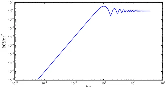
2.1 The RCS of a sphere as function of k a (k is the wave number and a
is the radius of the sphere) . . . 13
2.2 Three field regions surrounding a scattering object . . . 19
2.3 Normal plane wave incidence (θ = 90◦) on a conducting sphere . . . . 21
2.4 Magnitude of the backscattered field from a sphere (k is the wave number and a is the radius of the sphere) . . . . 23
2.5 Addition of specular and creeping waves . . . 23
2.6 Complex Natural Resonances of a conducting sphere . . . 26
2.7 Geometry of the thin wire . . . 27
2.8 Plot of the backscattered field of a thin wire for θi = θ0 = 90◦ . . . . 29
2.9 Overlay plots of the normalized resonant frequencies as computed by the methods of Giri, et al., Tesche and Myers, et al., for the wire with a/L = 0.005 . . . . 31
3.1 The radar system diagram . . . 34
3.2 Schematic of the calculation of the velocity . . . 35
3.3 An air-surveillance radar . . . 36
3.4 Target localization using three radars . . . 36
3.5 A UWB signal is defined to have an absolute bandwidth B≥ 500MHz, or a fractional bandwidth greater than 0.2 . . . 42
3.6 Comparison of various radio system spectrums . . . 42
3.7 The different UWB techniques . . . 48
3.9 Block diagram of a noise radar . . . 50
3.10 Step-frequency waveform . . . 52
3.11 Block diagram of step-frequency radar . . . 53
3.12 The principle of operation of an FMCW radar . . . 54
3.13 Block diagram of an FMCW radar . . . 54
3.14 Overview of the target recognition process . . . 56
4.1 Wavelet decomposition scheme . . . 63
4.2 Optimal separating hyperplane in a two-dimensional space . . . 83
5.1 Example of the three canonical objects . . . 91
5.2 Gaussian pulse time . . . 91
5.3 The backscattered fields form the three canonical objects in the time domain . . . 93
5.4 The backscattered fields from the three canonical objects in the fre-quency domain . . . 94
5.5 The backscattered fields form thin wire (a/L = 0.005) . . . 96
5.6 Normalized CNRs location in the s-plane with different incident angles 97 5.7 Normalized CNRs location in the s-plane with different values of SNR 98 5.8 Simulated signal compared with reconstructed signal by MPMTD . . 100
5.9 Variation of positive imaginary part of the poles with sliding time . . 101
5.10 Simulated signal compared with reconstructed signal by MPMFD . . 103
5.11 k-NN classification accuracy of wavelets . . . 105
5.12 Classification accuracy of wavelets for MDC, k-NN, NB and SVM . . 107
5.13 The 4 target geometries . . . 111
5.14 Simulated signal compared with reconstructed signal by MPMFD . . 114
5.15 The Mahalanobis distance of the object 1 with an aspect angle of 45◦ from the 4 targets . . . 115
5.16 Comparison between the total classification accuracy when using only
Eθ or both Eθ and Eφ . . . 115
5.17 UWB P400 MRM . . . 116
5.18 Radar system . . . 116
5.19 Transmitted waveform . . . 117
5.20 The indoor environment . . . 118
5.21 Raw signal received by the radar . . . 119
5.22 Signatures of the three targets after removing the environment . . . . 120
5.23 Normalized signatures of the three targets . . . 122
5.24 Measured signal compared with reconstructed signal by MPMFD . . 123
5.25 The first three singular values for one angle . . . 124
List of Tables
2.1 Frequency dependence parameters for canonical scattering geometries 18 5.1 Features extracted by MPMTD from a thin wire (l = 3m), a sphere
(r = 0.3 m), and a cylinder (l= 0.6 m, r= 0.2 m) (poles× 109) . . . . 99
5.2 Features extracted by MPMFD from a thin wire (l = 3m), a sphere (r = 0.3 m), and a cylinder (l= 0.6 m, r= 0.2 m) (poles× 108) . . . . 104
5.3 Classification accuracy of each object (%) . . . 108
5.4 Dimensions of the four targets . . . 112
5.5 Classification accuracy of each object (%) . . . 113
List of Abbreviations
ADC Analog to Digital Converter ATC Automatic Target Classification CNRs Complex natural resonances
coif Coiflet
CWT Continuous Wavelet Transform
DARPA US Defense Advanced Research Projects Agency db Daubechies
DSP Digital Signal Processor DWT Discrete Wavelet Transform
ESPRIT Estimation of Signal Parameters via Rotational Invariance Techniques
FCC Federal Communication Commission
FEKO FEldberechnung bei Krpern mit beliebiger Oberflche (German: Field computations involving bodies of arbitrary shape)
FEM Finite Element Method FFT Fast Fourier Transform
FMCW Frequency Modulated Continuous Wave FPGA Field Programmable Gate Array
GPR Ground Penetrating Radar HDTV High Definition Television
IFFT Inverse Fast Fourier Transform
k-NN k-Nearest Neighbors
LPF Low-Pass Filter LS Least-Squares
MDC Mahalanobis Distance Classifier MLFMM Multilevel Fast Multipole Method
MoM Method of Moments MPM Matrix Pencil Method MRM Monostatic Radar Module
NB Naive Bayes
PANs Personal Area Networks PO Physical Optics
PRI Pulse Repetition Interval RFID Radio Frequency Identification Root-MUSIC Root-MUltiple SIgnal Classification
SEM Singularity Expansion Method SNR Signal-to-Noise Ratio
SVM Support Vector Machine TLS Total Least Squares
UMTS Universal Mobile Telecommunications System USB Universal Serial Bus
UTD Uniform Theory of Defraction UWB Ultra Wideband
1
Introduction
1.1
Overview
The work done in this thesis is in the framework of a co-degree program between Pas-cal Institute in Blaise PasPas-cal University (France) and Intelligent Systems Research Institute in SungKyunKwan University (Republic of Korea) under the project enti-tled Cognitive Personal Transport Service Robot sponsored by the Gyeonggi-province International Collaboration Research Project. The project has the following research objectives to accomplish:
• To develop original technologies, as well as designing and demonstrating a
prototype, for the Cognitive Personal Transport Service Robot capable of autonomous and/or semi-autonomous individual robotic and environmentally friendly call taxi service in towns, campuses, and tourist attractions where the driving environments such as roads, traffic signs, moving traffics, pedestrians, trees, animals, etc have to be recognized.
• To explore enabling technologies for extending the devloped Cognitive Personal
technolo-gies to be developed include: Autonomous navigation, Sociable multi-modal human-vehicle interaction and Platforms for software, hardware and network for a cognitive personal transport robot based ride share system.
Autonomous navigation of vehicles is a complex problem that has attracted the attention of the research community and related companies. Systems capable of per-forming efficient and robust autonomous navigation are of interest in many robotic applications such as automatic industry, personal transportation, assistances to dis-abled or elder people, surveillance, etc. In order to perform navigation, the vehicle needs to interact with the environment, and for this purpose different types of sensors can be used for extracting the meaningful information and then making a decision for safe and unmanned navigation. From all of them, vision systems are the most used because they provide very rich information. However, the visual systems can become vulnerable when weather is severe and visibility is low (fogs, night, etc) or when target is well protected and hidden such as deeply beneath the foliage. In this case, using electromagnetic waves can be a good solution for target identification.
In the last fifteen years, the interest in Ultra Wideband (UWB) systems has grown rapidly. One of several applications of the UWB is radar automatic target classifica-tion in autonomous vehicles. UWB radar uses very short duraclassifica-tion pulses resulting in very wideband in frequency domain. The UWB technique has the advantage to be used for localization, target identification, and communication between vehicles. In this thesis, we propose to use UWB radar in order to automatically classify an unknown target. In Automatic Target Classification (ATC), the two main steps are feature extraction and classification. The identification of the target is realized by making comparison between the deduced target properties and the different target features which are already recorded in a database.
A good choice of features is important to distinguish different targets. The best handling of the feature extraction consists of understanding the physical behavior of a radar system in its environment. Based on this understanding, features must then be mathematically described depending on the given requirements. When the target is illuminated by ultra-wideband signals, the scattered transient response in the time domain is composed from two successive parts [1]. First, an impulsive part, corresponding to the early time response, comes from the direct reflection of the incident wave on the object surface. Next, during the late time, the oscillating part arises from resonance phenomena of the target. In the case where targets are perfect conductors, resonances occur outside the object and correspond to surface creeping waves.
Currently, there exist several techniques based on the analysis of the late time impulse response in order to extract Complex natural resonances (CNRs) such as: the E-pulse approach [2], the Tufts and Kumaresan method [3] , and the high resolution methods like Matrix Pencil Method [4]. The late time part of the signal depends, at least theoretically, on the target geometry and its physical properties. Thus, it is independent of the aspect and polarization of the excitation source [5]. However, the automatic determination of the late time is not an easy task [6]. CNRs can be extracted in the frequency domain by using the Cauchy method. In [7], this method is applied to compute the natural poles of an object in the frequency domain; however, in real time applications, this method is inconvenient.
In this thesis, we propose an approach of feature extraction in frequency domain by using Matrix Pencil Method. The proposed method takes into account not only the magnitude of the signal in frequency domain but also its phase. Therefore, all the physical characteristics of the target are taken into account. The physical and geometrical characteristics of the considered object and the incident waveform impact clearly the signatures of the treated targets and contribute efficiently to the
classification of the objects. The separation between the early time and the late time is not necessary by applying the proposed method. Moreover, we propose a powerful method for UWB radar automatic target classification in white Gaussian noise and different aspect angles between the radar and the target. The proposed method is validated on complex objects by simulations and experiments.
1.2
Contributions and thesis organization
The remainder of this dissertation is organized as follows:
• Chapter 2 presents the different models of scattering. In particular, it presents
Singularity Expansion Method (SEM), Geometric Theory of Diffraction (GTD) and its reduced complexity model. The chapter concludes by giving the theo-retical analysis of the backscattered fields from canonical objects.
• Chapter 3 provides an overview of radars and the deficiencies of conventional
radars. Next, it gives the history, definition, application and advantages of UWB radars. This chapter summarizes temporal and frequency techniques used to obtain a UWB spectrum. Finally, it gives an overview of the UWB radar in ATC.
• Chapter 4 presents the methods used for feature extraction including wavelet
transform and high resolution techniques. Next, it presents the methods used for classification which include Mahalanobis Distance Classifier (MDC), Na¨ıve Bayes (NB), k-Nearest Neighbors (k-NN) and Support Vector Machine (SVM). This chapter explains the cross validation method which is applied in order to evaluate and compare the different methods of classification.
• Chapter 5 gives the simulation and experiment results. The chapter proposes
Gaussian noise and different aspect angles between the radar and the target.
• Chapter 6 provides the conclusion. It summarizes the main achievements of
this thesis and outlines future research directions.
The main contributions can be summarized as follows:
• Comparison of different methods of feature extraction in time domain and in
frequency domain.
• Proposition of a feature extraction method, called Matrix Pencil Method in
Frequency Domain (MPMFD), based on the extraction of parameters in fre-quency domain.
• Comparison of different methods of classification including: MDC, NB, k-NN
and SVM.
• Proposition of a powerful method for UWB radar ATC in white Gaussian noise
and different aspect angles between the radar and the target.
1.3
List of publications
This research work resulted in the following publications:
1. Journal papers:
• M. Khodjet-Kesba, K. El Khamlichi Drissi, S. Lee, K. Kerroum, C. Faure
and C. Pasquier, Comparison of Matrix Pencil Extracted Features in Time Do-main And in Frequency DoDo-main for Radar Target Classification, International
Journal of Antennas and Propagation, vol. 2014, Article ID 930581, 9 pages,
2014.
• M. Khodjet-kesba, K. Chahine, k. El khamlichi drissi, and K. Kerroum,
Comparison of Ultra-wideband Radar Target Classification Methods Based on Complex Natural Resonances, PIERS, March 2012, Kuala Lumpur, Malaysia.
• M. Khodjet-Kesba, K. El Khamlichi Drissi, K. Kerroum, C. Faure and
C. Pasquier, The choice by cross validation technique of features extraction method for UWB radar target classification, PIERS, august 2012, Moscow, Russia.
• M. Khodjet-Kesba, K. El Khamlichi Drissi, S. Lee, K. Kerroum, C. Faure
and C. Pasquier, Robust UWB Radar Target Classification in White Gaussian Noise based on Matrix Pencil Method in Frequency Domain and Mahalanobis Distance, International radar conference, 2014, Lille, France.
• M. Khodjet-Kesba, K. El Khamlichi Drissi, S. Lee, K. Kerroum, C. Faure
and C. Pasquier, Caract´erisation Efficiente d’objets Diffractants Dans Le Do-maine Fr´equentiel, CEM 2014, Clermont Ferrand, France.
• S. Lall´ech`ere, S. Girard, M. Khodjet-Kesba, I. El Baba, A. Catrain, K.
Drissi, P. Bonnet, F. Paladian, Confrontation de mesures num´eriques et exp´erimentales pour la caract´erisation de cibles en environnements libre et confin´e, CEM 2014,
Clermont Ferrand, France.
3. National conferences:
• M. Khodjet-Kesba, K. El Khamlichi Drissi, S. Lee, K. Kerroum, C. Faure
and C. Pasquier, Nouvelles approches d’identification d’obstacles en utilisant un Radar UWB, 15eme Journ´ee Scientifique de l’´ecole doctorale Sciences Pour
2
Electromagnetism and Scattering theory
2.1
Introduction
In this chapter we present some notions in electromagnetism. Next, we present the scattering theory where we show the different models of scattering. In particular, Singularity Expansion Method (SEM) , Geometric Theory of Diffraction (GTD) and its reduced complexity model are presented. Then, we talk about the three field regions surrounding a scattering object. Finally, theoretical analysis of the backscattered fields from canonical objects is presented.
2.2
Notions of electromagnetism
2.2.1 Maxwell’s equations
James Clark Maxwell (1831-1879) published a complete form of equations that govern the behavior of the electromagnetic phenomenon, it involves the behavior of two vector fields: the electric field ⃗E, and the magnetic induction ⃗B.
The basic Maxwell equations in derivative form are given in time domain as:
⃗
rot( ⃗E) =−∂ ⃗B
div( ⃗B) = 0 (2.2) ⃗ rot( ⃗B) = µ( ⃗J + ϵ∂ ⃗E ∂t) (2.3) div( ⃗E) = ρ ϵ (2.4) ⃗
J is the electric current density and ρ is the electric charge density. ϵ is the electric
permittivity, and µ is the magnetic permeability. The electric permittivity is related to its relative permittivity ϵr and the permittivity of the vacuum by the relation:
ϵ = ϵ0ϵr. In the same way, the magnetic permeability is related to its relative
permeability and the permeability of the vacuum by the relation: µ = µ0µr. Further
discussion about the physical significance of each of these equations may be found in [8, 9].
The constitutive relations describe the interaction between the fields and the medium of propagation. For a linear, homogenous and isotropic medium these are of the form:
⃗
D = ϵ ⃗E (2.5)
⃗
B = µ ⃗H (2.6)
2.2.2 Time harmonic fields
We usually use the Maxwell’s equations in their harmonic form, by considering that fields and sources have sinusoidal dependence on time. Then, we can write the electric field as:
⃗
E(⃗r, t) = ⃗E(⃗r)ejωt (2.7) and Maxwell’s equations (2.1) and (2.3) become:
⃗
rot( ⃗E) =−jω ⃗B (2.8)
⃗
2.2.3 Propagation equations in unbounded media
We suppose that all sources are putted in the infinite, so they don’t appear in the equations. In an unbounded, linear, homogenous and isotropic media, the Maxwell’s equations allow to deduce the propagation equations in time domain of the electro-magnetic fields ⃗E and ⃗H:
∆ ⃗E− 1 ν2 ∂2E⃗ ∂t2 = 0 (2.10) ∆ ⃗H− 1 ν2 ∂2H⃗ ∂t2 = 0 (2.11)
where ∆ is the Laplacian. The propagation speed of the wave in infinite media is:
ν = √1
ϵµ (2.12)
We seek solutions of fields that vary in time under the sinusoidal form. The general form of the elementary solution is:
⃗
E0 ej(ωt−⃗k⃗r) (2.13)
⃗
E0 is a constant vector, ⃗k is the wave vector. This solution represents a plane wave
because all points of a wave plan perpendicular to the vector of propagation ⃗k have the same vibratory behavior.
The wave number k is defined as follows:
k = 2π
λ (2.14)
where λ is the wavelength.
2.3
Scattering theory
Scattering is defined as the redirection of radiation out of the original direction of propagation, usually due to interactions of the wave with the target. When the
scattering field is radiated in the backward direction to the incident wave, it is called backscattered field.
Different models have been proposed for scattering using either resonances or scat-tering centers. Baum [10], proposed a mathematical model in time domain called Singularity Expansion Method (SEM) which is based on Complex Natural Reso-nances (CNRs), where a portion of scattered fields in time domain, called late time, is expressed as series of damped exponentials. As an alternative to resonance-based processing, Geometric Theory of Diffraction (GTD) model is commonly used in fre-quency domain to describe the characteristics of the scattering centers [11]. GTD assumes that the target backscatter is issued from a series of discrete scattering centers.
In this section, we firstly introduce the notion of Radar Cross Section (RCS). Next, we present frequency regions. Then, the interactions between wave and target are analyzed by giving basic propagation mechanisms. Next, we present the SEM. After that, we talk about the GTD model. Finally, we present a reduced complexity model in frequency domain.
2.3.1 The radar cross section
Any object illuminated by an electromagnetic wave disperses incident energy in all directions. This spatial distribution of energy is called scattering, and the object itself is called a scatterer. The energy scattered back to the source of the wave is called backscattering and constitutes the radar echo of the object. The radar cross section is used to quantify the intensity of the echo.
The RCS of an object, σ, is defined as an equivalent area intercepting the amount of power that, when scattered isotropically, produces at the receiver a power density
that is equal to the power density scattered by the actual target. This is given by: σ = lim r→∞ [ 4πr2|E s|2 |Ei|2 ] (2.15) where
• Ei is the electric field strength of the incident wave impinging on the target,
(V.m−1)
• Es is the electric field strength of the scattered wave at the radar, (V.m−1)
• r is the distance from the target to the radar.
As the name suggests, the RCS has dimensions of area: metre-squared (m2).
2.3.2 Frequency regions
The radiation characteristics of a target depend strongly on the frequency of the incident wave. There are three frequency regions where the RCS of the target is very different. These regions are defined according to the ratio between the major dimension D of the target and the wavelength λ of the incident signal.
Rayleigh region D << λ
At these wavelengths, the phase variation of the incident wave is small along the target. Therefore, the current induced on the surface of the target has approximately a constant phase and amplitude, regardless of the shape of the target. In this region, the RCS varies as λ14 and the target is called electrically small.
Mie region (Resonance region) D ≈ λ
At these wavelengths, the phase variation of the current on the body of the target is significant. All parts of the target contribute to the scattering pattern. The RCS oscillates as a function of the wavelength λ. This region is called resonance region.
Optical region D >> λ
In this frequency region, the RCS can be independent of λ and the target is called electrically large. 10−3 10−2 10−1 100 101 102 10−8 10−7 10−6 10−5 10−4 10−3 10−2 10−1 100 101 k a RCS/ π a 2
Figure 2.1: The RCS of a sphere as function of k a (k is the wave number and a is the radius of the sphere)
The RCS of a sphere illustrates these three frequency regions (Figure 2.1). For
k a < 0.5, where a is the radius of the sphere and k the wave number, the curve
is nearly linear, it is the Rayleigh region. For k a > 0.5, it begins to oscillate, this is the resonance region. The oscillation is progressively damped for larger values of
k a. For k a≥ 10, the curve is constant and equal to πa2, it is the optical region.
2.3.3 Propagation mechanisms
Many targets have complex geometries and must be modeled as a set of discrete scattering points and mechanisms. There are seven basic scattering mechanisms [12]. All depend in varying degree on the target aspect angle as seen from the observation point. Some of these seven mechanisms are dominant whereas others are weak.
Reentrant structures
Reentrant Structures can be the cavities in a target, such as intake ducts, exhaust ducts, and cockpits on airplanes. Metallic cavities produce strong scattering fields, because any wave that enters into the cavities, will have internal reflections and will go out.
Specular scatterers
Specular reflections result from surfaces that are perpendicular to the incident wave’s line-of-sight. The generated fields are significant when the angle-of-incidence is nor-mal but fall off quickly as the angle varies from 90◦.
Traveling wave fields
A surface travelling wave can be induced when the angle of incidence is small (the line-of-sight is nearly parallel to the target). The surface wave will travel along the surface of the target and can be reflected back toward the front by any discontinuity at the rear. Travelling wave fields can be nearly as large as specular fields.
Diffraction
Tips, edges, and corners diffract the incident wave but the fields are less significant than specular reflections. In the case where the other sources of fields don’t exist, the intensity of the diffracted fields can be significant.
Surface discontinuities
Discontinuities such as gaps and rivets can reflect energy. The isolation and char-acterization of the effects of surface discontinuities is not easy because these effects tend to be small.
Creeping waves
Creeping waves are generated by surface waves that follow the curvature of the target and are launched back toward the observation point. The intensity of the creeping waves is very small in comparison to the specular fields.
Interaction waves
Interaction waves result when the incident signal is reflected back toward the obser-vation point after bouncing off two or more target surfaces. The generated fields are relatively strong.
2.3.4 Singularity Expansion Method
When a target is illuminated by wideband signals, the scattered transient response in the time domain is composed from two successive parts. First, an impulsive part, corresponding to the early time response, comes from the direct reflection of the incident wave on the object surface. Next, during the late time, the oscillating part arises from resonance phenomena of the target. The resonances can be separated into internal and external modes [13]. The internal resonances are caused by the internal waves that experience multiple internal reflections, whereas the external resonances are caused by the surface creeping waves. In the case where targets are perfect conductors, resonances occur outside the object and correspond only to external modes.
The singularity expansion method introduced by Baum has been applied to express electromagnetic response in an expansion of complex resonances of the system. In general, the signal model of the observed late time of an electromagnetic scattered response from an object can be written as:
y(t) = x(t) + n(t)≈
M
∑
m=1
where:
• y(t): denotes the time domain response,
• n(t): denotes the noise in the system, • x(t): denotes the noiseless signal,
• Rm: are residues or complex amplitudes,
• Sm = αm+ jωm,
• αm: are damping factors,
• ωm: are angular frequencies (ωm = 2πfm with fm the natural frequency),
• M is the total number of modes of the series.
After sampling, the time variable, t is replaced by kTs, where Ts is the sampling
period. The original continuous time sequence can be rewritten as:
y(kTs) = x(kTs) + n(kTs)≈ M ∑ m=1 Rmzkm+ n(kTs) f or k = 0, . . . , N − 1 (2.17) zm = e(αm+jωm)Ts f or m = 1, 2, . . . , M (2.18)
We apply the Laplace transform of x(t) to obtain the transfer function H(s):
H(s)≈ M ∑ m=1 Rm s− Sm (2.19)
2.3.5 Geometric Theory of Diffraction
The GTD was introduced by Keller [11] as an extension to geometrical optics to include edge, vertex diffracted rays and perfectly conducting wedge. The GTD pre-dicts that at high frequency, the backscattered field appears to originate from a set of discrete scattering centers and follows a (jff
c)
α frequency dependence where α
depends upon the target geometry. The backscattered field can be approximated by:
E(f ) = M ∑ m=1 Am(j f fc )αm ej2πf tm (2.20) where:
• M is the number of scattering-centres,
• Amis a complex amplitude associated with the reflectivity of the mth
scattering-centre,
• f is the frequency,
• fc is the reference frequency, it is used for normalization,
• tm is the time delay between the observer and the mth scattering-centre,
• αm is the frequency dependence parameter of the mth scattering-centre.
For simple targets, the frequency dependence of canonical scattering geometries is given in table 2.1 [14]. The scattering center analysis task is to determine the model parameters {Am, tm, αm}Mm=1 that characterize the M individual scattering centers.
2.3.6 Reduced complexity model
In order to estimate the parameters of the scatterers from a set of radar data, the scattering model chosen must be suitable for being used by rather simple mathemat-ical techniques. For this reason, a reduced complexity model has been proposed.
Table 2.1: Frequency dependence parameters for canonical scattering geometries
Value of α Scattering geometries
-1 corner diffraction
-12 edge diffraction
0 point scatterer; doubly curved surface reflection; straight edge specular
1
2 singly curved surface reflection
1 flat plate at broadside; dihedral
In frequency domain, the scattered fields Eν(ω, r) can be expressed as [15]:
Eν(ω, r) = ∞
∑
m=1
Aνm(ω, r)exp(jωtm) (2.21)
where ν is any scattering field component of an orthogonal coordinate system (po-larization), ω is the angular frequency, Aνm(ω, r) is the complex and
frequency-dependent amplitude of the mth scattering center depending on the scattering
mech-anism, r is the far-field position and tm is the time delay between the observer and
the mth scattering center. The time dependence exp(jωt) and the ν are dropped for
convenience throughout. The following approximation is used [16]:
Am(ω, r) ≈ am(r)eγmω (2.22)
where am(r) is the amplitude, and γn is the phase which provides an approximate
match between Am(ω, r) and the exponential model. The approximation (2.22) can
only be met over a relatively narrow bandwidth. After using (2.22) into (2.21) and the sampling procedure, the frequency response Y (kωs), which is the ratio between
the received and emitted fields, will be expressed as:
Y (kωs)≈ M ∑ m=1 ˆ am(r)e(γmkωs+jkωstm)+ n(kωs) ≈ M ∑ m=1 ˆ am(r)xm+ n(kωs) k = 0, . . . , N − 1 (2.23)
where ωs is the angular frequency sampling, N is the number of frequency samples,
M is the number of measurable wavefronts, ˆam(r) is the complex amplitude, n(kωs)
is the additive noise, and:
xm = e(γmkωs+jkωstm) (2.24)
2.4
Field regions
There are three regions surrounding an antenna or a scattering object as shown in figure 2.2, the field structure is different in each region. There are various criteria to identify these regions.
Figure 2.2: Three field regions surrounding a scattering object
2.4.1 Reactive near field region
This region surrounds immediately the scattering object. The outer boundary of this region is commonly taken to exist at a distance R < 0.62
√
D3
λ from the object
surface, where λ is the wavelength and D is the largest dimension of the object.
2.4.2 Radiating near field (Fresnel) region
This region is between the reactive near field region and the far field region wherein radiation fields predominate and wherein the angular field distribution is dependent
upon the distance from the object. If the dimension of the object is not large com-pared to the wavelength, this region may not exist. The inner boundary is taken to be the distance R≥ 0.62
√
D3
λ and the outer boundary the distance R <
2D2
λ .
2.4.3 Far field (Fraunhofer) region
In this region, the angular field distribution is essentially independent of the distance from the object. The far field region is commonly taken to exist at distances greater than 2Dλ2 from the object ( D must be large compared to the wavelength).
2.5
Theoretical analysis of the backscattered field from
canonical objects
2.5.1 The conducting sphere
Because of its symmetry, the perfectly conducting sphere is the simplest of all three dimensional scatterers, it is often used as a reference scatterer to measure the scat-tering properties (such as the RCS) of other targets. Let us assume that the electric field of a plane wave is polarized in the x direction and it is traveling along the z axis as shown in figure 2.3.
The electric field of the incident wave can then be expressed as:
Ei = E0ejkzex = E0ejkrcosθex (2.25)
where E0 is the amplitude of the plane wave Ei, k is the wave number, and ex is the
unit vector in the direction of the coordinate axe x.
The component of the equation (2.25) can be transformed in spherical components to:
Ei = Erier+ Eθieθ+ Eϕieϕ (2.26)
where:
Figure 2.3: Normal plane wave incidence (θ = 90◦) on a conducting sphere
Eθi = Exi cosθ cosϕ = E0 cosθ cosϕ ejkrcosθ (2.28)
Eϕi =−Exi sinϕ =−E0 sinϕ ejkrcosθ (2.29)
Scattering by a conducting sphere
The exact solution for the scattering by a conducting sphere is known as the Mie series [17].
In far field observations, the backscattered field from a sphere is [18]:
Eθs = E0 e−jkr 2kr ∞ ∑ n=1 (−1)n(2n + 1) ˆ Hn(2)′(ka) ˆHn(2)(ka) (2.30)
• r: distance from the sphere to the point of observation, and: ˆ Hn(2)(x) = xh(2)n (x) = √ πx 2 H (2) n+12(x) (2.31) where: • h(2)
n (x): are spherical Hankel functions of second order,
• H(2)
n (x): are regular cylindrical Hankel functions of second order.
Finally, we can write:
Hn(2)′(x) = 1 2 √ π 2xH (2) n+12(x) + √ πx 2 H (2)′ n+12(x) = 1 2 √ π 2xH (2) n+12(x) + 1 2 √ πx 2 [ Hn(2)−1 2 (x)− Hn+(2)3 2 (x) ] (2.32)
The figure 2.4, shows the magnitude of Esθ
E0 without
e−jkr
r as a function of the
electrical size of the sphere: ka. The amplitude rises quickly from a value of zero to a peak near ka = 1 and then executes a series of decaying undulations as the sphere becomes electrically larger. The undulations are due to the fact that there is a region where specular reflected waves combine with backscattered creeping waves both constructively and destructively as shown in figure 2.5. The undulations become weaker with increasing ka because the creeping wave loses more energy the longer the electrical path traveled around the shadowed side.
The monostatic RCS of the sphere can be expressed using (2.30) by:
σ = lim r→∞ [ 4πr2|E s|2 |Ei|2 ] = π k2 ∞ ∑ n=1 (−1)n(2n + 1) ˆ Hn(2)′(ka) ˆHn(2)(ka) 2 (2.33)
0 5 10 15 20 25 30 0 0.05 0.1 0.15 0.2 0.25 0.3 0.35 k a Magnitude
Figure 2.4: Magnitude of the backscattered field from a sphere (k is the wave number and a is the radius of the sphere)
For very small values of the electrical size ka, the first term of (2.33) (n = 1) is sufficient to accurately represent the RCS. Doing this we can approximate (2.33) by:
σ ≈ π k2 3 ˆ H1(2)′(ka) ˆH1(2)(ka) 2 (2.34) Since: ˆ H1(2)(ka)≈ j 1 ka (2.35) ˆ H1(2)′(ka)≈ −j 1 (ka)2 (2.36) (2.33) reduces to: σ≈ 9π k2(ka) 6 (2.37)
which is representative of the Rayleigh region scattering.
For very large values of the electrical size ka, we can approximate the spherical Hankel function and its derivative in (2.33) by:
ˆ Hn(2)(ka)≈ e −j[ka(sin(α)−α cos(α))−π4] √ sin(α) (2.38) ˆ
Hn(2)′(ka)≈√sin(α)e−j[ka(sin(α)−α cos(α))+π4] (2.39)
cos(α) = n +
1 2
ka (2.40)
Thus (2.33) reduces for very large values of the radius a to:
σ = π k2 ∞ ∑ n=1 (−1)n(2n + 1) ˆ Hn(2)′(ka) ˆHn(2)(ka) 2 ≈ πa2 (2.41)
The CNRs of the sphere can be extracted theoretically by determining the poles of the equation (2.30). To find the poles, we should develop the Hankel functions in sum of series [19].
We develop the Hankel functions in sum of series in order to find the analytical expressions of the poles and residues. By putting: z = ka, we can write [20]:
ˆ Hn(2)(z) = zh(2)n (z) = jn+1e−jz n ∑ β=0 ( n + 1 2, β ) (2jz)−β = jn+1e−jz n ∑ β=0 (n + β)! β!Γ(n− β + 1)(2jz) −β = jn+1e−jz n ∑ β=0 (n + β)! β!(n− β)!(2jz) −β (2.42) We put ζ = jz, hence: ˆ Hn(2)(ζ) = jn+1e−ζ n ∑ β=0 (n + β)! β!(n− β)!(2ζ) −β = jn+1e−ζ ( fn(ζ) ζn ) (2.43) where: fn(ζ) = n ∑ β=0 (n + β)! β!(n− β)! 1 2βζ n−β (2.44) And: ˆ Hn(2)′(ζ) = −jn+2e−ζ n ∑ β=0 (n + β)! β!(n− β)!(2ζ) −β+ jn+2 e−ζ n ∑ β=0 (n + β)! β!(n− β)! 1 2β(−β)ζ −β−1 =−jn+2e−ζ n ∑ β=0 (n + β)! β!(n− β)! 1 2β(1 + β ζ)ζ −β = jne−ζ ζ gn(ζ) ζn (2.45)
where: gn(ζ) = n ∑ β=0 (n + β)! β!(n− β)! 1 2β(β + ζ)ζ n−β (2.46)
The roots ζi of fn(ζ) and gn(ζ) are the poles of the backscattered field from a
sphere. There are n roots for each fn(ζ) function and n + 1 roots for each gn(ζ)
function.
Figure 2.6 shows a doubly infinite set of natural resonance frequencies for n = 43 which correspond to the zeros of the hankel function of second order and its derivative. The zeros of fn(ζ) are represented by red circles, and the zeros of gn(ζ)
are represented by blue circles.
−10 −8 −6 −4 −2 0 −15 −10 −5 0 5 10 15 Real of ζ i Imaginary of ζ i
Figure 2.6: Complex Natural Resonances of a conducting sphere
In the appendix A, we show how to obtain the analytical expression of residues that are related to the poles.
2.5.2 The thin wire
The scattering field by a thin wire can be analytically determined by a variety of methods which allow computing the complex natural frequencies [21].
Scattering by a thin wire
The scattering geometry under consideration is shown in figure 2.7. The conducting thin wire has radius a and length L, and it is located in free space. The scattered field is produced by the incident field at angle θi and can occur at an arbitrary observation
angle θ0.
An approximation of the scattered field is given by [22]:
Figure 2.7: Geometry of the thin wire
r0Eθsca =− E0 Ω0 sinθ0 sinθi 1 sinkL ∫ L 0
[(coskz− ejkzcosθi)sinkL
− (coskL − ejkLcosθi)sinkz]ejkzcosθ0dz
(2.47)
where k is the wave number, r0 is the distance from the thin wire to the observation
We evaluate the integral analytically, we put: ∫ L 0 f (z)dz = 1 sinkL ∫ L 0
[(coskz− ejkzcosθi)sinkL
− (coskL − ejkLcosθi)sinkz]ejkzcosθ0dz
(2.48) Then: ∫ L 0 f (z)dz = ∫ L 0 [
sink(L− z) + ejkLcosθisinkz
sinkL e
jkzcosθ0 − ejkz(cosθ0+cosθi)
]
dz (2.49)
By putting m = jkL, and doing some transformations we obtain: ∫ L 0 f (z)dz = ∫ L 0 sh(m(1−Lz))emLzcosθ 0 sh(m) dz + ∫ 0 L emcosθish(mz L)e mLzcosθ 0 sh(m) dz − ∫ L 0 emLz(cosθ0+cosθi)dz (2.50) After evaluating the three integrals we find:
∫ L 0 f (z)dz = L m [ (ch(m)sh(m) + cosθ0) sin2(θ 0) − emcosθ0 sh(m)sin2(θ 0) ] + L m [ (ch(m) sh(m) − cosθ0) em(cosθ0+cosθi) sin2(θ 0) − emcosθi sh(m)sin2(θ 0) ] + L m [ 1 cosθ0+ cosθi − em(cosθ0+cosθi) cosθ0+ cosθi ] (2.51) =⇒ ∫ L 0 f (z)dz = L m(1− e m(cosθ0+cosθi))( 1 cosθ0+ cosθi + cosθ0 sin2(θ 0) ) + L m sh(m)sin2(θ 0)
(−emcosθ0 − emcosθi
+ ch(m) + ch(m)em(cosθ0+cosθi))
(2.52)
Figure 2.8, shows an example of the backscattered field calculated using this ap-proximate method, and a comparison with the more accurate numerical results using
the moment method. Consider the case of a thin wire scatterer with a length/radius ratio L/a = 400. For this calculation the incident field is normal (θi = 90◦), and the
backscattered field is calculated (θ0 = 90◦). In this figure, log(|r0E|) is plotted for
both methods. As can be noted, the agreement between the two solutions is not too bad away from the resonant frequencies of the wire. Near these frequencies, however, the lack of radiation resistance in the approximate model cause rather large errors. Nevertheless, the general trends in the data remain consistent for a wide range of frequencies. 0 0.2 0.4 0.6 0.8 1 1.2 1.4 1.6 1.8 10−6 10−4 10−2 100 102 f (GHz) Approximate analysis Moment method solution
Figure 2.8: Plot of the backscattered field of a thin wire for θi = θ0 = 90◦
Methods for Determining the Wire Resonant Frequencies
The natural resonances of the wire can be determined by two methods: using the approximate solutions or using the integral equation solutions.
Approximate solutions Due to the relative difficulty in obtaining the resonances
Lee and Leung [23] and Weinstein [24] use a Weiner-Hopf method, while Hoorfar and Chang [24] an infinite wire solution for the current, with additional reflected traveling current waves at the ends of the wire. Bouwkamp [25] and Marin and Liu [26] both use the asymptotic antenna theory of Hallen to obtain the resonances.
The equation below shows the expression given by Lee and Leung for the complex natural resonance frequencies in [23]:
sn= σn+ jωn= jnπc L [ 1 + 1− j 2 πln(2nπ) 4n ln(1.781 anπL ) ] n = 1, 2, 3,· · · (2.53)
The accuracy of all these approximate methods deteriorates as the wire becomes thicker.
Solutions Based on the Integral Equation Solution The Pocklington equation
describes the current flowing on the wire for a scattering problem. This current may be determined numerically by using the method of moments, as described by Harrington [27]. This procedure results in a system impedance matrix equation that contains information about all of the resonances of the wire. By generalizing this integral equation solution to complex frequencies, the natural frequencies are determined by searching for the zeros of the determinant of the system matrix. Tesche in [28] describes the initial calculation of the natural resonances of the wire structure through the use of Newton’s method in the complex s-plane. This amounted to an iterative search for the zeros of the system determinant in the s-plane. As an alternative to the Newton search method for finding the wire resonances from the integral equation solution, a contour integration method proposed by Baum [29] can be used. Giri and his co-authors in [30] used this contour integration method to determine the frequencies in the s-plane.
The most recent contribution to the set of complex resonant frequencies based on an integral equation for the wire is described in [31]. This analysis method results
in a characteristic equation involving a complex propagation constant k, from which the roots may be determined iteratively. The equation is shown below:
F (k) = (kn2 − k2){2L [ ln2L a − ∫ L 0 dy y (1− e jkycos(k ny)) ] + i k + kn [ ej(k+kn)L− 1] + i k− kn [ ej(k−kn)L− 1]} − (k2 n+ k 2) 2 kn ∫ L 0 ejky y sin(kny)dy (2.54) The complex resonant frequencies sn are then found by numerically searching for the
roots to the equation:
F (sn jc) = 0 f or n = 1, 2, 3,· · · (2.55)
−1
0
−0.8
−0.6
−0.4
−0.2
5
10
15
20
25
30
35
σ
L/c
ω
L/c
Giri
Teshe
Myers
Figure 2.9: Overlay plots of the normalized resonant frequencies as computed by the methods of Giri, et al., Tesche and Myers, et al., for the wire with a/L = 0.005
Figure 2.9 shows a comparison of the first 10 normalized complex resonant fre-quencies (σ + jω)L/c in layer 1, as computed by the methods of Giri [30], Tesche [28]
and Myers [31], for the specific case of a wire with a/L = 0.005. Because the results of [30] and [28] are both based on the same integral equation solution (but with a different method of searching) the resonant frequencies are very close.
2.6
Conclusion
In this chapter, background information has been provided on the electromagnetic theory. Next, the scattering theory has been presented which pointed the different models proposed for scattering. In particular, SEM which is used in time domain and GTD and its reduced complexity model which are used in frequency domain are presented. Finally theoretical analysis of the backscattered field from canonical objects has been presented. To have many CNRs or many scattering centers, the use of wide band frequency is necessary. In the next chapter, the UWB radar is presented in detail.
3
UWB Radar
3.1
Introduction
This chapter provides an overview of radars and the deficiencies of conventional radars. Next, we talk about the history, definition, application and advantages of Ultra WideBand (UWB) radars. Temporal and frequency techniques used to obtain a UWB spectrum are summarized in this chapter. Finally, we present an overview of the UWB radar in Automatic target classification (ATC).
3.2
Radars
Radar is an acronym for Radio Detection And Ranging, and as the name implies, radio energy is used to determine the attributes of a target. In its simplest form, a radar system consists of three subsystems (Figure 3.1): a transmitter, a receiver, and an antenna system. The transmitter generates an electrical signal that is radiated by the antenna system. If the signal is incident on a target, such as an airplane, vehicle, or an animal, it will be partially reflected back to the radar system. After amplification by the receiver and with the aid of proper signal processing, a decision
Figure 3.1: The radar system diagram
is made at the output of the receiver as to whether or not a target echo signal is present. At that time, the target location and other information about the target are acquired.
3.2.1 Information available from a radar
Several types of information can be collected by a radar:
• Detection. The radar is now employed in many divers uses, but its original
purpose of detecting objects in some volume of space still constitutes a major part of all its applications. In this case, the user is interested in distinguish-ing targets in the illuminated volume from the clutter and noise that tend to obscure it.
• Range. The range to a target is determined by measuring the time it takes for
the radar signal to propagate at the speed of light out to the target and back to the radar. No other sensor can measure the distance to a remote target at long range with the accuracy of radar. At modest ranges, the precision can be a few centimeters. The distance D is given by:
D = c· ∆T
Figure 3.2: Schematic of the calculation of the velocity
where c is the speed of light, and ∆T is the temporal shift between transmission and reception of the radar signal.
• Radial Velocity. The radial velocity of a target is obtained from the rate of
change of range over a period of time. It can also be obtained from the measure-ment of the Doppler frequency shift. The motion of the target implies that for two consecutively transmitted impulses, the time separating the transmission and reception of the radar echo is different for these two impulses. From this difference, the velocity of the target is deduced. The system emits a signal each
TR and receives the radiated echo by the target together with the generated
temporal shift. If for the first echo, the shift is δt1 = 2·Dc1 with D1 the distance
radar/target, for the next echo and because of the target motion, the temporal shift δt2 will equal to δt1 plus a quantity δt, positive if the target moves away
and negative if it comes closer. If VR is the velocity, then:
δt = 2· VR· TR
c (3.2)
So, the velocity VR of the target is:
VR =
c· δt
2· TR
(3.3)
• Localization. It can be realized by two methods: The first method is to
Figure 3.3: An air-surveillance radar
Figure 3.4: Target localization using three radars
of the echo signal from a scanning antenna is maximum. This usually re-quires a directional antenna. An air-surveillance radar with a rotating antenna beam determines angle in this manner (Figure 3.3). The second method is to use collected data from many measures realized in different points of the space. Multiple range measures between the target and the different radars are combined to produce a position. The target will be localized by finding the intersection point of different circles (Figure 3.4).
angle, it can provide a measurement of the target extent in the dimension of high resolution. Most of the imaging radars use two techniques, the first one is to use a very narrow beamwidth antennae. The second technique, employs the Doppler frequency domain based on Synthetic Aperture Radar (SAR) or Inverse Synthetic Aperture Radar (ISAR). There needs to be relative motion between the target and the radar, to obtain the synthetic aperture [12].
• Target identification. It can be done by comparing or correlating the received
response with known targets. Applying classification methods is crucial for automatic target identification, more information will be given later in this dissertation.
3.2.2 The deficiencies of conventional radars
The majority of traditional radio systems use a narrow band of signal frequencies modulating a sinusoidal carrier signal. The reason is the simplicity of the oscillatory system based on an LC circuit. The resonant properties of this system allow an easy frequency selection of necessary signals. Therefore, frequency selection is the basic way of information channel division in radio engineering, and the majority of radio systems have a band of frequencies that is much lower than their carrier signal. The theory and practice of modern radio engineering are based on this feature.
Narrowband signals limit the information capability of radio systems, because the amount of the information transmitted in a unit of time is proportional to this band. Increasing the system’s information capacity requires expanding its band of frequencies. The only alternative is to increase the information transmitting time.
The use of a relatively small bandwidth results in poor down-range resolution (with limited capability of discriminating between two closely spaced targets) and inability to accurately determine the range of the target. Due to the same reason, it is not capable of separating target from various sources of non-stationary clutter.
The new applications of the radar mostly require the use of imaging, obstacle crossing, target identification, and discretion. It is necessary to have important quantity of information collected by the radar in order to identify the target and a good accuracy to localize it. This requires radar working with a wideband frequency. Indeed, the wider bandwidth a system has the important information about the target it collects.
3.3
Historical review of UWB radar
The contributions to the development of Ultra WideBand radio frequency signals and their applications started in the 50s and 60s of the 20th century. Within the early phase of the development, terms such as baseband, carrier-free, impulse, time domain, non-sinusoidal, were commonly used to describe wideband techniques [32]. The term Ultra Wideband was introduced by the DARPA (US Defense Advanced Research Projects Agency) around 1990.
In the late 1960’s, Harmuth, Ross and Robbins, and Etten started contribut-ing to the development of the field addresscontribut-ing UWB radio frequency signals. The work of Harmuth was based on the basic design for UWB transmitters and re-ceivers [33, 34, 35, 36, 37]. At approximately the same time and independently, Ross and Robbins [38, 39, 40] worked on the use of UWB signals in several application areas, including communications, radar, and using coding schemes. Both Harmuth, Ross and Robbins applied the 50 years old concept of matched filtering to UWB systems. Etten’s empirical test of UWB radar systems resulted in developing system design and antenna concept [41]. In 1974, Morey designed a UWB radar system for ground penetration [42]. Other subsurface UWB radar designs followed [43].
In the late 1960s, Tektronix and Hewlett Packard developed oscilloscopes for UWB signals [44]; they also produced the first time domain instruments for diagnos-tics. In the 1960s both Lawrence Livermore National Laboratory and Los Alamos


![Figure 2.9 shows a comparison of the first 10 normalized complex resonant fre- fre-quencies (σ +jω)L/c in layer 1, as computed by the methods of Giri [30], Tesche [28]](https://thumb-eu.123doks.com/thumbv2/123doknet/14644471.549878/50.892.225.719.420.899/figure-comparison-normalized-complex-resonant-quencies-computed-methods.webp)


