Adaptive non-local means denoising of MR images with spatially varying noise levels.: Spatially Adaptive Non-Local Denoising

HAL Id: inserm-00454564

https://www.hal.inserm.fr/inserm-00454564

HAL is a multi-disciplinary open access archive for the deposit and dissemination of sci-entific research documents, whether they are pub-lished or not. The documents may come from teaching and research institutions in France or abroad, or from public or private research centers.

L’archive ouverte pluridisciplinaire HAL, est destinée au dépôt et à la diffusion de documents scientifiques de niveau recherche, publiés ou non, émanant des établissements d’enseignement et de recherche français ou étrangers, des laboratoires publics ou privés.

spatially varying noise levels.

José Manjón, Pierrick Coupé, Luis Martí-Bonmatí, D Louis Collins,

Montserrat Robles

To cite this version:

José Manjón, Pierrick Coupé, Luis Martí-Bonmatí, D Louis Collins, Montserrat Robles. Adaptive non-local means denoising of MR images with spatially varying noise levels.: Spatially Adaptive Non-Local Denoising. Journal of Magnetic Resonance Imaging, Wiley-Blackwell, 2010, 31 (1), pp.192-203. �10.1002/jmri.22003�. �inserm-00454564�

Adaptive Non-Local Means Denoising of MR

Images with Spatially Varying Noise Levels

PhD D. Louis Collinsb, PhD Montserrat Roblesa

a

Instituto de Aplicaciones de las Tecnologías de la Información y de las Comunicaciones Avanzadas (ITACA), Universidad Politécnica de Valencia, Camino de Vera s/n, 46022 Valencia, Spain

b

McConnell Brain Imaging Centre, Montreal Neurological Institute, McGill University, Montreal, Canada.

c

Department of Radiology. Quirón Hospital. Blasco Ibañez, 14, 46010 Valencia, Spain.

*Corresponding author: Dr. José V. Manjón Herrera. Instituto de Aplicaciones de las Tecnologías de la Información y de las Comunicaciones Avanzadas (ITACA), Universidad Politécnica de Valencia, Camino de Vera s/n, 46022 Valencia, Spain. Email address: jmanjon@fis.upv,es

Grant Support: This work has been partially supported by the Health Institute Carlos III through the RETICS Combiomed, RD07/0067/2001.

Abstract

Purpose:

Image filtering techniques are usually applied to increase the quality of MR images. Most of these techniques assume an equal noise distribution across the image. When this assumption is not met, the resulting filtering becomes suboptimal. This is the case of MR images with spatially varying noise levels, such as those obtained by parallel imaging (sensitivity-encoded), intensity inhomogeneity-corrected images or surface coil based acquisitions. In this work, we have adapted a recently proposed filter, the so-called Non-Local Means filter to deal with MR images with spatially varying noise levels (for both Gaussian and Rician distributed noise).

Material and methods:

With this new method, information regarding the local image noise level is used to adjust the amount of denoising strength of the filter. Such information is automatically obtained from the images by using a new local noise estimation method.

Results:

The proposed method has been validated and compared with the standard Non-Local means filter on simulated and real MR imaging data showing an improved performance in all the cases.

Conclusion:

The new noise-adaptive method was demonstrated to outperform the standard filter when spatially varying noise is present in the images.

1. Introduction

MR images are normally corrupted by random noise from the acquisition process. Such a noise introduces uncertainties in the measurement of quantitative parameters that hampers the estimation of the different properties of the analyzed tissues.

Although, noise level in a MR image can be effectively reduced by averaging multiple acquisitions directly in the scanner, this is not a common practice in the clinical settings as this technique increases the acquisition time. Instead, filtering methods have been traditionally applied in the postprocessing stages. Such denoising methods have the drawback that while removing noise, they may also remove high-frequency signal components, thereby blurring the edges in the image and introducing some bias in the quantification process. However, advanced image denoising methods can mitigate this drawbacks.

Anisotropic Diffusion Filters (ADF) (1,2) are able to remove noise while respecting important image structures. Also more recently, wavelet based filters have been applied successfully to MR denoising (3-6). Finally, a Non-Local Means (NL-means) filter, first introduced by Buades et al.(7), has been recently improved and applied to MR data yielding the best results qualitatively and quantitatively when compared to other filtering techniques (8-10).

Depending on the used reconstruction method, MR images can be complex or real-valued and can have Gaussian or Rician distributed noise with uniform or non-uniform variance across the image (11). However, most of literature proposed denoising methods have been developed assuming a Gaussian noise distribution with a spatially independent variance. Although the Gaussian assumption could be valid on images with high SNR this is no longer true for many clinical data and especially in concrete applications such as Diffusion Tensor Imaging (DTI) or MR T2 Relaxometry where the bias induced by the Rician noise yields to erroneous parameter estimations.

This observation has recently led some authors to take into account the Rician nature of random noise in the MR data filtering process (10,12,13).

In another application, parallel acquisition techniques such as SENSE (14) or GRAPPA (15) introduce a spatially varying noise variance across the image. In these approaches, instead of acquiring image data sequentially, parallel MRI provides a way of simultaneously acquiring multiple image datasets and spatially encoding them by using sensitivity profiles of the receiver array coil. This yields to faster acquisitions at the cost of decreasing the SNR by at least the square root of the acceleration factor and generating an inhomogeneous spatial noise distribution. Such characteristic also affect images that have been inhomogeneity corrected or acquired with surface coils.

To the best of our knowledge, only two previous publications take into account the spatially varying noise problem in MRI. The first is the approach of Sansonov and Johnson (16) where an Anisotropic Diffusion Filter is applied after the estimation of the local noise variance. Such estimation is a parameter of the filter and has to be estimated separately from the sensitivity maps of the MR machine (which is not typically available) or from the inhomogeneity correction (depending on the case). The second method is based on the wavelet transform with a local noise estimation step (17). This approach estimates the local noise variance from the wavelet decomposition high frequency subband after discarding edge pixels. The filtering process is performed by soft-thresholding in an adaptive manner taking in consideration the local noise variance. None of these methods takes into consideration the Rician nature of the noise.

In this paper, a new method is presented which takes into consideration both the Rician nature of the MR data and the spatially varying noise patterns.

2. Material and Methods

2.1. Proposed Method

The Non Local Means filter

The NL-means filter (7) restores every pixel in the image by computing a weighted average of surrounding pixels using a robust similarity measure that takes into account the neighboring pixels surrounding the pixel being compared.

In a 3D volume u, the restored intensity NL(u)(xi) of the voxel xi, is a weighted average of the voxels intensities u(xi) in the 3D “search volume” Vi of size

(2M+1)3:

∑

=

w

x

x

u

x

x

u

)(

)

(

,

)

(

)

NL(

where w(xi, xj) is the weight assigned to value u(xj) to restore voxel xi. More

precisely, the weight evaluates the similarity between the intensity of the local neighborhoods Ni and Nj centered on voxels xi and xj , such that:

w

(

x

,

x

)

∈

[

0

,

1

]

∑

w

(

x

,

x

)

=

1

For each voxel xj in Vi, the computation of the weight is based on the square of

the Euclidean distance between patches u(Nj) and u(Ni), defined as:

2 2 2 ) ( ) (

1

)

,

(

e

Z

x

x

w

=

where Zi is a normalization constant ensuring that ( , ) 1

i

j V

x =

∑

Blockwise implementation

The main drawback of the NL-means filter is its computational burden. To speed up the filtering process a blockwise approach can be used to decrease the algorithmic complexity. Indeed, instead of denoising the image at a voxel level, entire blocks are directly restored (8).

A blockwise implementation of the NL-means filter consists in a) dividing the volume into blocks with overlapping supports, b) performing NL-means-like restoration of these blocks and c) restoring the voxels values based on the restored values of the blocks they belong to:

For each block Bi , a NL-means-like restoration is performed as follows:

∑

=

w

B

B

u

B

B

u

)(

)

(

,

)

(

)

NL(

For a voxel xi included in several blocks Bi , several estimations of the restored

intensity NL(u)(xi) are obtained in different NL(u)(Bi ). The estimations given by

different NL(u)(Bi) for a voxel xi are stored in a vector Ai.

The final restored intensity of voxel xi is then defined as:

∑

=

A

p

A

x

u

)(

)

1

(

)

NL(

where Ai(p) denotes the pth element of the vector Ai.

The main advantage of this approach is to significantly reduce the complexity of the algorithm while only slightly decreasing the filtering accuracy. More details can be found in Coupé et al.(8).

Preselection

It has been shown that neglecting the voxels/blocks with small weights (i.e. the most dissimilar patches to the current one) speeds up the filter and significantly improves the denoising results (18,19,8,20). Here, we follow the preselection approach used in Coupé et al. (8) based on the local mean and variance of the 3D patches with a small modification.

In the original preselection proposed by Coupé et al. (8) the preselection was performed using the following rule:

     < < < < = − − . 0 1 ) ( ) ( 1 ) ( ) ( 1 ) B , w(B 2 2 1 1 ) ( ) ( j i 1 1 2 2 2 k otherwise B Var B Var and B u B u if e Z _j i j i h B u B u i k k j k i k σ σ µ µ [5]

where µ(Bik) and Var(u(Bik)) represent respectively the mean and the variance

of the intensity function, for the block Bik centered on the voxel xik . The

parameters 0 < µ1 < 1 and 0 <

σ

σ

However, we noticed that the preselection based on the local mean is intensity sensitive, high and low intensity pixels are treated differently. In order to minimize such differences, the preselection is performed using the original and the inverted means, where the inverted mean is calculated as:

) ( ) max( )) ( ( k k i i u u B B u Inv = − [6]

therefore the proposed preselection remains as follows:

      < <         < < < < = − − . 0 1 ) ( ) ( 1 )) ( ( )) ( ( 1 ) ( ) ( 1 ) B , w(B 2 2 1 1 1 1 ) ( ) ( j i 1 1 2 2 2 k otherwise B Var B Var and B u Inv B u Inv or B u B u if e Z _j i j i j i h B u B u i k k k j k i k σ σ µ µ µ µ [7]

This simple approach improves the results by increasing the number of similar neighborhoods in dark areas at the expense of increasing the computational burden associated to the increased number of regions compared.

Spatial adaptive denoising

The most important parameter for NL-means denoising is h2 that regulates the smoothing strength. The optimum value of this parameter has been experimentally estimated to be σ2 for the block-based NL-means version, σ being the noise standard deviation.

However, when dealing with non stationary noise the use of a global noise variance across the image will lead to suboptimal results. To deal with this situation, local noise estimation should be introduced.

Such estimation can be obtained by observing that the expectation of the squared Euclidean distance of two noisy patches as pointed out by Buades et al (21) is : 2 2 2 0 0 2 2

(

)

(

)

2

)

(

)

(

)

,

(

N

N

=

E

u

N

−

u

N

=

u

N

−

u

N

+

σ

d

where u0 is the noise free image. Therefore, d(Ni,Nj)=2

σ

that each 3D patch in the volume has at least one patch equal to itself then the noise variance can be estimated as:

(

)

(

,

)

2

min

N

N

d

=

σ

∀

j

≠

i

However, we found experimentally that this assumption is not normally met in real clinical conditions. In order to relax such assumption we estimated the local variance as:

(

)

(

d

R

,

R

)

min

=

σ

∀

j

≠

i

R

=

u

−

ψ

(u

)

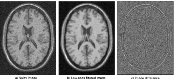
where the distance is calculated from a volume R computed as the subtraction of the original noisy volume u and the low pass filtered volume ψ(u) (using a 3x3x3 kernel) (see Figure 1). We have found experimentally that the minimum distance in this case is approximately equal to σ2 due to the removal of low frequency information and the application of the minimum operator.

This simple approach has two important benefits. On one hand, it allows finding more similar patches with the same structure but with different mean level compensating intensity inhomogeneities typically present on MRI data and on the other hand, overestimation of the noise variance will be minimized in cases with unique patches in the search volume. Thus, the adaptive filter proposed will set the parameter h2 equal to the minimum distance estimation as described in equation 10.

Adaptation to Rician noise

As previously noted, noise in magnitude MR images follows a Rician distribution. As consequence, the result of the weighted average will be biased due the asymmetry of the Rician distribution.

To avoid such bias, Manjón et al. (10) and Wiest-Daesslé et al. (13) recently proposed a Rician-adapted version of the original NL-means filter. These two approaches are very similar. Manjón approach yields a better global RMSE mainly due to a background overcorrection. Therefore, we have used the correction scheme proposed by Wiest-Daesslé that provides a better correction of the imaged object.

This Rician adapted filter removes bias intensity using the properties of the second-order moment of a Rice law. In fact, the second-order moment of a random variable X following a Rice distribution can be written as:

2 2 2

2

)

E(X

=

µ

+

σ

where σ is the variance of the Gaussian noise in the complex raw data. Based on this property of the Rice distribution, Wiest-Daesslé et al. (13) have proposed to restore the unbiased intensity value as:

















−

















=

∑

0

,

2

)

(

)

,

(

max

)

)(

(

NL

σ

w

x

x

u

x

x

u

The same approach can be applied to blockwise version of the NL-means filter before aggregating the estimations:

















−

















=

∑

0

,

2

)

(

)

,

(

max

)

)(

(

NL

σ

w

B

B

u

B

B

u

Then, the aggregation of the estimators can be performed as defined in Eq. (4).

In our case, as the estimation of σ is spatially dependent a low pass filter (kernel size 5x5x5) is applied to regularize the estimated bias volume to provide a more consistent correction. However, in the Rician case, the local noise estimation is underestimated on regions of low signal due the Rician nature of the noise. To correct such underestimation a correction factor was applied based on the local SNR as described by Koay et al. (22).

) ( ˆ2 2 SNR ξ σ σ = [14] where ξ(SNR) is defined as follows:

(

)

Here µ is the local mean, σ2 is the local estimation of the noise variance and σˆ2

is the corrected estimation in the Rician case. I0 and I1 are the 0th and 1st order

modified Bessel function of the first kind respectively.

Multiresolution Framework

As for all the denoising filters, the choice of the filtering parameters is crucial in NL-means-based restoration. The balance between structure preserving and noise removal is a difficult task. Different sets of parameters can be optimal for different space-frequency resolutions of the image. In Coupe et al. (9), a multiresolution framework based on wavelet transformation has been proposed to NL-means-based restoration of 3D MR images. This framework enables the procedure to implicitly adapt the filtering parameters according to the space-frequency resolution of the image. In the current approach we used the same strategy to optimize the denoising over all the frequencies of the image. Basically, this method is based on the application of the NL-means filter to the noisy volume with two different sets of parameters and mixing the results using different wavelet subbands from each restored volume. Details of the technique can be found in Coupé et al. (9).

The proposed approach in this paper is summarized on figure 2. As can be noted, no noise estimation (i.e. h parameter) is supplied to the method as this parameter is automatically estimated within the method. In all the experiments we set the ratio of the 3D search area M equal to 3 and the similarity 3D neighborhood have ratios of 1 and 2 for the multiresolution mixing. These parameters were found to be optimal in a previous work (9).

2.2. Evaluation Framework

Experimental data

To evaluate the proposed approach experiments were performed using the well-known Brainweb phantom (23-24). Three different image volume types were used in the evaluation, T1w, PDw and T2w with Gaussian and Rician noise levels from 1% to 15% of the maximum image intensity. Experiments were performed using both spatially homogeneous and inhomogeneous noise distributions. The Rician noise was built from white Gaussian noise in the complex domain:

)

(

)

(

)

(

)

(

I

x

=

I

x

+

β

x

η

x

η

(

x

)

~

N

(

0

,

σ

)

)

(

)

(

)

(

I

x

=

β

x

η

x

η

(

x

)

~

N

(

0

,

σ

)

where I0 is the “ground truth” and σ is the standard deviation of the added white

Gaussian noise. β(x_i) is the noise modulation function which is equal to one on the uniform case and spatially varying (range [1,3]) in the spatially dependent noise case. We used two example B modulation fields, one slow varying and one with fast transitions similar to those obtained on parallel imaging (See figures 3 and 4). Finally, the noisy image is computed as:

2 2

i

)

(

)

(

)

I(x

=

I

x

+

I

x

Quality measure

The Peak Signal Noise Ratio (PSNR) was used as quality measure and was computed as:

RMSE

255

Log

20

PSNR

=

where RMSE denotes the root mean square error estimated between the ground truth and the denoised image. For the sake of clarity, the PSNR values were estimated only in the region of interest (head tissues) obtained by removing the background (i.e. the label 0 of the discrete model in Brainweb).

In the case of the non-adaptive NL-means method the h2 parameter was set as the noise variance in the background (applied in the complex domain) as this is a common way to estimate the noise variance in clinical settings.

Therefore, during our experiment we have compared the following filter versions:

• NLM: Non Local Means Filter with Wavelet Mixing (9). This version includes blockwise approach, block preselection and wavelet mixing. The smoothing parameter was set to sigma (i.e. h2 = σ2).

• ANLM: Adaptive Non Local Means Filter with Wavelet Mixing. This version is similar to NLM filter but the smoothing parameter is locally adapted as described in Eq 10.

• RNLM: Rician Non Local Means Filter with Wavelet Mixing (13). This version include blockwise approach, block preselection, wavelet mixing and bias intensity correction as described by Wiest-Daesslé et al. The smoothing parameter was set to sigma (i.e. h2 = σ2).

• ARNLM: Adaptive Rician Non Local Means Filter with Wavelet Mixing. This version is similar to ANLM filter but with the corrected estimation of the local standard deviation of the noise σ as described in Eq 14.

In order to facilitate reproducibility of the presented experiments the source code of the filters are available at: http://webpage/page.html.

3. Results

Synthetic Data

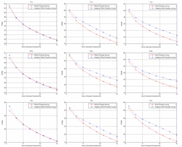
Comparison between the spatially-adapted and non spatially-adapted versions of the proposed filter can be found in Figs 5 and 6 for stationary and non-stationary simulated noise (Gaussian and Rician distributed noise). The main differences in the uniform noise case of the two compared versions are found for low levels of noise, where the local estimation of noise favours a better parametrization of the filter due to a small overestimation of the noise variance for such levels of noise yielding improved results. For non stationary noise the proposed filter outperforms the non adaptive version for all noise levels and modulation field shapes analyzed. In Figs 7 and 8, a visual example of the results obtained for both, slow and fast varying noise levels, with the different methods (9% Gaussian noise) are shown for visual inspection. As can be noticed, the proposed adaptive approach clearly outperforms the non-adaptive version in both cases while behaving similarly to the non-adaptive version on the case of spatially uniform noise (for both Gaussian and Rician distributed noise). In all cases, absolute value of the image differences did not show any anatomical information.

Real Clinical data

To evaluate the proposed approach on real clinical data, three datasets were used. The first one was obtained with a MP-RAGE T1 volumetric sequence (256x240x176 voxels with a voxels resolution of 1 mm3) acquired on a SIEMENS TRIO 3 Tesla scanner (Erlangen, Germany) using a GRAPPA acceleration factor of 2, TR=2300 ms, TE=2.9 ms, flip angle = 9º and TI = 900 ms. Result of the filtering of this dataset using the proposed method can be analyzed in Fig 9.

The second dataset was obtained with a TSE-FLAIR volumetric sequence (256x256x160 voxels with a voxels resolution of 0.94x0.94x1 mm) acquired on

a Philips Gyroscan 3 Tesla scanner (Netherlands) using a SENSE acceleration factor of 2, TR=14800 ms and TE=140 ms. This dataset was too noisy to be clinically useful but we use it here to better show the capabilities of the proposed approach on extremely noisy data. Result of the filtering of this dataset can be analyzed in Fig 10. As can be observed, the absolute value of the residuals of the filtering process clearly show the spatially varying noise pattern present in this data.

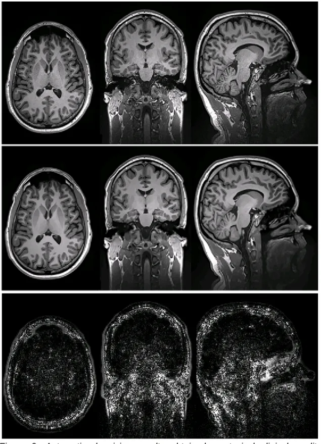
In order to show the performance of our method on classical 3D T1-w images (i.e. with stationary noise), the third dataset consisted in a MP-RAGE T1 weighted volumetric sequence acquired on a Siemens 1.5 Tesla Vision scanner (Erlangen, Germany). The acquisition parameters were, TR = 9.7 ms, TE = 4 ms, flip angle = 10º, TI = 20 ms, TD = 200 ms, 1x1x1.25 mm of voxel resolution. This dataset was downloaded from the fmri Data Center website (http://www.fmridc.org). Results of the filtering of this dataset can be analyzed in Fig 11. In this case, the proposed method also removed the noise successfully on a totally automatic manner showing no significant anatomical information on the image residuals. As can be observed in Fig 11, the background is masked due to the application of a defacer program. We have to notice here that due to this background extraction no noise variance estimation could be performed in such area as normally done for noise variance estimation in MRI. However, our method successfully denoised this data since it does not need such parameter as previously commented.

4. Discussion

To the best of our knowledge this is the first time that a method for spatially varying Rician noise filtering is proposed. Our approach has been demonstrated to produce similar results that the non-adaptive version of the filter for stationary noise without needing an explicit noise estimation (a small improvement is achieved for low noise conditions) and to clearly outperform the previously proposed non-adaptive version of NL-means filter for both spatially dependent Gaussian and Rician distributed noise.

Results over synthetic data showed an improved performance for different image types and levels of noise. The main benefit of the proposed filter is that it does not need any parameter related with the image noise level as it adapts itself to the quantity of noise present on the images locally. This filter can be applied to all kinds of images with either spatially homogeneous or inhomogeneous noise distribution. Furthermore, qualitative results on real clinical data are consistent with the results of synthetic data exhibiting no anatomical structures in the image residuals while being able to remove noise adaptively according to the local noise variance.

In conclusion, the obtained results suggest that the application of the proposed filter may benefit many quantitative techniques that rely on the good quality of the data. In this sense, applications such as segmentation, tractography or Relaxometry may take advantage from the enhanced data produced after the application of the proposed filter.

Acknowledgments

We would like to thank G. Garcia-Martí and Dr. Neda Bernasconi for providing the real clinical data used in this work and for their technical support.

References

1. Perona P, Malik J. Scale-Space and Edge Detection Using Anisotropic Diffusion. IEEE Transactions on Pattern Analysis and Machine Intelligence 1990; 12(7):629-639.

2. Gerig G, Kikinis R, Kubler O, Jolesz FA. Nonlinear anisotropic filtering of MRI data. IEEE Transactions on Medical Imaging 1992; 11(2):221-232.

3. Donoho DL, Johnstone IM. Ideal spatial adaptation via wavelet shrinkage. Biometrika 1994; 81:425–55.

4. Kuwamura S. Wavelet denoising for tomographically reconstructed image. Optical Review 2006; 13:129–37.

5. Nowak R. Wavelet-based rician noise removal for magnetic resonance imaging. IEEE Transactions on Image Processing 1999;8(10):1408–1419.

6. Pizurica A, Philips W, Lemahieu I, Acheroy M. A versatile wavelet domain noise filtration technique for medical imaging. IEEE Transactions on Medical Imaging 2003; 22:323–331.

7. Buades A, Coll B, Morel JM. A review of image denoising algorithms, with a new one. Multiscale Modeling & Simulation 2005;4(2):490–530.

8. Coupé P, Yger P, Prima S, Hellier P, Kervrann C, Barillot C. An Optimized Blockwise Non Local Means Denoising Filter for 3-D Magnetic Resonance Images. IEEE Transactions on Medical Imaging 2008; 27(4):425-441.

9. Coupé P, Hellier P, Prima S, Kervrann C, Barillot C. 3D Wavelet Sub-Bands Mixing for Image Denoising. International Journal of Biomedical Imaging 2008;Article ID: 590183. doi:10.1155/2008/590183

10. Manjón JV, Carbonell-Caballero J, Lull JJ, Garcia-Martí G, Martí-Bonmatí L, Robles M. MRI denoising using Non-Local Means. Medical Image Analysis 2008; 4(12):514-523.

11. Sijbers J, Den Dekker AJ, Van Audekerke J, Verhoye M, Van Dyck D. Estimation of the noise in magnitude MR images. Magnetic Resonance Imaging 1998;16(1):87–90.

12. Aja-Fernández S, Alberola-Lopez C, Westin CF. Noise and Signal Estimation in Magnitude MRI and Rician Distributed Images: A LMMSE Approach. IEEE Transactions on Image Processing 2008; 17(8):1383-1398.

13. Wiest-Daesslé N, Prima S, Coupé P, Morrissey SP, Barillot C. Rician noise removal by non-local means filtering for low signal-to-noise ratio mri: Applications to dt-mri. In: 11th International Conference on Medical Image Computing and Computer-Assisted Intervention, New York, USA, 2008. (pgs 171-179).

14. Pruessmann KP, Weiger M, Scheidegger MB, Boesiger P. SENSE: Sensitivity Encoding for Fast MRI. Magnetic Resonance in Medicine 1999; 42:952–962.

15. Griswold MA, Jakob PM, Heidemann RM et al. Generalized autocalibrating partially parallel acquisitions (GRAPPA). Magnetic Resonance in Medicine 2002;47:1202–1210.

16. Samsonov A, Johnson C. Noise-Adaptive Nonlinear Diffusion Filtering of MR Images With Spatially Varying Noise Levels. Magnetic Resonance in Medicine 2004;52:798-806.

17. Delakis I ,Hammad O, Kitney RI. Wavelet-based de-noising algorithm for images acquired with parallel magnetic resonance imaging (MRI). Physics in Medicine and biology 2007;52(13):3741-3751.

18. Mahmoudi M, Sapiro G. Fast image and video denoising via nonlocal means of similar neighborhoods. IEEE Signal Processing Letters 2005; 12(12):839–842.

19. Kervrann C, Boulanger J, Coupé P. Bayesian non-local means filter, image redundancy and adaptive dictionaries for noise removal. In: Proc Conf. Scale-Space and Variational Meth, Ischia, Italy, 2007.( pgs 520-532).

20. Brox T, Kleinschmidt O, Cremers D. Efficient nonlocal means for denoising of textural patterns. IEEE Transactions on Image Processing 2008; 17(7):1083– 1092.

21. Buades A, Coll B, Morel JM. Nonlocal Image and Movie Denoising. International Journal of Computer Vision 2008; 76(2):123-139.

22. Koay CG, Basser PJ. Analytically exact correction scheme for signal extraction from noisy magnitude MR signals. Journal of Magnetic Resonance 2006; 179: 317–322.

23. Kwan RK, Evans AC, Pike GB. MRI simulation-based evaluation of image-processing and classification methods. IEEE Transactions on Medical Imaging 1999; 18(11):1085–1097.

24. Collins DL, Zijdenbos AP, Kollokian V et al. Design and construction of a realistic digital brain phantom. IEEE Transactions on Medical Imaging 1998; 17(3):463–468.

Figures

Figure 1. Example of a noisy image and the difference image resulting from the subtraction of the low-pass filtered image. The image difference is used to estimate sigma by using the minimal distance computation between patches.

Figure 2. Diagram of the proposed method. Note that no parameters related the noise level (i.e. h parameter) has to be set in the proposed method.

Figure 3. Example of generation of a spatially slow varying noisy phantom. From left to right: Original noise free image (T1w), noise modulation map, resulting noisy image and absolute value of the applied non stationary noise (9% Gaussian distributed noise).

Figure 4. Example of generation of a spatially varying noisy phantom with fast noise level transitions. From left to right: Original noise free image (T1w), noise modulation map, resulting noisy image and absolute value of the applied non stationary noise (9% Gaussian distributed noise).

Figure 5. Gaussian denoising results. Left column: Comparison of the NLM and ANLM filters for different levels of homogeneous Gaussian noise. Center column: Comparison of the NLM and ANLM filters for different levels of slow varying spatially dependent Gaussian noise. Right column: Comparison of the NLM and ANLM filters for different levels of fast spatially varying Gaussian noise.

Figure 6. Rician denoising results. Left column: Comparison of the RNLM and ARNLM filters for different levels of homogeneous Rician noise. Center column: Comparison of the RNLM and ARNLM filters for different levels of slow varying spatially dependent Rician noise. Right column: Comparison of the RNLM and ARNLM filters for different levels of fast spatially varying Rician noise.

Figure 7. Denoising results of the NLM and ANLM filters applied to spatially slow varying Gaussian noise (9%). As can be noticed the NLM filter does not remove properly the noise in the central area of the image while our proposed approach is able to remove the spatially varying noise consistently in all the regions. The variable amplitude of the removed noise is easily noticeable in the absolute value of the residuals (e-f).

Figure 8. Denoising results of the NLM and ANLM filters applied to spatially fast varying Gaussian noise (9%). As can be noticed the NLM filter does not remove properly the noise in the central area of the image while our proposed approach is able to remove the spatially varying noise consistently in all the regions. The variable amplitude of the removed noise is easily noticeable in the absolute value of the residuals (e-f).

Figure 9. Automatic denoising results obtained on typical clinical quality magnitude MPRAGE images acquired using a GRAPPA acquisition (factor 2). From top to bottom: original noisy data, denoised data using the ARNLM method and the corresponding residuals.

Figure 10. Automatic denoising results obtained on very noisy images acquired using a SENSE acquisition (factor 2). From top to bottom: original noisy data, denoised data using the proposed approach and the corresponding absolute value of residuals.

Figure 11. Automatic denoising results obtained on images acquired using a conventional acquisition (no SENSE). From top to bottom: original noisy data, denoised data using the proposed approach and the corresponding absolute value of residuals.