Design of a novel test bench for induction heating load characterization

Design of a Novel Test Bench

for Induction Heating Load Characterization

by

Lisa Fernandez del Castillo

A.B. (Hons), Physics, University of Chicago (2012)

Submitted to the Department of Electrical Engineering and Computer Science

in partial fulfillment of the requirements for the degree of

Master of Science

at the

I

OF TECHNOLOGY

MASSACHUSETTS INSTITUTE OF TECHNOLOGY

June 2014

JUN 10

20M

@Massachusetts

Institute of Technology. All rights reserved.

LIBRARIES

Author ...

Signature redacted

...

U

Department of Electrical Engineering and Computer Science

May 21, 2012

Signature redacted

C ertified by ..

...

John G. Kassakian

Professor Emeritus of Electrical Engineering and Computer Science

Thesis Advisor

Signature redacted

A ccepted by ...

...

I

jLeslie

'

A. Kolodziejski

Professor of Electrical Engineering and Computer Science

Chair, Committee on Graduate Students

Design of a Novel Test Bench

for Induction Heating Load Characterization

by

Lisa Fernandez del Castillo

Submitted to the Department of Electrical Engineering and Computer Science

on May 21, 2014 in partial fulfillment of the requirements

for the degree of Master of Science

Abstract

Magnetic materials used in induction heating applications have nonlinear magnetic properties with respect to field strength and frequency, which can be effectively characterized using experimental techniques. To this end, we present a test bench inverter optimized for induction heating exper-imentation, capable of driving an inductive load across a 1-100 kHz frequency range with up to 2 kW power. Harmonic distortion of the inverter is minimized with a novel multilevel topology and modulation scheme, thus allowing near-sinusoidal excitations to be obtained at varying field strengths and frequencies. To demonstration the capabilities of the test bench, we characterize the power dissipation of a loaded induction heating coil across a range of frequencies and power levels.

Acknowledgments

This thesis would not have been possible without the support of a great many people.

First, I would like to express my deepest gratitude to my advisor, Professor John G. Kassakian, for his unfailing patience throughout my time here. His mentorship helped me not only to write this thesis but to develop as an electrical engineer. I am also so grateful to Dave Otten and Richard Zhang for their generous help with technical problems.

I would also like to thank all the wonderful people who have shaped my experience here at MIT: all the folks in LEES who have made doing research here so much fun, and everyone in the TCC who made MIT feel like home.

Finally, I would like to thank my family -my family at home in Chicago, my new family in Boston, and especially my wonderful husband- for all their love and support.

Contents

1

1.1 Magnetic Nonlinearities . . . . .

1.2

Thesis Objective & Approach

2 Background

2.1 Power Circuit Topology Review

2.1.1

Bridges . . . .

2.1.2

Resonant Inverters

.

. . .

2.1.3

Multilevel Inverters

.

. . .

2.2 Switching Method Review

.

. . .

2.2.1

Overview . . . .

2.2.2

Harmonic Cancellation .

2.3 Power Electronics Circuit Design

2.3.1

Switch Design . . . .

2.3.1.1

Switch Type . .

Switch Device . . . .

3 Circuit Design & Implementation 3.1 Power Circuit Topology Design . . . . .

3.1.1 Resonant Inverters . . . .

3.1.2 Multilevel Inverters . . . .

3.1.3 Cascaded Half-Bridge Full-Bridge

3.2 Circuit Implementation . . . . 3.2.1 Switching circuit . . . . 3.2.1.1 Switches . . . . 3.2.1.2 Thermal Considerations 3.2.2 Driving Circuit . . . . 11 12 13 15 15 15 17 17

20

20

20

25

3.2.2.1 3.2.2.2 3.2.2.3 3.2.2.4

Driver . . . .

Gate Circuit . . . .

4 Control Design & Implementation

4.1 Controls Design . . . . 4.2 Control Implementation . . . . 4.2.1 Overview . . . . 4.2.2 Program Design . . . .

5 Circuit Performance

5.1 Low to Medium Current Test

5.1.1 Experiment Design . .

5.1.2 Main Results . . . . .

5.1.3 Waveform Analysis . .

5.2 High Current Test . . . .

5.2.1 Experiment Design . . 5.2.2 Main Results . . . . . 5.2.3 Comparison of Voltage 5.2.4 Comparison of Harmon

. .. u. . . . .

.cs . .i. .. i. ...

. . . .

& Current Harmonics .

ics with Air-loaded Coil

6 Load Characterization Case Study

6.1 M ethod . . . .. ... .... . .... . . . . .. ... . . . .... . . . . 6.2 M agnetization Curves . . . .

7 Conclusion & Future Work A Transition Waveforms B Microcontroller Code C Circuit Details

C .1 Schem atic . . . . C.2 Selected Parts List . . . . D Fourier Transform Code

E Magnetization Curve Code Bibliography 36 37 37 38 39 39 39 41 41 46 46 46

50

67

70

73

.&

Pan-loaded Coil

List of Figures

1.1 Induction cooktop . . . . 12

1.2 Magnetization Curve of Iron. . . . . 13

2.1 Bridge Leg Configurations . . . . 15

2.2 Half-Bridge and Full-Bridge . . . . 16

2.3 Switch Diode . . . . 16

2.4 Standard Multilevel Inverters . . . . 18

2.5 Third Harmonic Cancellation Waveform . . . . 22

2.6 Time-Shifted Third Harmonic Cancellation Waveforms . . . . 22

2.7 Third and Fifth Harmonics Cancellation Waveform . . . . 23

2.8 Third and Fifth Harmonics Cancellation Fourier Transform . . . . 23

2.9 Thermal Circuit Model . . . . 26

2.10 Bootstrap Circuit . . . . 27

2.11 G ate C ircuit . . . . 29

3.1 Cascaded Half-Bridge Full-Bridge Inverter . . . . 30

3.2 CHBFB Output Voltage Levels . . . . 33

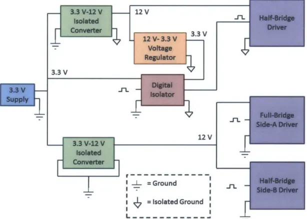
3.3 Diagram of the isolation and driving circuit power supply. . . . . 38

4.1 Ideal Voltage Waveform . . . . 41

4.2 Switching Cycle . . . . 43

4.3 Bridge Configuration Cycle . . . . 44

4.4 Control Signals . . . . 45

4.5 Control Diagram . . . . 45

4.6 Control Program Block Diagram . . . . 46

5.1 C ircuit B oard . . . . 51

5.2 Setup ... ... ... 52

5.3

53

5.4 Sample Low Current Waveforms . . . . 53

5.5 Low Current Fourier Transforms . . . . 55

5.6 Ideal and Achieved Voltage Waveforms . . . . 56

5.7 Difference Measurement at 42 A . . . . 57

5.9 Voltage Waveform and Difference Waveform Fourier Transform Comparison . ... . 6

5.10 Sample High Current Waveforms . . . . 61

5.11 High Current Fourier Transforms . . . . 62

5.12 Odd Harmonics Waveform Comparison . . . . 63

5.13 Odd Harmonics Voltage and Current Comparison . . . . 64

5.14 Odd Current Harmonics Pan-loaded and Air-loaded Comparison . . . . 65

6.1 Filtered Waveforms . . . . 67 6.2 Magnetization Curves . . . . 69 A. 1 Transition Waveforms . . . . 72 C.1 Microcontroller Schematic . . . . 78 C.2 Inverter Schematic 1 . . . . 79 C.3 Inverter Schematic 2 . . . . 80

C.4 Decoupling Capacitors Schematic . . . . 81

C.5 Miscellaneous Components Schematic . . . . 81 60

List of Tables

3.1

MOSFET Characteristics ...

...

35

4.1 PW M Settings .. . . ... ...

...

. . . . .. . . . .. . . . .. . . .. . . . .

48

Chapter 1

Introduction

Nonlinear magnetic properties often increase the complexity of applications involving magnetic

ma-terials. Many power applications use magnetic materials, most frequently as inductor and

trans-former cores. In these applications, the component is typically designed to avoid nonlinear magnetic

behavior, because nonlinear behavior tends to increase power loss in the magnetic material [1].

Induction heating is an interesting application because unlike inductor and transformer cores,

induction heating uses the magnetic material as the load. This is exemplified by the most common

domestic application of induction heating, the induction cooktop, as shown in Fig. 1.1. During

induction heating, an ac current creates an oscillating magnetic field that couples to the magnetic

material -the pan- and induces an electric field. The electric field gives rise to internal ac eddy

currents that generate ohmic heating in the pan. Typical induction cooktops operate under

condi-tions for which nonlinear magnetic behavior is assumed negligible [2, 3]. However, further research

is required to better understand how nonlinearities affect power dissipation in domestic induction

cooktop loads.

Experimental methods have great potential to increase our knowledge of the effects of magnetic

load nonlinearities in domestic induction cooktops. At present, there is no general theory that

can predict the magnetic properties of any material under any applied field. Experimentation,

on the other hand, can provide reliable information about magnetic materials for any condition,

provided we are capable of conducting the experiment. Specifically, experiments could allow for the

characterization of the impedance of nonlinear magnetic materials with respect to different induction

heating operation parameters.

To that end, in this thesis I provide an inverter test bench that is specialized for conducting

domestic induction cooktop load characterization experiments. In structure, the setup is comparable

to that of a commercial induction cooktop (see Fig. 1.1); it consists of a power electronics/control

circuit that drives an ac current through the a planar, spiral-shaped coil which heats the applied

pan via induction heating. However, the nature of the proposed load characterization experiments

place requirements on the inverter that require custom design features.

Figure 1.1: Typical domestic induction cooktop [4]. Our test bench has a similar structure, but our

bench lacks the glass separator and consists of one coil instead of four.

1.1

Magnetic Nonlinearities

A material's magnetic properties are described by its magnetization curve, such as the magnetization

curve of pure iron shown in Fig. 1.2, and different materials have different magnetization curves [5].

The magnetization curve can also be described in electrical terms; for an induction cooktop, the field

intensity H is proportional to the applied current through the induction coil I, and the magnetic

field B is proportional to the flux linkage A that gives rise to power loss in the magnetic material.

Using either of these metrics, the degree of nonlinearity is expressed by the slope of the curves:

the magnetic permeability p =

jB

in the B-H space, and the inductance L =

9

in the A-I space.

In linear materials, p and L are constant, and in nonlinear materials p and L are dependent on H

and I (respectively).

The magnetization curve illustrates four significant behaviors. First, the material saturates: for

large applied H, the change in the induced B approaches zero. Second, the material has saturation

remanence: after being saturated by a strong applied H, a non-zero B remains when H is no longer

applied. Third, the magnetization curve exhibits hysteresis: the B for a given H depends on the

history of the material. Fourth, the shape of the magnetization curve is frequency dependent.

In domestic induction cooktops, the most common load material is cast iron, which is an alloy

constituted of mostly iron with small (<5% by weight) amounts of silicon and carbon. Compared

to pure iron, cast iron saturates at a lower B and a higher magnetic permeability P

(using a

linear approximation) [1].1

For the purpose of load characterization experiments, it is important to note that the magnetic

properties are dependent on both the field intensity and on the frequency. Since the field intensity

is proportional to the supplied current, load characterization can be achieved by exciting the load

with a range of currents and frequencies.

'Another difference is that cast iron has a higher resistivity, which increases the ohmic heating in the material due to eddy currents [1]. This is beneficial for induction heating.

Fe(undeformed)

2

02Hz

-OJO H Z

-100

Hz

-200 Hz/

- -50 Hz

-1000

H

-2

-20

-15

-10

-5

0

5

10

15

20

H (kA/m)

Figure 1.2: Magnetization curves of pure iron at a variety of frequencies [6].

1.2 Thesis Objective & Approach

Based on the above discussion, the test bench required for the purpose of domestic induction cooktop load characterization must be able to excite inductive loads with a range of currents and frequencies. This places three requirements on the inverter. First, it must provide current excitations at a single frequency -current excitations that are near-sinusoidal, having low harmonic distortion. Generating a sinusoidal current waveform is achieved by generating a sinusoidal voltage waveform; the inductance in the load provides low-pass filtering on the current, reducing the higher harmonic content. Second, the inverter must provide these near-sinusoidal voltage and current excitations across a range of frequencies. Third, the inverter must provide a range of current levels at each frequency. This is achieved by providing a range of voltages.

To summarize, the test bench needs to drive inductive loads with near-sinusoidal voltage and current excitations across frequency and power level ranges broad enough for characterization of induction heating load nonlinearities. Additionally, the frequency and power level ranges should include the standard operating conditions of domestic induction cooktops, which are approximately

20-100 kHz and from 50 W-3.5 kW [7,

8].

Meeting these objectives requires the design of a custom inverter test bench. Specifically, the requirement that the inverter provide both high power and frequency flexibility prevents the use of commercial inverters that satisfy only one of these parameters. The inverters typically used to drive induction cooktops are inadequate for this application; commercial induction cooktops use resonant inverters, which achieve very high efficiency when operating near the resonant frequency but are not designed to operate across a range of frequencies [7, 8]. Inverters that are optimized for frequency flexibilities, such as function generators and impedance analyzers, do not output the high level of power needed to observe the nonlinearities of induction heating loads [9].

It is necessary, then, to design a new test bench in order to conduct induction heating load characterization experiments, and the purpose of this thesis is to meet that need. At the core of our

test bench is a novel inverter topology that is optimal for induction heating load characterization experiments: a cascaded half-bridge full-bridge (CHBFB) inverter, a hybrid proposed by David Otten of the topology in [10]. In order to generate the required high power, frequency flexibility, and near-sinusoidal voltage excitations, the CHBFB has been designed to generate voltage waveforms with low harmonic distortion -including cancellation of all voltage harmonics that are multiples of 2, 3, and 5 to below 3% of the fundamental- across 1-100 kHz at up to 2 kW.

The organization of this thesis is as follows: Chapter 2 overviews the background knowledge relevant to this research. Relevant inverter topologies and control methods are discussed, and an overview of power electronics circuit design is provided. Chapter 3 covers the circuit design and implementation. The novel CHBFB topology is introduced, and specifics concerning the circuit design and component selection are described. Chapter 4 covers the control design and implemen-tation. The basic program requirements and information flow are given, followed by the specifics of the control program. Chapter 5 presents the circuit performance. The test bench's ability to pro-duce near-sinusoidal waveforms across the stated frequency and power range is assessed. Chapter 6 presents an initial load characterization conducted with this test bench. Chapter 7 concludes with the results of this research effort and suggestions for future work.

Chapter

₂

Background

2.1

Power Circuit Topology Review

The inverter used in the test bench must generate near-sinusoidal waveforms across an inductive load

across a wide frequency and at up to kilowatt power levels. During the topology selection process

described in Chapter 3, Circuit Design & Implementation, several different types of inverters are

considered. This section describes these inverters.

2.1.1

Bridges

One of the building blocks of many common inverter topologies is the bridge leg. There are four

possible ways in which a bridge leg can be configured (see Fig. 2.1): high (in which the high-side

switch is on, and the low-side switch is off), low (in which the high-side switch is off, and the low-side

switch is on), open (in which neither switch is on), or shorted (in which both switches are on).

K

0

(a) High (b) Low (c) Open (d) Shorted

Figure 2.1: Possible bridge leg configurations.

Two of the simplest inverters are half-bridges, which consist of one bridge leg, and full-bridges,

which consist of two bridge legs. For both half- and full-bridges, normal operation consists of

switching between high and low bridge leg configurations. These topologies and their achievable

output voltage levels are shown in Fig. 2.2. Because the half-bridge consists of a single bridge leg,

it can only achieve two voltage levels: +Vdc when the bridge leg is high, and 0 when the bridge is

low. The full-bridge can achieve three voltage levels: +Vdc and -Vdc when the bridge legs are in opposite configurations (one high and the other low), and 0 when the bridge legs are in the same configuration (both high or both low).

Typically, the shorted and open bridge leg configurations are not used. The shorted bridge leg configuration is prohibited because that shorts the power supply, a phenomenon called shoot through. Additionally, the open configuration is avoided, because that leaves the output terminal floating. However, in order to avoid shoot through, it is common to implement a brief period in which the bridge leg is open during transitions between high and low configurations. If the load is reactive, it is necessary to provide a current path during this period. This is commonly done by placing diodes across the switches, such as MOSFETs' body diodes, as shown in Fig. 2.3.

Output VuAtge Levels of HNefBddg. bvenr

VdCC

V d c ...- .. ... ... ... ... ...

Vout

(a) Half-bridge (b) Half-bridge output voltage waveform

Output Vefta Leaw of Fufl-rdge kwener

(c) Full-bridge (d) Full-bridge output voltage waveform

Figure 2.2: Half- and full-bridges and their associated waveforms.

2.1.2

Resonant Inverters

Resonant inverters are a type of inverter in which the power output and efficiency are controlled by the frequency [1]. Although there are many different types of resonant inverter, the basic topology consists of a bridge leg that generates a square voltage waveform across a resonant network. When driving a reactive load, the load's reactance can be incorporated into the resonant network.

Resonant inverters are operated at maximum power output and efficiency at the undamped natural frequency, or resonant frequency, of the resonant network. Resonance is achieved at the frequency (wo) where the inductance (L) cancels the capacitance (C):

1 1

jwOoL +

=

woL - WOC

= 0

(2.1)

WO

This is the operating point of maximum power output and efficiency. As the frequency increases or decreases away from the resonant frequency, the power output and efficiency decrease. Near the resonance frequency, the dependence of the power on the frequency

I

Q

|2|

Q

Q

Resonant inverters have several key beneficial traits:

" High efficiency. If operated near the resonant frequency, resonant inverters are able to obtain

very high efficiencies.

" Power control. Since the power output is sensitive to frequency, adjusting the frequency can

be used as a means to control the power. The ability to make fine adjustment of the power level depends on

Q;

Q

" Low switch stress. Resonant inverters have two characteristics that limit the stress placed

on the semiconductor switches. First, because they generate sinusoidal waveforms, resonant inverters can achieve soft switching [11]. Second, the switching frequency is the carrier fre-quency; it is not necessary to use a high-frequency switching scheme such as PWM which causes increased switching losses in the devices. The low level of stress on the switches makes the resonant inverter topology suitable for high frequency applications.

The obvious disadvantage of resonant inverters is that they have limited frequency flexibility. Res-onant inverters do not operate well outside a given frequency window surrounding the resonance frequency.

2.1.3

Multilevel Inverters

Multilevel inverters are a family of inverters that produce stepped output voltage waveforms with three or more levels.

There are three standard types of multilevel inverters: diode-clamped, flying capacitor, and cascaded H-Bridge (CHB) as shown in Fig. 2.4. For the purpose of comparison, all three circuits in Fig. 2.4 are five-level inverters: an example of an output voltage waveform is shown in Fig. 2.4d.

V.

(a) Diode-Clamped (b) Flying Capacitor

V.

t

(d) Five-level Output Voltage Waveform

Figure 2.4: Five-level inverters using standard multilevel inverter topologies and an example five-level output voltage waveform [12].

The diode-clamped inverter consists of a ladder of switches held up by bulk capacitors and block-ing diodes (see Fig. 2.4a). The dc voltage is distributed evenly across the stack of bulk capacitors, and the switches are connected to the stack at different voltage levels. The output voltage, then, depends on the on/off configurations of the switches. In the five-level example, the bulk capacitors across the power supply each have a voltage of Vdc/4 across them, such that the possible output voltages are +Vdc, +Vdc/2,

0,

The flying capacitor inverter has a similar topology to the diode-clamped inverter (see Fig. 2.4b). However, instead of using blocking diodes, it uses additional storage capacitors to uphold the volt-age level between switches. Like the diode clamped inverter, the output voltvolt-age depends on the on/off configurations of the switches and in the five-level example, the possible output voltages are

+Vdc, +Vdc/2, 0, -Vdc/2, and -Vdc.

The CHB inverter is made of several single-phase, H-Bridge inverters connected in series (see Fig. 2.4c). Each H-bridge can produce at its output +Vdc/ 2, 0, or -VdC/2, depending on the state of the switches. When several single-phase inverters are connected in series, the output waveform is

-the sum of -the outputs of each individual inverter.

All multilevel inverter topologies share certain advantageous characteristics:

* Low harmonic content. Multilevel inverters generate output voltages with inherently low harmonic distortion; the total amount of harmonic distortion produced by a multilevel inverter decreases with the number of voltage levels [13]. This allows for the production of near-sinusoidal voltage waveforms even before any external filtering.

" Frequency flexibility. The output voltage waveform is entirely determined by the on/off

states of the semiconductor switches in the inverter; the number of output voltage levels, duration of levels, and waveform frequency are all controllable parameters. The frequency range, therefore, is limited only by the frequency range of the switches.

* Switching flexibility. Multilevel inverters can be controlled using either fundamental-frequency

switching methods or high-frequency switching methods depending on the requirements of the application [14].

However, the differences between the topologies give rise to advantages and disadvantages unique to specific topologies.

The diode-clamped inverter has two major drawbacks. The first is that it requires a large number of components per output voltage level compared to the CHB. This is illustrated by the example, in which eight switches, four capacitors, and six diodes of varying voltage rating are required to generate five output voltage levels. The second problem is bulk capacitor voltage unbalance. When creating a generic voltage waveform, the bulk capacitors do not necessarily have the same charging time, which causes them to charge to different voltages [12]. Because of this, the desired output voltage waveform is not produced by the inverter. Various approaches have been proposed to solve this problem, such as replacing the bulk capacitors by a controlled constant dc voltage source [12] and using an external switching circuit to balance the voltages [15].

The flying capacitor inverter has similar disadvantages to the diode-clamped inverter. Like the diode-clamped inverter, the flying capacitor inverter requires a large number of components per output voltage level compared to the CHB. In the example, eight switches and ten capacitors are required to generate five output voltage levels. In addition, voltage unbalance is a bigger problem in this topology than in the diode-clamped inverter because there are more capacitors that need to be balanced. This is countered by the fact that the flying capacitor inverter has more flexibility in the switching scheme than the diode-clamped inverter. Therefore, it is possible to balance the capacitors by using the proper switching scheme, but the design of the switching scheme becomes very complicated for inverters with many voltage levels [12, 13].

The CHB has several advantages over flying capacitor and diode-clamped inverters. It requires the fewest components per output voltage level [16]. Additionally, it does not require voltage balanc-ing [12]. The devices do not need to be rated for the full output voltage, and its modular structure simplifies repair and bypassing of faulty devices [16].

The main disadvantage of the CHB topology is that it requires multiple isolated voltage sources. This prohibits the use of many benchtop dc power supplies, which can exhibit problems with isolation due to parasitic capacitance across the transformers. This capacitance couples the output ground to

the supply line ground. Therefore, additional measures must be taken in order to ensure isolation, such as adding transformers between the voltage supply and inverting circuit [17, 18].

2.2

Switching Method Review

The switching method determines how a given power circuit topology is operated, and therefore it determines what output waveforms are generated. For this application, the switching method should generate a voltage waveform with low harmonic distortion. Selection of the optimal switching method depends on the circuit topology and application parameters. This section describes common

switching methods for multilevel inverters that may be considered for this application.

2.2.1

Overview

There are two categories of switching methods commonly used with multilevel inverters: high-frequency switching methods and fundamental-high-frequency switching methods [13].

High-frequency switching methods, which are based on either pulse width modulation (PWM) and space vector algorithms, are most suitable for low-frequency applications. While these meth-ods can produce a very accurate sinusoidal waveform, they are difficult to use in high frequency applications because they require the switching frequency to be much higher than the carrier fre-quency. PWM, for example, generally requires a switching frequency of at least ten times the carrier frequency. This is problematic because a switching frequency that high places additional stress on the devices that causes increased device power loss, requires additional heat sinking, and creates a higher risk for device breakdown.

On the other hand, fundamental-frequency switching methods require switching frequencies that are on the same order of magnitude as the carrier frequency, which is more favorable for high-frequency appliations. The three common varieties of fundamental-high-frequency switching methods are space vector control, nearest level control, and harmonic cancellation. Space vector and nearest level control methods both approximate the desired output voltage as the nearest achievable switching vector or output voltage achievable by the inverter. The harmonic cancellation method manipulates Fourier properties to minimize harmonic distortion in the output voltage waveform. Harmonic cancellation generally produces the lowest total harmonic distortion for inverters with five or fewer voltage levels, and space vector control and nearest level control work best for inverters that generate many output voltage levels [14].

2.2.2

Harmonic Cancellation

Harmonic cancellation is used to eliminate selected harmonics from the output voltage waveform of an inverter. In the stepped waveforms produced by multilevel inverters, the amplitudes of the harmonics inherently decay with increasing harmonic number. Therefore, in order to obtain an output voltage waveform from a multilevel inverter that is as sinusoidal as possible -that is, that has the lowest harmonic distorion as possible- it is necessary to cancel the lowest harmonics. Harmonic cancellation is typically only used for inverters with five or fewer levels because the number of equations that need to be solved to implement harmonic cancellation increases with the number of

voltage levels [141. This section considers a five-level inverter, for which it is possible to cancel all harmonics that are multiples of 2, 3, and 5 (all 2n, 3n, and 5n harmonics).

The prinicipal behind harmonic cancellation is that every waveform can be decomposed into a sum of sinusoids:

f

(t)=

+ E

an

sin

+

E

b, cos

(2.3)

an

=

f

b =

f (t) cos (nwt)

(2.5)

Based on this property, some useful generalities may be observed. First, if the waveform f(wt) is odd, then

T

bn

2

J

f

&(t) cos (nrwt) = 0

(2.6)

0

and so all odd functions have no cos harmonics. Similarly, all even functions have no sin harmon-ics. Finally, it can also be shown that half-wave symmetric waveforms have no even harmonics

(a2k and b2k = 0 for all k). Therefore, in order to cancel all cos harmonics and all even sin harmonics

from the output voltage, we will generate an odd half-wave symmetric waveform. The resulting waveform is composed solely of a,, a3, a5, etc.

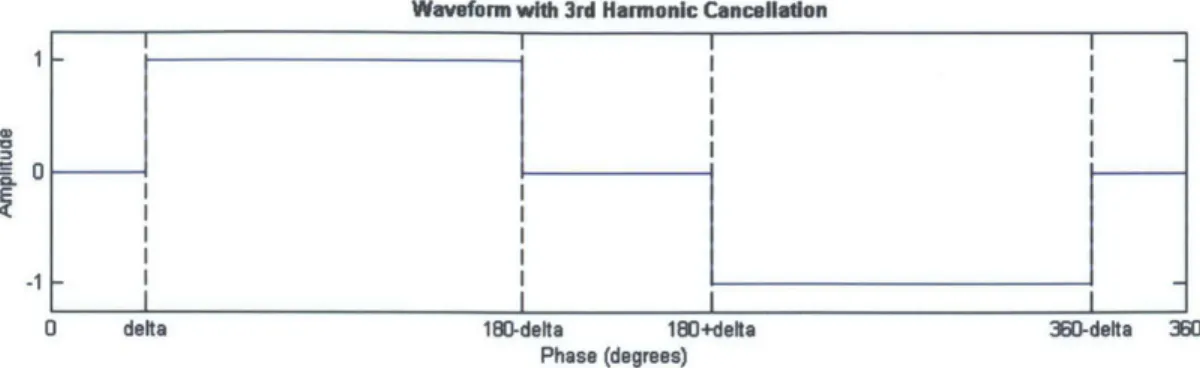
Harmonic cancellation of a given harmonic (an or bn) is achieved by setting the durations of the voltage levels such that the amplitude of that harmonic across the cycle equals zero. For example, consider the three-level waveform shown in Fig. 2.5. Because it is odd and half-wave symmetric, all cos and even harmonics are cancelled. The amplitude of the nth harmonic is

180o6 360*-6

an

J

V

6 1800+6

If 6 is set such that the integrals are equal to zero, then an = 0 as well as all multiples of an

(2an, 3an, etc.). Since an odd, half-wave symmetric waveform, is already free of all even harmonics, the largest present harmonic is the third. This harmonic can be cancelled by setting a =30 '. In this case, all cos harmonics, even harmonics, and harmonics that are multiples of 3 (3, 6, 9, etc.)

are cancelled, and we can write the waveform as:

00

f

an sin (nwt)

n=1,5,7,11,...

0

-1

Waveform with 3rd Harmonic Cancellation

_ -- __ _ _ _ _ _ _ _

I_

a delta 180-delta 180+defta

Phase (degrees)

3WD-delta 350

Figure 2.5: Three-level voltage waveform with cos, 2n, and 3n harmonics cancelled.

harmonics (5, 10, 15, etc.). Although the waveform that provides for cancellation of all cos, 2n, 3n,

and 5n harmonics can be calculated directly using the method shown above, the extra voltage levels

complicate the procedure. However, the required waveform can easily be derived by considering the

five-level waveform as the sum of two time-shifted versions of the three-level waveform in Fig. 2.5.

Like the original, the time-shifted waveform has no third harmonic; a linear operation (time-shifting)

cannot reintroduce a harmonic that does not exist in the original waveform. This is shown in Fig. 2.6.

osiglal

Waveform

I

0

3M+defta [~~I 3D+de i 150+dek I 210+detaI_ _ _ _ _ Phase (degrees)

Weveesm wih 54. Hrmane Concefela

330+deka 30 30+dete 10 150+kdea 210 210+dea 3Mdea

Phase (degrees)

Figure 2.6: Time-shifted waveforms with cos, 2n, and 3n harmonics cancelled; and the summed

waveform with cos, 2n, 3n, and

5n

harmonics cancelled.

The original waveform can be written as the sum in (2.8), and therefore the time-shifted waveform

can be written

an sin (nw(t

At))

fn(t - At) =

,

1

(2.9)

Therefore, the nth harmonic of the sum of the two waveforms is

fn(t)

+

fn(t

At)

=

an

sin

(nwt)

an

sin

(nwt

nwAt)

Cancellation of the nth harmonics is achieved when nwAt =

such that

fn(t)

fn(t

At)

an sin (nwt)

an sin (nwt

nwAt) =

0

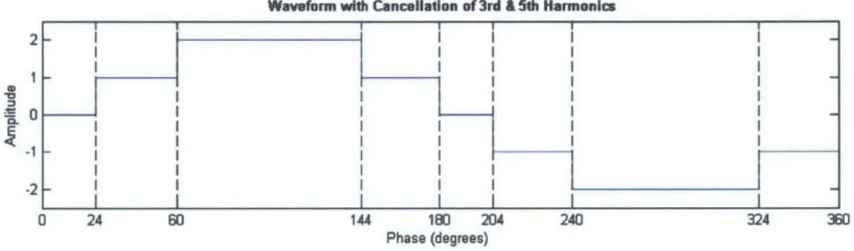
Therefore, cancellation of the 5th harmonics is achieved by setting wAt

is shown in Fig. 2.7.

Waveform with Cancellation of 3rd

A 5th

Harmonics

-2 0 24 60 144 180 204 Phase (degrees) 240

(2.10)

(2.11)

This waveform

Figure 2.7: Waveform with no cos, 2n, 3n, or

5n

harmonics.

The harmonic content of this waveform is shown by taking the Fourier transform, which is shown

in Fig. 2.8. The 2n, 3n, and 5n harmonics are cancelled to below

of the fundamental, while

the 7th and 11th harmonic are both about 10-1 of the fundamental (see Fig. 2.8). The large value

of the 7th and 11th harmonics is expected because the switching scheme was not designed to cancel

them. The non-zero magnitudes of the 2n, 3n, and

5n

harmonics is due to the machine epsilon of

the computation:

is the rounding error for floating point numbers. Therefore, these values

are approximately zero, confirming that the ideal waveform achieves cancellation of all 2n, 3n, and

5n

harmonics.

1010

10-2

0

FFT

N

or

I

I

I

1

2

3

4

5

6

Harmonic number

Figure 2.8: Fourier transform

the fundamental is 1.

)

7

8

9

10

11

of the ideal voltage waveform, normalized such that the amplitude of

I T - I I I I I - I I I I - I I I I CD N 0

z

2.3

Power Electronics Circuit Design

Merely choosing the correct circuit topology and switching method is not enough to create a suc-cessful inverter. Careful design of the circuit board is also crucial to building a well-functioning inverter. This section reviews two key design aspects that must be considered when designing a power electronics circuit: the switches and the driving circuit.

2.3.1

Switch Design

The switches are one of the most important components of any power electronics circuit. They are the devices that allow the circuit to operate in different modes, without which the circuit could not function as a power dc-ac inverter. Switch design consists of three processes: selection of the switch type, selection of the switch, and design of the thermal system needed to keep the switches from overheating.

2.3.1.1 Switch Type

Determining which type of switch to use is a process of comparing the specific application needs with the capabilities of the different types of switches.

There are two categories of switches: passive and active. A passive switch, such as a diode, cannot be user-controlled but is controlled by conditions in the circuit. An active switch, such as a transistor, are user-controllable. In power applications, the most commonly used transistors are the power metal-oxide-semiconductor field-effect transistor (power MOSFET) and the insulated-gate bipolar transistor (IGBT). For MOSFETs and IGBTs, the voltage at the gate determines whether the drain-source and collector-emitter channels (respectively) conduct current or block voltage.

Due to structural differences, power MOSFETs and IGBTs are preferrable under different condi-tions.1 Power MOSFETs are more commonly used for applications requiring low voltages (< 200 V), low powers (<~500 W), high frequencies (>-200 kHz), long duty cycles, and big load variations. IGBTs, on the other hand, are typically used for applications requiring high voltages (>-1000 V), high powers (>-5000 W), low frequencies (<-20 kHz), short duty cycles, small load variations, and high temperatures [20].

In addition, both MOSFETs and IGBTs can be categorized by their dominant current carrier: electrons (N-type) or holes (P-type). Electrons have a higher mobility than holes. Since the resistiv-ity of a material is inversely proportional to the carrier mobilresistiv-ity, N-type devices tend to have lower resistivities and are more commonly used.2

2.3.1.2 Switch Device3

The switches must provide good performance while meeting the voltage and current ratings of the application. The performance of the switches can be measured with respect to three criteria:

on-1A thorough discussion of the physical differences between the power MOSFET and IGBT is not necessary for this

work, but one can be found in [19].

2

Again, an in-depth comparison of the n-type and p-type transistors is not necessary for this work, but one can be

found in [19].

3

N-type Power MOSFETs are considered throughout the rest of this chapter, since these are the devices used in the test bench.

state resistance, switching speed, and thermal characteristics. All of these criteria are described

by parameters that are included in devices' data sheets, making it easy to select the device that is

optimal for a specific application.

It is critical to have a low on-state resistance in order to minimize power losses during conduction. The on-state resistance is the resistance of the switch when it is conducting current. This device characteristic is dependent on many operation parameters such as the device's gate-source voltage, drain-source current, and temperature.

In addition, having a high switching speed is important for two reasons. First, when the switch is transitioning between the on- and off-states it is partially conducting, such that it has both a voltage and current across it, resulting in power losses in the device. By maximizing the switching speed of the device, the switching loss is minimized. Second, the devices selected must be capable of switching at the required frequency of the application. The device's rise and fall times specify how quickly its drain-source voltage can change between the on- and off-states. In addition, the device's gate charge determines how quickly it responds to control signals at its gate. A switch with a small gate charge will charge and discharge more rapidly than a switch with a large gate charge, allowing it to respond more quickly to control signals.

Finally, devices with favorable thermal characteristics place low requirements on the thermal system. The two key thermal parameters of a MOSFET are its maximum junction temperature and the thermal resistance. The maximum junction temperature is the maximum temperature that the interior of the switch device can reach without breaking down. The thermal resistance measures how much the temperature of the device increases when it generates heat. It is beneficial to use devices with high maximum junction temperatures and low thermal resistances.

2.3.1.3 Thermal Considerations

Thermal considerations play an important part in the switch design. During operation, each

MOS-FET dissipates power, causing its temperature to rise. If the temperature increases beyond its

rating, the device breaks down. In order to avoid this, a heat sink must be attached to each device to keep it cool.

The loss in a MOSFET can be approximated as the sum of the conduction losses and the switching losses [11:

Pdis, ~~

conduction losses + switching losses - (Irm3Rds,on)

(2.12)

where Irm, is the rms drain current, Rd8,, is the on-resistance, VDS is the drain-source voltage,

f

is the frequency, and tr and tf are the rise and fall times of the drain-source voltage.

The heat resulting from the power dissipation in the MOSFET is removed via an attached heat sink. The heat sink is usually attached to the MOSFET package using thermally-conductive paste or a thermally-conductive pad. The necessary cooling is described by the thermal circuit in Fig. 2.9. In this figure, Pdis, is the power dissipated by the MOSFET, Tj is the temperature of the MOSFET junction, Rjc is the thermal resistance between the MOSFET junction and case, Rc, is the thermal resistance between the MOSFET case and the heat sink, R,, is the thermal resistance between the heat sink and the ambient air, and Ta is the ambient temperature. A standard design practice

is to leave a 20*C safety margin between the maximum rated device junction temperature and the maximum temperature reached during device operation. Therefore, the maximum allowable thermal resistance of the heat sink can be calculated:

_(T. 2 00 C -Ta)R sa = _ -_00C-__

Rjc

Ti

Rjc

Pdiss

RCS

Rsa

Ta

Figure 2.9: Thermal circuit describing the heat caused by power dissipation in MOSFETs.

2.3.2

Driving Circuit Design

The driving circuit consists of the devices that ensure that the switches turn on and off correctly.

The key processes involved in driving circuit design are selection of the high-side driving method,

driver selection, and gate circuit design.

2.3.2.1

High-side Driving Method

Special techniques must be employed to drive the high-side N-type MOSFETs. The gate voltage

must be higher than the drain voltage when the MOSFET is in the linear region. This is not an

issue for low-side MOSFETs because their sources are tied to circuit ground, and when in the linear

region their drain voltage is low. However, the source voltage of high-side MOSFETs is elevated

relative to circuit ground -it is tied to the drain of the low-side MOSFET- and therefore the drain

voltage can often be too high to feasibly allow for a ground-referenced gate signal.

One of the most popular ways to drive high-side N-type MOSFETs is charge pumping. A charge

pump is a type of dc-dc converter that uses energy storage elements to generate voltage pulses of

higher magnitude than the gate drive supply voltage. Although there are many varieties of charge

pump circuits, the most common type of charge pump used for high-side driving is the bootstrap

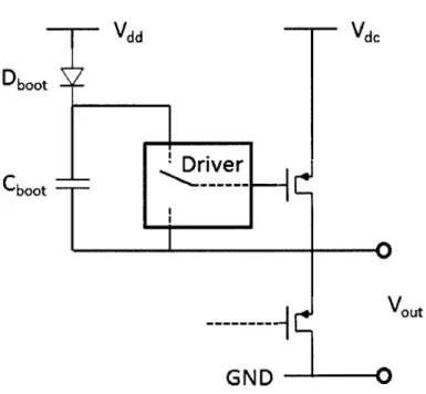
circuit. The basic bootstrap circuit is shown in Fig. 2.10. When the driver provides a low signal,

it ties the gate of the high-side MOSFET to its source. This turns off the MOSFET. During this

stage of the cycle, the bootstrap capacitor charges. During the second stage of the cycle, the driver

provides a high signal, tying the gate of the high-side MOSFET to the charged bootstrap capacitor.

During this stage of the cycle, the bootstrap capacitor discharges to drive the high-side MOSFET,

and the magnitude of the gate signal is the voltage across the bootstrap capacitor.

Vdd

Vdc

Dboot

-SDriver

I:

A

out

GND

0

Figure 2.10: Bootstrap circuit.

The bootstrapping method of driving the high-side switch relies upon proper selection of the

bootstrap diode and capacitor. The range of adequate capacitance of the bootstrap capacitor is

bounded by two criteria: it must be big enough to provide the required gate voltage, and it must be

small enough to fully charge when the high-side switch is turned off [21].

The minimum capacitance required to ensure that the bootstrap capacitor can drive the

MOS-FET gate high is determined by the relation C

=

Q:

V.

QG +

+

CBS,min =

AV(2.14)

where

is the minimum required bootstrap capacitance, QG is the high-side MOSFET's gate

charge, QRR is the bootstrap diode's reverse recovery charge,

is the bootstrap diode's reverse

leakage current,

is the upper supply quiescent current,

f

is the minimum switching frequency,

and AV is the allowed change in voltage across the capacitor during discharge.

On the other hand, the bootstrap capacitor must be small enough so that it can be fully charged

up during the off-time of the high side MOSFET. Again, this is determined by the relation C = Q:

CBSmax - Imax x Atmin Imax (2.15)

AV

AV

where Imax is the maximum current supplied by the bootstrap diode; Atmin is the shortest amount

of time the capacitor will have to charge, or ~

-1; and again, AV is the allowed change in voltage

Based on the above discussion, there are two requirements for the bootstrap diode. First, it

should have low reverse recovery charge and leakage current to minimize the total charge that the

capacitor needs to provide. Second, it should have a high maximum current to facilitate fast charging

of the bootstrap capacitor.

2.3.2.2 Driver

The driver is the main component of the driving circuit. It receives the low-current digital

con-trol signals and delivers them to the MOSFET gates with enough current to produce clean on/off

transitions.

The selected driver must be able to meet several requirements. First, it must be able to source

and sink enough current to turn the MOSFETs on and off at the required speed. It must provide

gate signals that are high enough to bias the MOSFET into the linear region where the on-state

resistance is low. It must generate the desired gate signals based on input control signals. It must

isolate the signal to the high-side switch to have a ground reference of the switch's drain. Finally,

it may have a mechanism for preventing shoot through -a spike of current "shooting through" the

circuit due to a shorted power supply, which usually occurs when a bridge leg is shorted briefly

during the transition between high and low configurations.

Shoot through prevention is an optional feature for gate drivers because it may also be achieved

in the controls. The advantages and disadvantages of preventing shoot through with the driver

versus in the controls is case specific based on the characteristics of the particular driver and control

method used. Many commercial drivers and control devices have built-in shoot through prevention

that are reliable and easy to implement. When using a device with built-in shoot through prevention,

it is often simplest to use this option rather than implementing it using external circuit devices or

an additional control program.

There are many options for selecting a driver to meet these requirements. The first option is

to build a custom driver. This option provides the most control over the driving circuit. The

chief drawback is the additional design complexity; driver design is not a trivial task, especially if

features such as shoot through prevention or undervoltage protection are incorporated. Unless the

application has a non-standard driving requirement, it is generally simpler to use a commercially

available driver.

Among commercial drivers, there remain many options to choose from. Particularly, there are two

categories of commercial drivers: single-output drivers, for driving high-side or low-side switches,

and multi-output drivers, for driving both low- and high-side switches. The main advantage of

using single-output drivers is the ability to achieve more compact driving circuits, which improves

switching performance. On the other hand, the benefit of using multi-output drivers is the ability

to drive an entire bridge using a single driver chip. Most commercially available drivers use the

bootstrapping method to drive the high-side switch.

2.3.2.3 Gate Circuit

Finally, conditioning of the gate signal is required in order to achieve clean load voltage transitions.

This is because the load voltage waveform depends on the drain-source waveforms across the

MOS-FET switches, and each MOSMOS-FET's drain-source waveform depends on its gate-source waveform.

Fast drain-source high/low transitions cannot be achieved without fast gate-source transitions, and

the amount of drain-source overshoot and ringing is strongly dependent on the amount of gate-source

overshoot and ringing. In addition, it is necessary to have fast MOSFET turn-off transitions in order

to avoid shoot through.

Therefore, the gate signal is required to have acceptable gate-source rise and fall times and

drain-source overshoot. The speed of the gate-source transition is typically limited by how quickly

the gate current can charge or discharge the gate capacitances [22]. Although this is predominantly

determined by the driving circuit, devices in the gate path of the MOSFET can alter gate-source

rise and fall times. Drain-source overshoot and ringing is caused by the inherent gate-source and

drain-source capacitances of the MOSFETs; resistance and inductance due to other circuit elements;

and parasitic capacitance, resistance, and inductance due to layout [19].

A standard method for gate-signal conditioning is the placement of a resistor and diode between

the driver and MOSFET in the configuration shown in Fig. 2.11. The gate resistor damps response

to an input signal, which causes slower transition times but smaller overshoot and ringing. The

additional placement of a gate diode allows for a fast gate-source voltage fall time, reducing the risk

of shoot through.

D9

R

Chapter 3

Circuit Design & Implementation

A test bench is needed that can provide near-sinusoidal voltage and current excitations across an

inductive load across a wide frequency and at up to kilowatt power levels. The novel cascaded

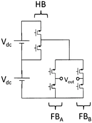
half-bridge full-half-bridge (CHBFB) inverter topology, shown in Fig. 3.1, is optimal for meeting these needs.

This chapter describes the advantages of this topology, how it operates, and how it was implemented

to meet the particular requirements of this work.

HB

VdC

FBA

_FBB

3.1

Power Circuit Topology Design

The topology of the power circuit must be optimal with respect to its ability to generate near-sinusoidal waveforms across an inductive load across a wide frequency and power range. This section describes the topology selection process.

3.1.1

Resonant Inverters

Since commercial induction cooktops use resonant inverters, it would seem reasonable that this topology could be adapted for induction heating load experimentation. However, this is not an ideal strategy because resonant inverters lack the frequency flexibility needed to conduct load characteri-zation experiments.

Commercial induction cooktops use resonant inverters because maximizing the efficiency is crit-ical for that application, but frequency flexibility is relatively unimportant. The inductance of induction heating loads is incorporated into the resonant network so that the system can achieve efficiencies of over 98% [8]. Peak power and efficiency are achieved by operating near the resonant frequency, and the power level can be lowered by moving the operating frequency away from res-onance [7, 8, 23]. Resonant inverters are ideal for meeting the objectives of commercial induction cooktops.

However, because resonant inverters are designed at a fixed frequency with only slight variation, they are incapable of driving an inductive load across broad frequency and power ranges. Although resonant inverters are capable of driving an inductive load across a wide frequency range, doing so would result in a tremendous reduction in the output power capability of the inverter. Llorente et al. have shown that even varying the frequency by a factor of two reduces the power output to less than 40% of peak output for the most common induction cooktop resonant inverter topologies [8]. Therefore, the standard resonant inverter topology is inadequate for this work.

Although it is possible to adapt resonant inverters to operate across a range of frequencies, doing so requires significant additional circuit complexity. Puyal et al. have built a series-resonant half-bridge inverter module for the purpose of inductive load characterization [9]. Although based on a resonant inverter topology, their inverter achieves frequency flexibility by modifying the resonant frequency using a large, adjustable capacitor bank. This allows the inverter to sweep across a range of frequencies while always operating near the resonant frequency. However, the design and assembly of the capacitor bank is not trivial. Therefore, although the frequency-controllable resonant inverter topology demonstrated by Puyal et al. is a feasible method of achieving our goals, from a design perspective it is not ideal.

3.1.2

Multilevel Inverters

Multilevel inverters meet the needs of the test bench:

* Inductive Loads. Multilevel inverters are capable of driving inductive loads, in which the

impedance angle is between 0'-90'. This is demonstrated by their common use as reactive power compensators and induction motor drives [12].

* Near-sinusoidal voltage excitations. The amount of harmonic distortion generated by a

multilevel inverter decreases with the number of voltage levels.

* Frequency Range. Multilevel inverters are able to operate across a wide range of frequencies

because the output voltage waveform is entirely determined by the on/off states of the semi-conductor switches in the inverter; the number of output voltage levels, duration of levels, and waveform frequency are all controllable parameters. The frequency range, therefore, is limited only by the frequency range of the switches.

* Power range. Multilevel inverters are more than capable of operating at power levels in the

kilowatt range. Multilevel inverters have been used extensively since the 1990's for medium-voltage high-power applications in the kilovolt, kilowatt range and higher [12, 24J.

However, as discussed in Chapter 2, Background, each of the three standard multilevel topologies has certain disadvantages that require additional circuit complexity to overcome. Therefore, while any of the three standard multilevel topologies are adequate, none are ideal. Diode-clamped and flying capacitor multilevel inverters both require a large number of components per output voltage level and have problems with device voltage balance. While CHB inverters do not have these issues, they require two isolated dc sources. Although none of these issues render the inverters insufficient for the proposed inductive load experiments, they do require additional complexity in the circuit, the switching scheme, or both. A more optimal topology is wanted that can meet the needs of this application without a large number of components, without issues related to voltage balancing, and without the need for isolated supplies.

3.1.3

Cascaded Half-Bridge Full-Bridge

A hybrid class of multilevel inverters called the cascaded multilevel inverter (CMI) provides the

advantages of the standard multilevel inverters without the problems associated with the diode-clamped, flying capacitor, and cascaded H-bridge topologies. The CMI consists of two- or three-level inverters, such as half- and full-bridges, cascaded together in series. Specifically, a CMI topology we

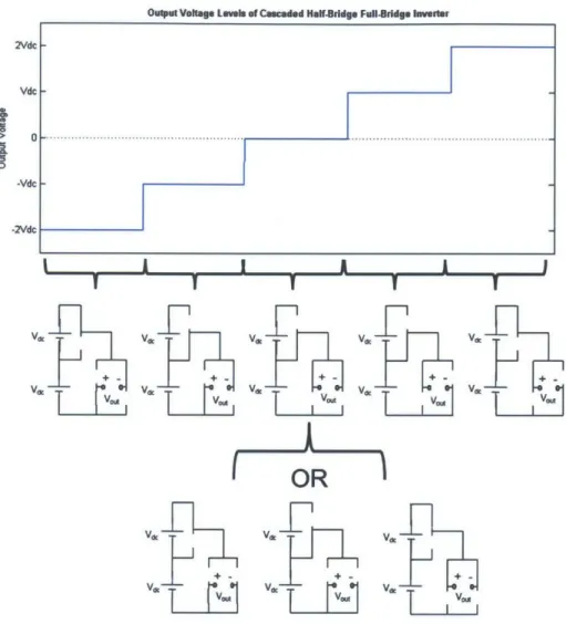
call a cascaded half-bridge full-bridge (CHBFB) inverter is ideal for the needs of this work. The CHBFB inverter consists of a half-bridge in series with a full-bridge, as shown in Fig. 3.1. The full-bridge is capable of achieving output voltages of zero and ± the rail voltage. The half-bridge sets the full-bridge's rail voltage to either Vdc or 2Vdc. Therefore the possible output voltage levels are 2Vdc, Vdc, 0, -Vdc, or -2Vdc. The bridge

leg

The CHBFB surpasses the performance of the standard multilevel topologies in several respects. First, it produce a five-level output voltage waveform with only six switches, compared to the eight or more required by the three standard multilevel topologies. In addition, it does not require additional blocking diodes, flying capacitors, or isolated dc sources. Although it does use two sources, they are connected in series and do not require isolation. Thus, it is capable of meeting the needs of this application with minimal circuit complexity.

In addition, the flexibility in the zero-state configuration allows for the minimization of the number of high/low bridge changes in the cycle, which reduces the demands on the controls and