Multiscale approach for the pore space characterization of gas shales

(1)

HAL Id: tel-02536342

https://tel.archives-ouvertes.fr/tel-02536342

Submitted on 8 Apr 2020

HAL is a multi-disciplinary open access archive for the deposit and dissemination of sci-entific research documents, whether they are pub-lished or not. The documents may come from teaching and research institutions in France or abroad, or from public or private research centers.

L’archive ouverte pluridisciplinaire HAL, est destinée au dépôt et à la diffusion de documents scientifiques de niveau recherche, publiés ou non, émanant des établissements d’enseignement et de recherche français ou étrangers, des laboratoires publics ou privés.

Multiscale approach for the pore space characterization

of gas shales

Natalia Matskova

To cite this version:

Natalia Matskova. Multiscale approach for the pore space characterization of gas shales. Earth Sciences. Université de Poitiers, 2018. English. �NNT : 2018POIT2276�. �tel-02536342�

(2)

THESE

Pour l’obtention du Grade de DOCTEUR DE L’UNIVERSITE DE POITIERS (Faculté des Sciences Fondamentales et Appliquées)

(Diplôme National - Arrêté du 25 mai 2016) Ecole Doctorale : Gay Lussac

Secteur de Recherche : Terre solide et enveloppes superficielle Présentée par :

Natalia Matskova

************************

APPROCHE MULTI-ÉCHELLE POUR LA CARACTÉRISATION DE L'ESPACE POREUX DES RESERVOIRS PETROLIERS ARGILEUX NON

CONVENTIONELS ************************ Soutenue le 06/07/2018 devant la Commission d’Examen

************************

JURY

Rapporteur : Laurent Michot (Directeur de recherche CNRS) Rapporteur : Professeur Yves Geraud

Examinatrice : Docteur Claire Fialips Examinatrice : Professeur Patricia Patrier Directeur de Thèse : Professeur Philippe Cosenza

Co-directeur de Thèse : Docteur Dimitri Prêt Co-directeur de Thèse : Docteur Stéphane Gaboreau

(3)

(4)

M

ULTISCALE APPROACH FOR THE PORE SPACE

CHARACTERIZATION OF GAS SHALES

(5)

(6)

(7)

(8)

Abstract

Gas shale reservoirs are characterized by pore systems, associated with a heterogeneous spatial distribution of mineral and organic phases at multiple scales. This high heterogeneity requires a multi-scale & multi-tool approach to characterize the pore network. Such an approach has been developed on 7 cores from the Vaca Muerta formation (Argentina), which belong to areas with various hydrocarbon maturities, but with comparable mineral compositions. 3D µtomography and quantitative 2D mapping of the connected porosity by autoradiography have been applied at the core scale, localize and analyze the spatial heterogeneities, and to identify similar homogenous areas for localizing comparable sub-samples.

The correlative coupling of various techniques was applied to achieve quantitative balance of porosity and pore size distribution, from mm to nm scales on representative sub-samples and for the first time, on preserved blocks rather than crushed powders, even for nitrogen gas adsorption experiments. Results of autoradiography are in very good agreement with other total bulk porosities, indicating that all pores are connected and accessed by the 14_{C-MMA used for impregnation. Decreased total porosity and pore}

throat/body sizes were also observed as organic matter maturity increased.

An innovative approach for electron microscopy images acquisition and treatment provided large mosaics, with the distribution of mineral and organic phases at the cm scale. The correlative coupling with the autoradiography porosity map of the same zone, revealed the spatial correlations between mineralogical variations and porosity.

Key words: Earth science, clay, scanning electron microscopy, x-ray tomography, unconventional reservoirs, shale oil and gas, porosity, correlative imaging.

(9)

Résumé

Les réservoirs pétroliers argileux sont caractérisés par des systèmes de pores associés à une distribution spatiale hétérogène à plusieurs échelles des phases minérales et organiques. Cette hétérogénéité nécessite une approche multi-échelle et multi-outils pour caractériser le réseau de pores. Une telle approche a été développée grâce à la sélection rigoureuse de 7 carottes issues de la formation de Vaca Muerta (Argentine), avec différentes maturations d'hydrocarbures mais des compositions minérales comparables. La tomographie RX 3D et la cartographie de la porosité par autoradiographie ont révélé les hétérogénéités à l'échelle des carottes, et permis d'identifier des zones homogènes pour le prélèvement de sous-échantillons comparables et représentatifs.

Le couplage corrélatif de différentes techniques a permis d'atteindre un bilan quantitatif de la porosité / tailles de pores et pour la première fois, sur des blocs non broyés, notamment pour les expériences d'adsorption d'azote. Les résultats d’autoradiographie sont en accord avec les autres méthodes, indiquant que tous les pores sont connectés et accessibles par la résine d’imprégnation. Une diminution de la porosité totale ainsi que des tailles de pores a également été observée avec la maturation de la matière organique.

Une approche innovante pour l'acquisition et le traitement de mosaïques d’images MEB a fourni des cartographies de la distribution des phases minérales et organiques à l'échelle du cm. Le couplage corrélatif avec la carte de porosité par autoradiographie des mêmes zones, a révélé les corrélations spatiales entre variations minéralogiques et de porosité.

Les mots clés : science de la Terre, argile, microscopie électronique à balayage, tomographie aux rayons-x, réservoirs non-conventionnels, huile et gaz de schiste, porosité, imagerie corrélative.

(10)

List of figures

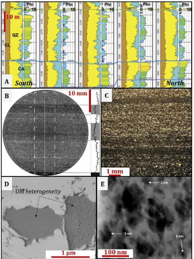
Figure 1. Resolution of various penetration methods, combined with imaging techniques, in common use for porous materials investigation... 31 Figure 2. Geological characteristics of different types of gas reservoir rock (Total.com, 2014). ... 32 Figure 3. Illustration of spatial heterogeneities of shale formation at a multiscale on the example of

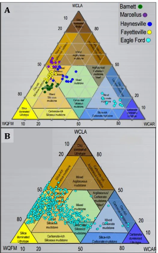
Barnett shale (Fort Worth Basin, Texas, USA). A) North-to-south section through five wells (QZ=Quartz, CL=Clay, CA=Carbonate, Phi= neutron log porosity) (Close et al., 2010). B) µCT image of the core sample (200 keV, voxel size=41.56 μm) (Cronin, 2014). C) Thin-section micrograph (Loucks et al., 2009). D) FIB-SEM (focus ion milling coupled with scaning electron microscopy) image (accelerating voltage=1kV, working distance ~4 mm) (Curtis et al., 2012a). E) ADF STEM (angular dark field scanning transmission electron microscopy) image (Curtis and Ambrose, 2010)... 34 Figure 4. A) Variation of bulk mineral composition for Northern American shales; B) mineral

composition distribution for Barnett shale samples (WCAR = mass fraction of carbonates, WCLA = of clay minerals, WQFM = of quartz/feldspar/micas) (Gamero-Diaz et al., 2012)... 36 Figure 5. A) Van Krevelen diagram of three main types of kerogen (I, II and III), based on the

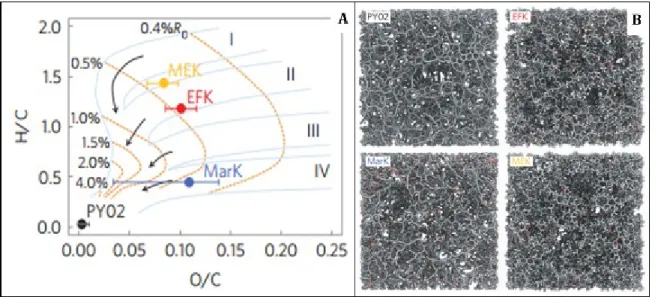
elementary composition: hydrogen-to-carbon (H/C) ratio versus oxygen-to-carbon (O/C) ratio; and theirs evolution curves (after Tissot and Welte, 1984). B) Thermal maturation of kerogen (McCarthy et al., 2011). ... 37 Figure 6. A) Van Krevelen diagram with the representation of the chemical evolution of immature

kerogens of varying sources (Type I, II, III and IV) with increasing levels of maturity: MEK is a type IIS (sulfur reach) kerogen, whereas EFK and MarK are type II marine kerogens, VReq = 0.55, 0.65 and 2.2%, respectively, PYO2 is mineral free shungite; B) molecular models of the four samples under study with density of 1.2 g/cm3_{, carbon, hydrogen and oxygen atoms are} represented in grey, white and red, respectively; the box size is 50 Å in each direction (Bousige et al., 2016). ... 39 Figure 7. Schematic petrophysical model showing volumetric components of gas-shale matrix

(Ambrose et al., 2010). ... 40 Figure 8. Multiscale structure of shale rocks with various heterogeneities, including pores at several

scales, clays, kerogen patches and clastic grains (quartz, calcite, feldspar) embedded into the clay matrix. Relative dimensions of common clay minerals, and schematic view of the microstructure of shales at various scales (Ougier-Simonin et al., 2016)... 42 Figure 9. A) Interfacial contact angle of mercury, measured on various substrates; B) interfacial

contact angle of various substrates on the surface of quartz (Ethington, 1990; information for pyrite is from Bagdigian and Myersont, 1986). ... 45 Figure 10. Uncorrected data from analysis of a glass sample with controlled porosity created of a

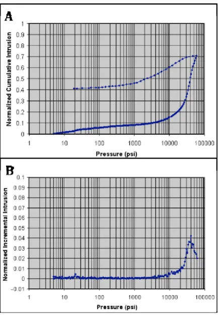
mixture of three pore sizes. The apparent intrusion at size above 10 µm is explained to be due to interparticle filling (Micromeritics, 2012). ... 47 Figure 11. Capillary pressure curve for Barnet shale sample: A) normalized cumulative

(14)

Figure 12. Incremental pore throats sizes distributions obtained for various shales (Clarkson et al., 2013)... 48 Figure 13. Schematic representation of the gas adsorption and desorption processes within cylindrical

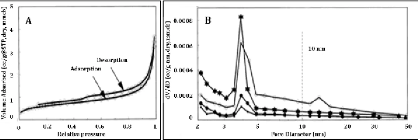
pore. ... 51 Figure 14. A) Nitrogen adsorption and desorption isotherms for coal sample: B) pore size distribution

by BJH transformations on desorption curves (Clarkson and Bustin, 1999a). ... 53 Figure 15. Nitrogen (A) and carbon dioxide (B) isotherms collected for the shale samples (Clarkson et

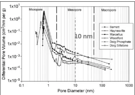
al., 2013). ... 53 Figure 16. Pore size distribution curves for shale samples, defined by differential pore volume using

low-pressure gas (N2 and CO2) adsorption analysis (Chalmers et al., 2012a). ... 54 Figure 17. Nitrogen gas adsorption and desorption isotherms for the samples from lower Silurian black shales (Tian et al., 2013). ... 54 Figure 18. Representative isotherms (A) on natural (in blue) and NaOCl treated (in red) samples and

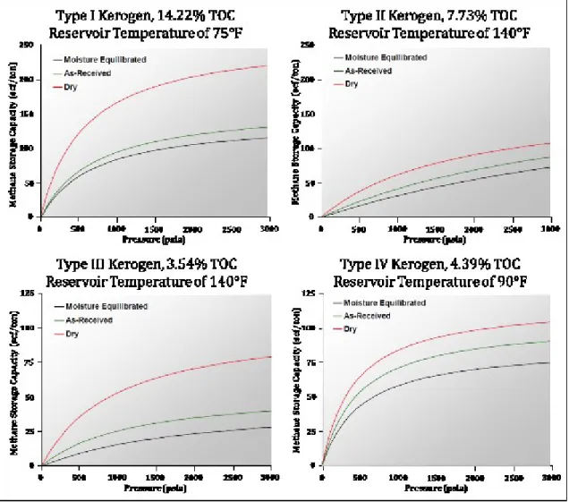
(B) corresponding pore size distribution curves (I+S = illite + smectite clay group in mass%; TOC = Total Organic Carbon in mass%; Eff. = OM removal efficiency in %; HI = Hydrogen Index in mg HC/g TOC) (Kuila et al., 2014). ... 55 Figure 19. Methane adsorption isotherms on powder shale samples of various maturity under different

temperature and humidity conditions (Hartman et al., 2008). ... 57 Figure 20. Pore size distribution of porous rock sample from NMR method (solid line) and from

mercury intrusion (dashed line) (Sørland et al., 2007). ... 60 Figure 21. T2 (relaxation time) – distribution: (1) pure water and (2) pure oil saturated methylated

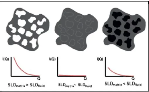
quartz powder; (3) for clean quartz silt; (4) for methylated quartz particle bed (150-180 μm grain size) (Borysenko et al., 2006). ... 60 Figure 22. Fluid or proton typing using T1-T2 map (Fleury and Romero-Sarmiento, 2016)... 62 Figure 23. Qualitative presentation of contrast-matching experiments with fluid saturated porous

systems (Melnichenko et al., 2012). ... 64 Figure 24. SANS measurements result on tight gas samples (Clarkson et al., 2012): A) scattering

profile with background subtracted (solid line represents fit to the power low model applied); B) pore size distribution based on the fitting of polydisperse spherical particles model to the scattering data. Example of SANS measurements result on shale samples (Yang et al., 2017): C) scattering profile with background subtracted; D) pore size distribution based on the fitting of polydisperse spherical particles model to the scattering data. ... 66 Figure 25. Princip of representative elementary area calculation (REA): (A) BSE mosaic is segmented

according to the different gray level and EDX analysis; (B) a stepwise growing grid is placed on the segmented BSE mosaic to perform the box counting method; (C) counting box analysis indicating REA, which is between 100 µm×100 µm and 200 µm×200 µm (Klaver et al., 2012).70 Figure 26. Ion milled surfaces with ion current striations (white arrows) from literature: A) focus ion

beam milling on Haynesville sample, Ga-beam, 2 kV, FE-SEM, area n*100 µm2_{(Chalmers et} al., 2012a); B) broad ion beam milling on Fusinite maceral, Ar-beam, 6 kV, SE, n*100 mm2 (Giffin et al., 2013). ... 71

(15)

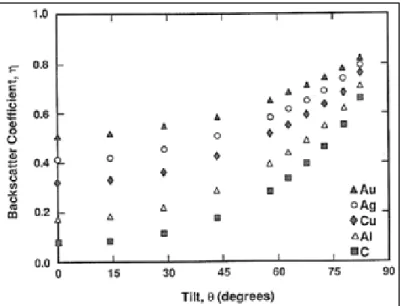
Figure 27. Secondary electron (SE) images for sample after surface impregnation at same scale showing the difference in topography between A) a mechanically polished surface; and B) an Ar-ion beam cut surface (Loucks et al., 2009). ... 72 Figure 28. Backscattered electron coefficient as a function of tilt as calculated for several elements by

Monte Carlo electron simulation (Goldstein et al., 2003). ... 73 Figure 29. Large field and beam drift corrected SEM-BSE mosaics (mineral mapping – left),

performed on manually polished sample and region of interest of the initial BSE images (right) (Fauchille, 2015). ... 73 Figure 30. Rock section (A) and false-colour binary image (B) superposed on the autoradiograph of

the labelled granite sample (porosity level ~1.5%); sample diameter is 32 mm; C) histogram of the spatial porosity distribution ordinate – number of pixels (area units) (Hellmuth et al., 1993). ... 75 Figure 31. Porosity map of the linear cement/clay interface; positions of the porosity sub-areas and

profile measurements are shown; white arrow indicates distance from the interface (Gaboreau et al., 2011). ... 76 Figure 32. Equivalent pore-diameter distributions for Posidonia shale achieved by µCT volumes

segmentation (Kaufhold et al., 2016). ... 78 Figure 33. Linear attenuation coefficient, calculated for various minerals and carbon with increasing

source energy (calculations done with XOP2.4 software; Sanchez del Rio and Dejus, 2011) ... 78 Figure 34. A) Medial ax is for two data sets of Berea sandstone showing different pore network

connectivity estimates depending on the image resolution, i.e., 5.92 μm (left) and 1.85 μm (right) (Noiriel, 2015). B) Mesostructure of Callovo-Oxfordian mudstone visualized (on the left) by synchrotron µCT (voxel 0.34mm; C: carbonates, T: tectosilicates, H: heavy minerals); and corresponding mineral group spatial distribution (on right: red is for carbonates, grey –

tectosilicates, yellow - clay matrix, blue – carbonates) (Robinet et al., 2012). ... 80 Figure 35. Back scattered electron (BSE) scanning electron microscopy (SEM) images acquired with

focused ion beam milling from the gas-mature Haddessen well (Toarcian Posidonia Shale, Germany): areas marked with dashed rectangles in A are magnified in B and C (Han et al., 2017)... 81 Figure 36. Pore size distribution obtained with 3D FIB-SEM: A) pore size distribution for different

samples from German shales, 1kV, voxel size 40x40x25 nm (Kaufhold et al., 2016); B) pore size distribution and volumetric contribution of the pores estimated for the 3D reconstruction of samples taken from Horn River formation (British Columbia, Canada), 1kV, voxel size

2.5x2.5x10 nm (Curtis et al., 2012b). ... 82 Figure 37. 3D FIB volumes of pore thresholding and connected pores segmentation: A) for Horn River

formation (British Columbia, Canada) (1 kV, 2.5x2.5x10 µm) (Curtis et al., 2012b); B) for Haynesville formation (1 kV, voxel size interpolated 7.14 nm) (Dewers et al., 2012). ... 83 Figure 38. A) STEM (HAADF mode) image (~100 nm thick lamella; 200 kV) (Bernard et al., 2010).

B) Segmented 2D TEM image (<100 nm thick lamella; 200 kV, point resolution 0.14 nm, field of view 2µm) (Gaboreau et al., 2016). ... 85 Figure 39. A) Transmission electron microscopy image (high-angle annular dark-field, Z-contrast

(16)

appears dark, and silicates and carbonates appear gray; (B) Energy-dispersive x-ray spectroscopy elemental maps: carbon (C), silicon (Si), calcium (Ca), and aluminum (Al). Authigenic calcium carbonates (Cc) and quartz (Qz) cements are identified (Han et al., 2017). ... 85 Figure 40. Monte Carlo electron trajectory simulations of the interaction volume in iron as a function

of beam energy (Goldstein et al., 2003). ... 87 Figure 41. Histogram showing porosity measured by group of researches using subjective methods

alone to manually threshold (Tovey and Hounslow, 1995). ... 88 Figure 42. Pore pace characterization of synthetic compacted illite sample: A1) SE image thresholded

by the Otsu method; A2) EsB image representing the advanced approach of the segmentation of the smallest pores (the red outlines represent the borders of the pores recognized and

thresholding); B) region of interest illustrating the pores segmented from Otsu thresholding (light blue) and from the developed method (yellow); C) intercomparison of pore size distribution achieved by various techniques (Gaboreau et al., 2016). ... 89 Figure 43. Scales and techniques used in correlative multi-scale imaging data of shales (Ma et al.,

2017a). ... 96 Figure 44. FIB-SEM images of some American shales samples (Curtis and Ambrose, 2010). ... 97 Figure 45. Localized 2D FIB-SEM imaging (at 1kV) of OM within the shale sample: A), B) organic

matter of different maturity (Curtis et al., 2012a); C) porous kerogen (Chalmers et al., 2012a); D) heterogeneous organic matter of the same maturity (Curtis et al., 2012a). ... 98 Figure 46. A) Relationship between micropores volume and TOC for Devonian-Mississippian shale

(r²= 0.4, not shown); B) variation in micropores volume with TOC for Jurassic shales (Ross and Marc Bustin, 2009). ... 99 Figure 47. Crossplots of average pore diameter versus average pore volume, obtained by N2 adsorption

(ADI - Adsorption-Desorption Isotherm) for (A) native samples, and (B) cleaned samples (treated with 4:1 mixture of toluene and methanol at 110°C for 24h) from various maturity windows (Ojha et al., 2017). ... 100 Figure 48. Relationship between total porosity volume (achieved by gas adsorption isotherms) and

TOC (data combined from Clarkson et al., 2013; Chalmers et al., 2012a; Ross and Marc Bustin, 2009; Mastalerz et al., 2013; Ma et al., 2015; Kelly et al., 2015; Wust et al., 2014; Han et al., 2017): A) data with thermal maturity based on vitrinite reflectance measurements (R0%); B) data with thermal maturity based on Tmax measurements. ... 101 Figure 49. A) Simplified diagram displaying common diagenetic pathways of coccolithic Eagle Ford

sediments, emphasizing processes with the greatest effects on porosity (see the description in the text) (Pommer and Milliken, 2015). B) Evolution of Minerals and Pore Types in the Eagle Ford Marine Mudrocks (Ko et al., 2017). ... 102 Figure 50. Plot comparing visible total porosity from point-count methods with helium porosity from

crushed-rock Gas Research Institute analysis (avg = average) (Ko et al., 2017). ... 103 Figure 51. A) Cumulative Mercury intrusion and extrusion curves, as a function of pore-throat size;

full symbols indicating uncorrected data and transparent symbols, data corrected for surface roughness effects. Total BIB-SEM visible porosities at practical pore detection resolutions (PPRs) are indicated by squared symbols (Hemes et al., 2014); B) the intercomparison of PSD obtained by MIP and FIB-SEM (1 kV, interpolated voxel size is 7.14 nm) (Dewers et al., 2012);

(17)

C) Sorted cumulative volumetric distributions (SVPD) based on mercury intrusion porosimetry (MIP) and focused ion beam (FIB) pore network models (green and blue lines are for MIP, red – for FIB, example for upper Kirtland data) (Heath et al., 2011). ... 104 Figure 52. The comparison of the results of pore network characterization of Posidonia shale samples.

A) µCT images segmentation and pore size destribution (180 kV, 15W). B) FIB-SEM

segmantation and fpores feret diameteres destribution. C) results of gas adsorption (N2 and CO2) and mercury intrusion measurements (Kaufhold et al., 2016). ... 107 Figure 53. The intercomparison of porosity measurements for some shales (Chalmers et al., 2012a;

Clarkson et al., 2013; Curtis et al., 2012b; Milliken et al., 2013). ... 109 Figure 54. Stratigraphic subdivision of the Late Jurassic to Early Cretaceous successions in the

Neuquén Basin in the subsurface areas within along the Andean foothill (left) and the Neuquén Embayment (right) (Zeller, 2013). ... 113 Figure 55. A schematic distribution of various hydrocarbons areas within the Vaca Muerta formation

(modified from Schmidt et al., 2014). The stars indicate the approximate locations of the

samples, selected for the present study. ... 114 Figure 56. Vaca Muerta kerogen types plotted on a modified van Krevelen diagram (stippled)

(Magoon and Dow, 1994). ... 114 Figure 57. Well log data, given for the wells of interest (the locations of the seven core samples of this

study are indicated with stars)... 115 Figure 58. The well log data corresponding to the selected cores... 118 Figure 59. Damaged core (core F, oil window): A) photo of the core “as received”; B) central slice of

the µtomography volume, acquired on the core (note the cracks at the mm scale all over the core). ... 119 Figure 60. Methods of pore network characterization and their resolutions: A) applied on shale

samples in literature; B) applied in the present research. ... 121 Figure 61. µTomography 3D visualization and subsamples localization (core sample B, condensate

zone): A) virtually cut core (IS – block for impregnation and imaging techniques application, the green line corersponds to the position of the surace polished; BS – block for bulk porosity measurements; PS – blocks for measurements on powder; NMR – blocks for nuclear magnetic resonance spectroscopy); B) virtual cut and image analyses, evaluating the core vertical heterogeneities (central slice, Z-projection of maximum values thorough the block and vertical LAC profile with 300 pix width). ... 123 Figure 62. Visualization of BS block from the sample core H (dry gas window): A) 3D view with

cracks (in green) and “heavy” grains (in yellow) segmented and corresponding z-projection of average values; B) 3D view with carbonates (in blue) and “heavy” grains (in yellow) segmented and corresponding z-projection of maximum values (note that some of the pixels, located around heavy grains, are in the same range of intensity as carbonates, due to X-Ray scattering artifacts). ... 124 Figure 63. Left: procedures used for preparing grain density measurements by He-pycnometry. Right:

localization of sub-blocks used for grain density measurements by He-pycnometry (illustrated on 3D view of virtually subsampled core D, condensate zone)... 127

(18)

Figure 64. Left: virtually sub-sampled BS-block (MIP – mercury intrusion porosimetry, Ads –

nitrogen adsorption). Rigth: a scanned individual sub-sample block. ... 129 Figure 65. A) Impregnation cell. B) Scheme of the sample “sandwich” preparation for the

impregnation (after Prêt, 2003). ... 130 Figure 66. A) Polishing set Tegramine-30 (Struers); B) sample holder, adapted for large samples

surfaces preparation. ... 131 Figure 67. A) Microscope Leica DCM8 at confocal scanning mode (photo from

http://www.leica-microsystems.com); B) general principle of confocal microscopy (after Minsky, 1988)... 132 Figure 68. Workflow of Image treatment by Leica-Map ©. ... 133 Figure 69. Example of analyses of images recorded at x100 magnification with confocal microscope.

... 134 Figure 70. CFM images (calibration bar: ±2µm, scale bar: 200µm) of the central part of impregnated

sample C (condensate zone) at different polishing steps with the indication of surface roughness: A) in the end of polishing with 5 µm SiC foil disc; B) in the end of polishing with 1µm

suspension; C) final surface in the end of 1/4 µm step; D) BSE-SEM image on the center of the same sample prepared for the autoradiography (FEG-SEM Zeiss Ultra 55, accelerating voltage - 5 kV, working distance - 10.3 mm). ... 135 Figure 71. A) Scheme of the procedure of autoradiography exposition (modified from Prêt, 2003); B)

an example of the scanned film, after development, with samples (dark grey rectangles, white rings correspond to the non-porous resin, surrounding the sample) and standards of pure 14 C-PMMA with known activity (in orange rectangles). ... 136 Figure 72. Calibration curve, obtained by the optical density of the standard with known activity,

collected for the VM samples exposition, plotted together with pixl value frequence histograms collected over the ful autoradiograph surface. ... 137 Figure 73. A scheme for the correlation of autoradiography porosity maps with other techniques:

layers of interest and projections of blocks, where bulk measurements were performed, can be found on the autoradiography surface (green line) to extract the connected porosity value of corresponding area (𝜑𝐴𝑢𝑡𝑜𝐶𝑜𝑛_𝐿 and 𝜑𝐴𝑢𝑡𝑜𝐶𝑜𝑛_𝐵, respectively). ... 139 Figure 74. The trend graph, tracking the pressure equilibrium in the system over nitrogen adsorption

measurements. ... 140 Figure 75. A) Spatial distribution of the backscattered electrons emission within the homogeneous

material (after Prêt, 2003). B) Depth (PBSE) and the diameter (DBSE) of the zone of backscattered electrons emmision as a function of incident beam energy (E0) for mineral and organic phases (assuming the beam normal to the sample surface, tilt = 0°), calculated by Kanaya – Okayama equation (Kanaya and Okayama, 1972): blue lines are for the range of the dimensions for the phases in this stydy; green sqeare is for the pixel size, selected for the BSE-SEM mosaics. ... 144 Figure 76. The ATLAS5© window screenshot, during the three points correlation process of

autoradiograph and SEM FOV. ... 145 Figure 77. Mean filter application on the autoradiography images (display grey level range is 50-200,

ROI to display is 400x400 pixels, histograms were collected on ROI of 2412x2412 pixels, 1 pixel = 10.65 µm). ... 149

(19)

Figure 78. Median filter application on the autoradiography images (display grey level range is 50-200, ROI to display is 400x400 pixels, histograms were collected on ROI of 2412x2412 pixels, 1 pixel =10.65 µm). ... 150 Figure 79. Gaussian filter application on the autoradiography images (display grey level range is

50-200, ROI to display is 400x400 pixels, histograms were collected on ROI of 2412x2412 pixels, 1 pixel =10.65 µm). ... 151 Figure 80. NLM filter application on the autoradiography images (display grey level range is 50-200,

ROI to display is 400x400 pixels, histograms were collected on ROI of 2412x2412 pixels, 1 pixel =10.65 µm). ... 152 Figure 81. Porosity values recalculated from published literature data sets (e.g., gas adsorbed and

intruded mercury volumes), obtained using various methods on several unconventional shale formations: He – helium pycnometry, MIP – mercury intrusion porosimetry, SANS – small angle neutron scattering, SEM – scanning electron microscopy, micropores – porosity measured by CO2 adsorption, mesopores & macropores – porosity measured by nitrogen adsorption and mercury intrusion (the displayed data are not exhaustive but representative of most litterature data). ... 157 Figure 82. a) 3D µtomography exploded view of sample B (condensate zone) showing the localization

of the different sub-samples within the full core: IS – block for impregnation and imaging techniques; BS – block for bulk porosity measurements; PS1&PS2 – blocks for powder analyses (quantitative mineralogy, He-pycnometry, TGA-MS); NMR1&NMR2 – blocks for nuclear magnetic resonance spectroscopy; b) 2D slice from 3D volume and Z projection of maximum pixel values displaying the distribution of the heavy grains (MIP – blocks for mercury intrusion porisimetry, Ads – blocks for gas adsorption); c) 3D view of the BS block showing the virtual cut of the samples used for bulk porosity measurements; d) 3D view of one of the sub-sampled blocks with improved resolution; e) a scheme for the correlation of autoradiography porosity maps with other techniques: layers of interest and projections of blocks where bulk measurements were performed can be found on the autoradiography surface to extract the

connected porosity value of corresponding areas (𝜑𝐴𝑢𝑡𝑜𝐶𝑜𝑛_𝐿, 𝜑𝐴𝑢𝑡𝑜𝐶𝑜𝑛_𝐵, respectively). 160 Figure 83. Results of the thermal analysis: a) first derivative of the mass loss for samples from

different hydrocarbon production zones; b) mass spectra of some compounds detected under thermal stress for sample F. ... 164 Figure 84. Porosity maps obtained by autoradiography for three core samples with, on their right, a

vertical porosity profile through the center of the image (yellow line) obtained by

autoradiography (in light gray, profile with 1-pixel width and in black – profile with 500-pixel width) and a LAC vertical profile through the center of the corresponding slice (yellow line) from µtomography 3D volume (in gray – with 1-pixel width and in black – profile with 300-pixel width); Quantitative mineralogical compositions are indicated for the layers of interest (purple – clay minerals, green – tectosilicates; blue – carbonates, orange – pyrite, red – accessory minerals, black – IOM). ... 166 Figure 85. Pixel frequency histograms over the full autoradiography porosity maps. ... 167 Figure 86. Autoradiography porosity map and frequency histograms of the IS block of sample B

(20)

autoradiography image are plotted on the left (in light gray - profile with 1-pixel width and in black – profile with 500-pixel width); quantitative mineralogical compositions are indicated for the layers of interest (purple – clay minerals, green – tectosilicates; blue – carbonates, orange – pyrite, red – accessory minerals, black – IOM); the corresponding area of the blue rectangle, extracted from the µtomography slice, is shown on the bottom right corner. ... 169 Figure 87. a) Connected porosity values measured by NMR using Equation 30 versus the total

porosity, according to the Equation 38, estimated on the same blocks; b) porosity values obtained by MIP (closed symbols, φMIP) and gas adsorption (open symbols, φAds), measured on the

localized sub-blocks; triangles are for gas zone samples, squares - for condensate zone, circles - for oil zone. ... 170 Figure 88. a) Cumulative intrusion and extrusion curves from different hydrocarbon maturity zones

and porosity values measured by MIP (open symbols) and total porosity measured on NMR blocks (closed symbols), given for the samples from the same layers of interest; b) Normalized MIP cumulative intrusion curves (normalized according to the total porosity on NMR blocks) and incremental throat size distributions. Black dotted lines are for the different techniques’ resolutions; blue lines and symbols are for the oil zone sample; red lines and symbols are for the condensate zone sample; and green lines and symbols are for the gas zone sample. ... 171 Figure 89. a) Nitrogen gas adsorption/desorption curves, obtained for the block (red symbols) and

powder (gray symbols) from the core sample C (condensate zone); b) BJH cumulative distributions calculated for the block and powder (open symbols are for the pore throat sizes distribution, closed symbols – for the pore body sizes distribution). The reference total porosity value, obtained on NMR blocks for the corresponding layer, is marked with a diamond symbol. ... 173 Figure 90. Nitrogen adsorption/desorption isotherms obtained on the different localized sub-samples:

for oil (circles), condensate (squares) and dry gas (triangles) zones. ... 174 Figure 91. Cumulative pore size distribution with indication of total porosity measured by laser on

NMR blocks (diamond symbol) for the corresponding layer of interest: a) pore body diameter distribution, calculated from the nitrogen adsorption curves (triangles are for gas zone samples, squares for condensate zone, circles for oil zone); b) pore throat diameter distribution calculated from the nitrogen desorption curves (open symbols; data for sample F are corrected by

combination with results of MIP porosity >640 nm) and from MIP intrusion curves (lines). .... 175 Figure 92. a) Quantitative porosity measurements from the autoradiography surface on the localized

layers of interest (closed symbols) and on projections of blocks on the autoradiography surface (open symbols), where other bulk techniques were applied: triangles are for gas zone samples, squares - for condensate zone, circles - for oil zone; b) total porosity on MIP blocks and total µtomography porosity on the same blocks, calculated from the measured dry bulk densities and the grain density measured on NMR blocks: stars. ... 178 Figure 93. Porosity balances based on the combination of bulk measurements: 𝜑𝑁𝑀𝑅𝑇– total porosity on NMR blocks, 𝜑𝑀𝐼𝑃𝑇–total porosity on MIP blocks, 𝜑𝐴𝑢𝑡𝑜𝐶𝑜𝑛– autoradiography connected porosity for localized layers, 𝜑𝑀𝐼𝑃 > 640𝑛𝑚– results of the porosity, corresponding to the MIP volumes intruded into the pores with pore throat >640 nm, 𝜑𝐴𝑑𝑠𝑚𝑒𝑠𝑜 − 𝑚𝑎𝑐𝑟𝑜 – measured adsorption porosity > 2 µm, 𝜑𝐴𝑑𝑠µ- microporosity < 2 µm, revealed by gas adsorption. ... 180

(21)

Figure 94. A) The two concepts of crystal structure of mixed-layer minerals: McEwan crystallite (top) and fundamental particle (bottom) (Meunier, 2005). B) Organisation of the mixed-layered minerals structure with the illite (A) and smectite (B) layers (Brigatti et al., 2013). ... 197 Figure 95 Position of the VM samples on the shales samples ternary plot classification: A) proposed

by Passey et al. (2010); B) proposed by Gamero-Diaz et al. (2012). ... 199 Figure 96. dTG curves, recorded for dry gas sample (powder from the core H) in argon (thin line) and

air (thick line) atmospheres with a 1°C/min heating ramp. ... 200 Figure 97. Weight loss (doted lines) and dTG (solid lines) curves recorded for samples from zones

with various hydrocarbons types (blue lines are for oil window, sample F; red – for condensate zone, sample C; green – for gas window, sample H); with a heating ramp of 5 °C/min in an argon atmosphere. ... 201 Figure 98. Results of TGA-MS analysis for samples from zones with various hydrocarbons types

(5°C/min, argon atmosphere): A) derivative weight loss curves; B) spectra of mass 18 (H2O); C) spectra of mass 44 (CO2); D) spectra of mass 64 (SO2/S2)... 206 Figure 99. Result of TGA-MS analysis for samples from zones with various hydrocarbons types

(5°C/min, argon atmosphere): A) derivative weight loss curves; B) spectra of mass 41 (C3H5); C) spectra of masses 50 (C4H2) and 57 (C4H9); these compounds have been detected only for

samples F and H (no data for sample C is present); D) spectra of mass 76 (C6H4). ... 207 Figure 100. Connected porosity values, measured by NMR using Equation 30 and Equation 31, versus

the total porosity, measured on the same blocks (triangles are for gas zone samples, squares – for condensate zone, and circles – for oil zone). ... 210 Figure 101. Mercury intrusion porosimetry results for zones of various hydrocarbons production; on

the right: non-normalized cumulative intrusion and extrusion curves and porosity values measured by MIP (closed symbols, 𝜑𝑀𝐼𝑃) and total porosity measured on NMR blocks (open symbols, 𝜑𝑁𝑀𝑅𝑇), given for the samples from the same layers of interest; on the left:

normalized MIP cumulative intrusion curves (normalized according to the total porosity measured on NMR blocks) and incremental throat size distributions: A) for oil window; B) for condensate zone; C) for dry gas window. ... 212 Figure 102. Gas adsorption on blocks of the different localized sub-samples: for oil (circles),

condensate (squares) and dry gas (triangles) zones: A) nitrogen adsorption/desorption isotherms; B) cumulative pore body diameter distributions, calculated from the adsorption curves; C) cumulative pore throat diameter distribution calculated from the desorption curves; with indication of total porosity measured by laser on NMR blocks (diamond symbol) for the

corresponding layer of interest. ... 214 Figure 103. Correlation of the connected porosity (measured by NMR and autoradiography) with total

porosity (measured by laser): triangles are for gas zone samples, squares for condensate zone, and circles for oil zone. ... 216 Figure 104. Pixel value frequency histograms over the full surfaces and porosity maps obtained, by

autoradiography for core samples with, on their right, a vertical porosity profile through the center of the image (green line; in light gray – profile with 1-pixel width, and in black – profile with 500-pixel width); maps are ranged in 0-30% porosity values; LUT = Phase. ... 217

(22)

Figure 105. A) Pore balances obtained by combination of various techniques, applied on the sub-block from layer 2, core F (oil window); B) the 3D view of virtual cut of sub-block for MIP

measurements; C) segmented cracks within the sub-block for MIP measurements. ... 219 Figure 106. Core sample E (oil window): A) MIP intrusion and extrusion curves; open diamond

symbol is for the MIP intrusion porosity (𝜑𝑀𝐼𝑃), close diamond – for total porosity on NMR blocks (𝜑𝑁𝑀𝑅𝑇); B) normalized MIP cumulative intrusion curve and incremental throat size distribution; C) µtomography central slice of BS block with the localization of sub-blocks positions and obtained porosity values; mineral composition is indicated for the layers of

interest; on the right: LAC profile plotted through the center of the core (yellow line). ... 223 Figure 107. Core sample F (oil window): A) MIP intrusion and extrusion curves; BJH pore throat

distribution from N2 desorption curve; open diamond symbol is for the MIP intrusion porosity (𝜑𝑀𝐼𝑃), close diamond – for total porosity on NMR blocks (𝜑𝑁𝑀𝑅𝑇); B) BJH pore body size distribution from N2 adsorption curve; C) µtomography central slice of BS block with the localization of the sub-blocks positions (colors are corresponding to the color of the curve from the PSD) and obtained porosity values; mineral composition is indicated for the layers of

interest; on the right: LAC profile plotted through the center of the core (yellow line); D) porosity map obtained by autoradiography with a vertical porosity profile through the center of the image (green line). ... 224 Figure 108. Core sample B (condensate zone): A) MIP intrusion and extrusion curves; BJH pore

throat distribution from N2 desorption curve; open diamond symbol is for the MIP intrusion porosity (𝜑𝑀𝐼𝑃), close diamond – for total porosity on NMR blocks (𝜑𝑁𝑀𝑅𝑇); B) BJH pore body size distribution from N2 adsorption curve; C) µtomography central slice of BS block with the localization of the sub-blocks positions (colors are corresponding to the color of the curve from the PSD) and obtained porosity values; mineral composition is indicated for the layers of interest; on the right: LAC profile plotted through the center of the core (yellow line); D) porosity map obtained by autoradiography with a vertical porosity profile through the center of the image (green line). ... 225 Figure 109. Core sample C (condensate zone): A) MIP intrusion and extrusion curves; BJH pore

throat distribution from N2 desorption curve; open diamond symbol is for the MIP intrusion porosity (𝜑𝑀𝐼𝑃), close diamond – for total porosity on NMR blocks (𝜑𝑁𝑀𝑅𝑇); B) BJH pore body size distribution from N2 adsorption curve; C) µtomography central slice of BS block with the localization of the sub-blocks positions (colors are corresponding to the color of the curve from the PSD) and obtained porosity values; mineral composition is indicated for the layers of interest; on the right: LAC profile plotted through the center of the core (yellow line); D) porosity map obtained by autoradiography with a vertical porosity profile through the center of the image (green line). ... 226 Figure 110. Core sample D (condensate zone): A) MIP intrusion and extrusion curves; open diamond

symbol is for the MIP intrusion porosity (𝜑𝑀𝐼𝑃), close diamond – for total porosity on NMR blocks (𝜑𝑁𝑀𝑅𝑇); B) normalized MIP cumulative intrusion curve and incremental throat size distribution; C) µtomography central slice of BS block with the localization of the sub-blocks positions (colors are corresponding to the color of the curve from the PSD) and obtained porosity values; mineral composition is indicated for the layers of interest; on the right: LAC profile

(23)

plotted through the center of the core (yellow line); D) porosity map obtained by autoradiography with a vertical porosity profile through the center of the image (green line)... 227 Figure 111. Core sample H (gas window): A) MIP intrusion and extrusion curves; BJH pore throat

distribution from N2 desorption curve; open diamond symbol is for the MIP intrusion porosity (𝜑𝑀𝐼𝑃), close diamond – for total porosity on NMR blocks (𝜑𝑁𝑀𝑅𝑇); B) BJH pore body size distribution from N2 adsorption curve; C) µtomography central slice of BS block with the localization of the sub-blocks positions (colors are corresponding to the color of the curve from the PSD, test on orange block was failed) and obtained porosity values; mineral composition is indicated for the layers of interest; on the right: LAC profile plotted through the center of the core (yellow line); D) porosity map obtained by autoradiography with a vertical porosity profile through the center of the image (green line). ... 228 Figure 112. Core sample I (gas window): A) MIP intrusion and extrusion curves; open diamond

symbol is for the MIP intrusion porosity (𝜑𝑀𝐼𝑃), close diamond – for total porosity on NMR blocks (𝜑𝑁𝑀𝑅𝑇); B) normalized MIP cumulative intrusion curve and incremental throat size distribution; C) µtomography central slice of BS block with the localization of the sub-blocks positions (colors are corresponding to the color of the curve from the PSD) and obtained porosity values; mineral composition is indicated for the layers of interest; on the right: LAC profile plotted through the center of the core (yellow line); D) porosity map obtained by autoradiography with a vertical porosity profile through the center of the image (green line)... 229 Figure 113. A scheme of correlative mineralogical and porosity quantification throught the

comparison of autoradiography and SEM mosaic results. ... 235 Figure 114. Correlation of total porosity measured on NMR blocks with mineral composition for the

same layers of interes, measured by XRD-XRF method: A) non-porous matter volumetric contents (*sum of quartz, albite, carbonates, pyrite and accessory minerals); B) porous matter (clay minerals and IOM) volumetric contents. Circles are for samples from oil window; squares – for condensate zone; and triangles – for the dry gas window. ... 236 Figure 115. Porosity map obtained by autoradiography with positions of the BSE-SEM mosaic (blue

rectangles); on the right, a vertical porosity profile through the center of the image (green line) and the corresponding BSE-SEM mosaic overview; mineral composition is indicated for the layers of interest, on the left and black rectangles correspond to the projection of blocks used for bulk porosity measurements. ... 238 Figure 116. One individual initial tile acquired from a full mosaic (left) and the mineral map

segmented from the same area of the recalculated full mosaic (right). ... 239 Figure 117. A) The overview of the acquired mosaic (C_IS, core C, condensate) with the location of

ROI (orange and red squares) observed at full magnification (C and D); B) horizontal profile at mid height of the mosaic (orange line, 100 pixels width); D) grey level frequency histograms of orange and red ROI. ... 240 Figure 118. Effect of varying the z position of the sample surface on solid angle of detection of BSE

and simultaneous defocusing. ... 241 Figure 119. Illustration of the treatment done to normalize the histograms of the set of tiles of the

mosaic of sample F. Left: Scatterplot of the set of initial grey level histogram, one line corresponds to one histogram viewed from the top and with a color encoding of the pixel

(24)

frequency. Centre : Scatterplot of the normalized histograms. Right: Initial and normalized histograms of the tiles of columns 6 and 30 of the second row of the mosaic. ... 242 Figure 120. Large BSE mosaic of sample F (top) and the resulting mineral map (bottom). The ROI

black, yellow and blue (centre) correspond to a contineous zooming at one location of the map. Carbonates in red , tectosilicates in blue and purple, solid organic matter in orange tones , resin in black, heavy minerals in yellow and clay matrix in green. ... 244 Figure 121. Mineral map (top) and the associated mapping of the volumetric contents of the main

phases by a sliding windows approach. ... 245 Figure 122. Horizontal profiles of volumic phase contents along the large field mineral map. On top,

porosity evolution according to the SEM mosaic segmentation (macropore evolution in black) and by autoradiography (macropore, mesopore and micropore) and the two others graphs represent the evolution of the segmented phases obtained from the SEM mosaic mineralogical map. ... 246 Figure 123. Horizontal profiles of weight phase concentrations and SEM/autoradiograph porosities

along the large field mineral map. ... 247 Figure 124. Porosity balances based on the combination of bulk measurements and imaging

techniques: 𝜑𝑁𝑀𝑅𝑇– total porosity on NMR blocks, 𝜑𝑀𝐼𝑃𝑇–total porosity on MIP blocks, 𝜑𝐴𝑢𝑡𝑜𝐶𝑜𝑛– autoradiography connected porosity for localized layers, 𝜑𝑀𝐼𝑃 > 640𝑛𝑚– results of the porosity, corresponding to the MIP volumes intruded into the pores with pore throat >640 nm, 𝜑𝐴𝑑𝑠𝑚𝑒𝑠𝑜 − 𝑚𝑎𝑐𝑟𝑜 – measured adsorption porosity > 2 µm, 𝜑𝐴𝑑𝑠µ- microporosity < 2 µm, revealed by gas adsorption, 𝜑𝑆𝐸𝑀 > 640𝑛𝑚 – porosity obtained from the segmented SEM mosaics. ... 248 Figure 125. Autoradiograph porosity frequency histo grams of F-IS sub-sample surface initially

obtained for an exposure time of 149h and latter for 295h, after repolishing for SEM imaging techniques application. ... 249 Figure 126. The correlation of large field autoradiography porosity map with the mineral map,

calculated from BSE-SEM mosaic. Top: porosity map; center: correlative plot of mean porosity vs the sum of tectosilicates and carbonates (vol%), sliding windows of 200 µm size; bottom: BSE-SEM mineral map ... 250 Figure 127. Correlation of connected porosity obtained from autoradiography with mineral phases

distribution, obtained from BSE-SEM mosaics. Left: porous matter (clay minerals and IOM) volumetric contents; right: non-porous matter (tectosilicates and carbonates) volumetric contents. Circles are for samples from oil window; squares – for condensate zone; and triangles – for the dry gas window. ... 251

(25)

List of tables

Table 1. Summary of imbibed volumes, measured from weight changes after the second imbibition sequence. Reported volumes are normalized to the bulk volumes of the samples (cm3_/cm3₎ (Odusina et al., 2011)... 40 Table 2. Average diameters of different gases (after Vermesse et al., 1996; data for CO2 is from

D'Alessandro et al., 2010). ... 49 Table 3. Proportion of pores <5 nm estimated as the sum of micropore (<2 nm) volume (derived from

N2 adsorption isotherm applying t-plot method) and total pore volume between 2 and 5 nm pores size (estimated from BJH inversion with Harkins-Jura thickness equation) (see details in Kuila et al., 2014). ... 56 Table 4. A) Comparison of SLD values for the shale samples (Clarkson et al., 2012). B) SLD values

for some compounds expected in shale sample (calculated by “NICT neutron activation and scattering calculator” for neutron source λ=4.8 Å; NIST, 2015). ... 65 Table 5. Dehydration temperatures for different clay minerals (Grim and Bradley, 1948). ... 67 Table 6. Comparison of the parameters of various monomers with water. ... 75 Table 7. Acquisition and data treatment parameters selected for different imaging techniques and

applied for the shale samples characterization. ... 90 Table 8. The results of the characterization of the pore space by a combination of methods (Kaufhold

et al., 2016). ... 106 Table 9. Mineral compositions and physical parameters estimated from log data by a calibrated

MULTIMIN© approach for the selected samples from three different exploration wells in zones of various hydrocarbon maturities (Vreq - maximum thermal maturity measured on bitumen, LAC – linear attenuation coefficient, DTSM – shear slowness, DTCO – compressional slowness, PhiT – total porosity, PhiE – effective porosity). ... 120 Table 10. Time required for the N2 adsorption/desorption acquisition on blocks. ... 141 Table 11. A) Parameters selected for the mosaics acquisition. B) Dimensions and acquisition time for

the acquired mosaics (8-bit images). ... 145 Table 12. Result of the filters, selected for image denoizing ... 148 Table 13. Mineral compositions and physical parameters estimated from log data by a calibrated

MULTIMIN © approach for the selected samples from three different exploration wells in zones of various hydrocarbon maturities (Vreq - maximum thermal maturity measured on bitumen, LAC – linear attenuation coefficient, DTSM – shear slowness, DTCO – compressional slowness, PhiT – total porosity, PhiE – effective porosity). ... 185 Table 14. Quantitative mineraligal compositions obtained using the MinEval method of Total on the

localized layers of interest within the selected cores (*sum of barite, anatase and apatite). Errors are in the order of +/- X0.35_{mass% at 95% confidence (for example 30.0 +/- 3.3 mass%). ... 186} Table 15. Total porosity values calculated or measured on comparable blocks by different techniques

(*for total porosity values the method for bulk volume measurement is indicated; grain density was obtained by He-pycnometry on plugs; NMR – nuclear magnetic resonance spectroscopy; MIP – mercury intrusion porosimetry). ... 187

(26)

Table 16. Quantitative mineralogic compositions obtained with the MinEval method of Total on the localized layers of interest within the selected cores (*sum of barite, anatase and apatite). Errors are in the order of ± X0.35_{mass% at 95% confidence (for example, 30.0 ± 3.3 mass%). ... 196} Table 17. CEC measurements and XRD mineral composition results of the fraction <5µm, on the

localized layers of interest within the selected cores (PT – possible trace; *calculations done assuming theoretical CEC of pure illite of 25 meq/100g and CEC of pure montmorillonite of 80 meq/100g, Meunier, 2005). ... 198 Table 18. Results of grain and bulk densities measurements by various techniques... 209 Table 19. Penetration methods limitations and assumptions used in literature for shale samples

characterization. ... 233 Table 20. Imaging techniques and achieved resolutions. ... 234 Table 21. Symbols used in the manuscript. ... 257 Table 22. Abbreviations used in the manuscript. ... 261 Table 23. Conversion of parameters used in the literature and in the manuscript to the SI units (Taylor

and Thompson, 2008). ... 263

(27)

Introduction

During the last decades, since 90’s, the interest to the unconventional hydrocarbons sources has been significantly increased due to fast development of the industry, which requires more and more energy every year, and, at the same time, the depletion of the conventional sources. The development of alternative sources of energy (such as Sun, wind, alternative fuels, etc.) is still not covering the needs of the modern economic, while high productive atomic energy branch is remaining at a constant level with high risks during the nuclear plants exploitation.

Meanwhile, the exploitation of unconventional forms of gas and oil and the rapid shift from the dominance of traditional producers to plentiful domestic resources in many countries represents the dawn of a new era in global energy. There is the potential for job creation, business revitalization, the creation of markets for new by-products, greater energy independence, and newfound wealth for land owners, municipalities, and governments that hold subsurface mineral rights (Arthur and Cole, 2014).

In 2013, the U.S. Energy Information Administration estimated, that 4644 trillion cubic feet of gas-in-place could exist in potential shale gas formations in the United States (EIA, 2013). Shales, which are the organic rich sedimentary rocks, thus play an increasingly significant role in countries like U.S. for the energy supply. However, shale formation is still hard to evaluate using routine core analysis or petrophysical techniques, because of the compositional heterogeneity, pore structure complexity, and fine-grained nature of the rock. In the case of organic shales, large variations in formation properties and characteristics can exist both, laterally and vertically.

Understanding the geological and geochemical nature of gas shale formations and improving their productivity, thus, have been “at the heart of millions of dollars’ worth” of research since the 1970’s (Bernard et al., 2010). Indeed, the specific geological characteristics and structural features of unconventional formations create some potential risk due to fracturing processes, which, at the same time, may cause the uncontrolled migration of liquid hydrocarbons.

One of the main problem is water viability, as exploration requires big volumes of water, and the water contamination, which may impact to ground and surface water quality, public and private water supplies. Like that, the reduction of the local water resources quality has been detected in the areas of the long-term developing shale deposits in the Northern America (Vidic et al., 2013).

Another negative effect of uncontrolled gas or/and oil migration, which leads to the hazard impact on human infrastructure and environment by itself, is a release of naturally occurring radioactive materials and trace elements from the formation. Finally, the

(28)

atmospheric impacts of hydrocarbons extraction and utilization must be kept in mind to provide effective regulation and execution of such processes.

In general, the following targets of the investigations dealing with shale pore space can be underlined:

- disclosing the areas of hydrocarbons storage;

- describing the pathways of gas/oil migration from matrix;

- evaluation of parameters, controlling its microstructure of formation; - improving the extraction techniques and productivity;

- preventing the negative effects from extracting processes;

- prediction and modelling of the reservoir properties (gas/oil storage capacity, permeability, mechanical behavior etc.).

To prevent the negative effects on the exploitation of these unconventional deposits, it is important to evaluate the potential behavior and the possibility for their safe extraction. The detailed investigation of shale rocks microstructure allows to disclose the areas of hydrocarbons storage and to evaluate the storage capacity of the formation, the mechanical behavior of the geological formation under hydraulic fracturing stress, and possible hydrocarbons migration pathways within the whole reservoir. Some works on different shales have been already presented in the literature being dedicated to the estimation of the parameters, which control their microstructure formation. The characterization of the pore sizes distribution, pores connectivity and pores morphology can improve the knowledge about the shale microstructure. These characteristics are crucial for the correct description of unconventional reservoirs and required for the preventing negative effects from extracting processes and for enhancement of the extraction techniques by themselves, that can lead to the significant increase of the productivity.

Since the 80’s, all the studies, which are dedicated to the characterization of gas shale deposits, have improved the description of the microstructure of these organic rich formations. The published activities mainly described the pore morphology, volume and geometry using various petrophysical techniques to cover the multiscale pore network of such heterogeneous organo-rich sedimentary formations. Nonetheless, quantitative pore balance is still complicated when the data sets found in the literature are intercompared, as the evolution of the pore network with the varying maturity of the organic matter. The available literature data have not provided sufficient information to describe the pore size distribution in shales and the connectivity and interconnectivity between organic/inorganic compounds. More recently, with the evolution of imaging techniques, a more complete description of the pore space has been proposed as the pore hosted phases attribution. Meanwhile, the description has been done through high-resolution images limiting the representativity of the analyzed area in view of the heterogeneity and

(29)

the size of the probed sample (µm-mm). The quantitative spatial distribution of the pore network, using imaging techniques, is thus challenging because it requires the coupling of large probed areas (several mm) with high-resolution images. Nonetheless, these “big data” images are essential to provide accurate quantitative and representative characterization of these heterogeneous formations.

Thus, in view of these rich data set linked to the microstructure of non-conventional shales, and according to the spatial heterogeneities at the core/formation scales and the multi-scale pore system, only an integrated multi-techniques approach, applied on carefully localized core/sub-samples, is relevant to intercompare the different data obtained. To characterize the pore network of porous geological samples a lot of methods exist in the literature for both quantitative and qualitative descriptions. Classical bulk methods and innovative imaging techniques are used to improve the knowledge about shale microstructure. The characterization of the microstructure is suitable for petrophysical models to understand the hydrodynamic and mechanical properties of the geological formation. To characterize the porous space of the shale samples at a multiscale, the careful choice of the methods is required.

Based on the results of the bibliographical review, the present study is an attempt to develop:

(1) An integrated methodology to accurately characterize the pore network at a multiscale range in the connection with the varying microstructure at the core and at the formation scales. A combination of bulk methods (gas adsorption, NMR, He-pycnometry, MIP, etc.) was applied on a careful selection of a full cores set from zones with various hydrocarbons production, previously imaged by 3D µtomography to spatialize and localize the homogeneous regions of sub-sampling, which were later confirmed by autoradiography, to be analyzed without crushing. Such a set of sub-samples is expected to provide inter comparable data to supply quantitative balances of pore size distribution. (2) An imaging technique to achieve a representative analyzed area with a resolution giving access to most of the microstructure details. This imaging technique is based on recent development in correlative imaging techniques offering the possibility to map large fields of view. The acquisition of large field SEM image mosaics and their treatment to calculate mineralogical map has been applied to correlate mineralogy and porosity map with a resolution of hundred nanometers within a pluri-centimetric field of view.

The manuscript presents four main chapters. A first one, chapter 1, which describes the different methods, employed to characterize the pore network of porous geological samples and could serve as a state of the art. A lot of methods are used and described in the literature for both, quantitative and qualitative, descriptions. Classical bulk methods and innovative imaging techniques are applied to improve the knowledge about shale

(30)

microstructure. The characterization of the microstructure is suitable for petrophysical models to understand the hydrodynamic and mechanical properties of the geological formation. The careful choice of techniques is required to characterize the porous space of the shale samples at a multiscale. A discussion about limitations, and advantages of the techniques is done to prove the interest of using integrated multi techniques approach.

The chapter 2 displays the materials and methods used in the presented study. Classical bulk techniques, as mercury intrusion porosimetry (MIP), gas adsorption, nuclear magnetic resonance (NMR) spectroscopy and innovative imaging techniques as autoradiography and correlative imaging methods are used and/or developed to characterize the pore size distribution of gas shale at different scales. The gas shale samples are presented through a brief geological setting, the sub sampling and preparation of the samples are described to well explain the importance and the impact on results of this step. Based on the available literature about the application of porosity techniques for shale samples investigations, an integrated multiscale and multitool approach has been developed. Using both, bulk and imaging, techniques the samples of various maturity from the Vaca Muerta formation (Neuquén basin, Western Argentina) were investigated.

The chapter 3 is a manuscript, submitted to AAPG bulletin, and displays a rigorous combined methodology to accurately characterize the spatial distribution of the pore network at different scales. The combination of methods was applied on a careful selection of full cores set from zones with various hydrocarbons production zones previously scanned by 3D µtomography to spatialize and localize the region of interest and to be able to provide integrated and inter comparable data. Combining the classical porosimetry methods, such as MIP, nitrogen adsorption, He-pycnometry and NMR spectroscopy, with the autoradiography porosity maps, the reliable pore balances were calculated for the shale samples for the first time.

The last one, chapter 4, is devoted to imaging techniques. Acquisition of backscattered electron images and mosaics through recent software development are presented. Mosaics allow to display large surface areas (further cm²) with pixel size of hundred nanometers; such acquisitions generate mineral maps. The last step is the correlative imaging process, developed to superimposed porosity map, achieved by autoradiography, and mineral map. The correlative coupling of imaging data with porosity map and mineral map evinces the spatial distribution of porosity through large field of view and display the pore volume distribution with the variation of mineral and organic phases over the full core.

(31)

Chapter 1. Bibilographical review

Introduction

Shales are often considered as multiphase and multiscale sedimentary rocks. They are constituted of clay minerals and clay particles surrounding inclusions of other stiffer minerals (like carbonates, quartz, feldspars and pyrite) or more compliant organic phases. Clay containing rocks are characterized by a multiscale pore system, associated with variable spatial distribution of mineral and organic components. The accurate characterization of the pore network at multiple scales could be supplied by at least two groups of methodologies, which can be efficiently combined together: (i) the petrophysical laboratory techniques, often called bulk methods; and (ii) the imaging techniques, whose recent advances have provided many novel characterization opportunities for shale microstructures (e.g., Ma et al., 2017a). Both groups of methods may provide the information, from nanometric pores to centimetric scale, about spatial distribution of the microstructure, and are complementary to the log data, obtained at the scale of formation (cm – m), being the key methods used in this research. However, the transition between the description of a formation and centimetric sample is scale dependent and in the same way the structure of a sample can be disrupted during its extraction from the reservoir strata.

Despite the limitation on the probe size, which can be analyzed, bulk methods remain useful tools for deep investigations of shale microstructure. Most of the works, dedicated to the porosity investigations, are using a classification system that categorizes pore sizes according to physical adsorption properties and capillary condensation theory (Gregg and Sing, 1982). Pores are subdivided into three categories: macropores (>50 nm), mesopores (2–50 nm), and micropores (<2 nm) according to the IUPAC classification (Rouquerol et al., 1994; Thommes et al., 2015). This classification has been adopted in the present research.

Petrophysical laboratory techniques are based on introducing various fluids (gas/non-wetting liquids) with known characteristics within the pore space of the sample. Among others, the two most widely-used techniques, applied on shale samples are (i) gas or vapor (N2, CO2, CH4, etc.) sorption methods and (ii) mercury intrusion

porosimetry (MIP). Several factors dictate, how fluids migrate into and through porous media and ultimately react with the solid surfaces. These factors include the size, shape, distribution and interconnectivity of pores, as well as the chemistry and physical properties of the solid surfaces and fluid molecules (Melnichenko et al., 2012). Experimental data on pore size distribution, accessibility and adsorption selectivity may help to understand the fundamental limitations on the ability of shale for the storage and production of hydrocarbons. The production by itself is basically the process of gas

(32)

desorption from the pore space, which can be described under laboratory conditions. The minimum pore size, which can be probed by adsorption techniques is always limited by the diameter and the charge of the fluids molecules and their ability to penetrate the voids of the sample. Meanwhile, the detection range of these techniques, applying non-wetting fluids, is limited by the maximum pressure applied. Figure 1 illustrates approximate ranges of pore sizes probed by various bulk techniques, applied to shale structure investigations.

The development of imaging techniques allows also to use them as a tool for the investigation of nano-porous materials and localization of the pore space within the sample. Several methods exist nowadays to obtain digital images from the sample at different resolutions. Electron microscopy (in both, transmission and emission modes) and X-ray µtomography have found the widest application on shale samples. Their physical principles are widely described in the literature (see, among others, Goldstein et al., 2003; Reed, 1996). The main advantages of imaging techniques for microstructure investigations are: (i) their ability to directly connect the structural features with different phases; (ii) to visualize individual elements; and (iii) to quantify them directly from the image through image analysis techniques. The main limitation here is the large variety of resolutions, which control the minimum dimensions of the objects, which can be detected (Figure 1).

Figure 1. Resolution of various penetration methods, combined with imaging techniques, in common use for porous materials investigation.

Regarding the methods, which will be used in this work, the objectives of the first chapter are two-fold: (i) to critically review bulk and imaging techniques, used for the