HAL Id: hal-02195463
https://hal.inria.fr/hal-02195463
Submitted on 10 Oct 2020
HAL is a multi-disciplinary open access
archive for the deposit and dissemination of
sci-entific research documents, whether they are
pub-lished or not. The documents may come from
teaching and research institutions in France or
abroad, or from public or private research centers.
L’archive ouverte pluridisciplinaire HAL, est
destinée au dépôt et à la diffusion de documents
scientifiques de niveau recherche, publiés ou non,
émanant des établissements d’enseignement et de
recherche français ou étrangers, des laboratoires
publics ou privés.
A hybrid and exploratory approach to knowledge
discovery in metabolomic data
Dhouha Grissa, Blandine Comte, Mélanie Petera, Estelle Pujos-Guillot,
Amedeo Napoli
To cite this version:
Dhouha Grissa, Blandine Comte, Mélanie Petera, Estelle Pujos-Guillot, Amedeo Napoli. A hybrid and
exploratory approach to knowledge discovery in metabolomic data. Discrete Applied Mathematics,
Elsevier, 2020, 273 (SI), pp.103-116. �10.1016/j.dam.2018.11.025�. �hal-02195463�
A Hybrid and Exploratory Approach to Knowledge
Discovery in Metabolomic Data
Dhouha Grissaa,b, Blandine Comteb, Mélanie Pétérac, Estelle Pujos-Guillotb, Amedeo Napolid,˚
aPresent Address: Novo Nordisk Foundation Center for Protein Research, University of
Copenhagen, Blegdamsvej 3B, 2200 Copenhagen, Denmark
bINRA, Université Clermont Auvergne, INRA, UNH, CRNH Auvergne, F-63000
Clermont-Ferrand, France
cINRA, Université Clermont Auvergne, INRA, UNH, Plateforme d’Exploration du
Métabolisme, MetaboHUB, CRNH Auvergne, F-63000 Clermont-Ferrand, France
dUniversité de Lorraine, CNRS, Inria, LORIA, F-54000 Nancy, France
Abstract
In this paper, we propose a hybrid and exploratory knowledge discovery ap-proach for analyzing metabolomic complex data based on a combination of supervised classifiers, pattern mining and Formal Concept Analysis (FCA). The approach is based on three main operations, preprocessing, classification, and postprocessing. Classifiers are applied to datasets of the form individuals ˆ fea-tures and produce sets of ranked feafea-tures which are further analyzed. Pattern mining and FCA are used to provide a complementary analysis and support for visualization. A practical application of this framework is presented in the context of metabolomic data, where two interrelated problems are considered, discrimination and prediction of class membership. The dataset is character-ized by a small set of individuals and a large set of features, in which predictive biomarkers of clinical outcomes should be identified. The problems of com-bining numerical and symbolic data mining methods, as well as discrimination and prediction, are detailed and discussed. Moreover, it appears that visualiza-tion based on FCA can be used both for guiding knowledge discovery and for interpretation by domain analysts.
Keywords: Hybrid knowledge discovery, pattern mining, Formal Concept Analysis, data and pattern exploration, metabolomic data, classification, visualization, interpretation.
˚Corresponding author
Email addresses: [email protected] (Dhouha Grissa), [email protected] (Blandine Comte), [email protected] (Mélanie Pétéra),
[email protected] (Estelle Pujos-Guillot), [email protected] (Amedeo Napoli)
1. Introduction
Metabolomics is based on the analysis of a biological system by studying small molecules or “metabolites” which are accessible in the system. Different measurement techniques are necessary for such an analysis. Then the generated datasets are characterized by three elements, (1) a small number of individuals, (2) a large number of features also called variables or attributes, e.g. molecules or fragments of molecules, and (3) a target variable, e.g. developing or not the disease a few years after the analysis. In particular, a challenge of metabolomics is to identify, among thousands of features, those that can be considered as a “predictive biomarker”, i.e. a measurable indicator of the biological status of a future disease development [32]. This leads to a hard data mining task as data generated by metabolomic platforms are massive, complex and noisy [5].
During data analysis it is necessary to distinguish between discriminant and predictive features. A feature is defined as “discriminant” when it separates in-dividuals in distinct classes, e.g. healthy and not healthy. A feature is defined as “predictive” when it enables to predict the evolution of the health-state of individuals and the occurrence of the disease a few years later. However, the most discriminant features are not necessarily the best predictive ones. Thus, it is critical to compare different classification methods and to evaluate their capabilities to select discriminant and predictive features for future interpreta-tion.
In this paper, we aim at discovering in metabolomic data a small set of relevant predictive features using a hybrid and exploratory knowledge discov-ery approach. This approach relies on adapted classification techniques which should deal with high-dimensional datasets, composed of small sets of individual and large sets of complex features. There are many possible classifiers that can be used and their application induces a bias on the results, calling for the simul-taneous use of several classifiers. Hence, following the tracks of meta-learning and meta-mining [27, 35], we adopt a kind of “ensemble approach”, as pointed out in [13], and we design a set of classifiers instead of using a single one, to reach complementarity. The use of different classifiers provides a ranking of fea-tures as well as various sets of best-ranked feafea-tures w.r.t. each classifier. Then a comparative study of these feature sets allows to evaluate the capability of the different classifiers to select relevant predictive features. In this framework, pattern mining and Formal Concept Analysis (FCA [17]) guide the ranking of features and support visualization and interpretation thanks to concept lattices. The knowledge discovery strategy relies on two stages, (i) a concurrent use of multiple classifiers producing a stable set of discriminant features, (ii) a clas-sification of features based on FCA through a change of the problem space representation, where a small set of most relevant features is retained. The whole process is exploratory and hybrid as it combines numerical and symbolic classifiers. Below, we explain what is meant by “exploratory”.
The knowledge discovery in databases (KDD) process is based on three main steps: data preparation, data mining, and interpretation of the extracted pat-terns. Moreover, the KDD process is usually interactive and iterative, controlled
by an analyst who is a specialist of the domain, in charge of selecting data and patterns, setting thresholds (frequency, confidence), replaying the process at each step whenever needed. . . These operations depend on the possible interpre-tations of the selected patterns. Then, interaction and iteration –replay– are of main importance within the knowledge discovery process. This is discussed under different names in the literature, e.g. “exploratory data mining” in [7, 44], “interactive data mining” in [28, 9], and “exploratory knowledge discovery” in [1] (the list is not exhaustive). All these approaches are based on interaction and go back to the ideas underlying “exploratory data analysis” (EDA [43]). The goal of EDA is to improve data analysis and result interpretation, providing the analyst with suitable techniques based on computational power, data ex-ploration and visualization methods. This objective can be reached in various ways in the context of knowledge discovery, for example using classification and pattern-directed methods [12], particular interestingness measures [11] or visu-alization procedures [1]. Nevertheless, the knowledge discovery process should be efficient and made automatic as much as possible, for effectively facilitating interaction and iteration.
We follow these tracks in the present paper and we present a possible imple-mentation of an exploratory knowledge discovery process applied to metabolomic data. Interaction and iteration are also closely related to “declarative ap-proaches” as presented in [9]. This emphasizes the links between knowledge discovery and knowledge engineering. Actually, a fourth step can be added to the knowledge discovery process, where selected extracted patterns are repre-sented as knowledge units, giving rise to “actionable knowledge” to be reused in knowledge graphs or knowledge systems.
The potential of such a hybrid and exploratory knowledge discovery approach is evaluated thanks to the analysis of metabolomic datasets where predictive metabolic biomarkers of type 2 diabetes (T2D) development are mined. The dataset describes a real-world homogeneous population considered as healthy or “free of disease” at the time of the analysis. Ideally, the disease should be predicted a few years before its occurrence. Predictive biomarkers can be selected thanks to their performance assessment using ROC analysis [15, 16, 46], which provides a short list of predictive features to be considered as potential biomarkers.
There are several contributions in this paper1. We define an original frame-work for hybrid and exploratory knowledge discovery combining numerical and symbolic techniques for feature selection, feature classification, discrimination, prediction, and interpretation. Then we show how to identify relevant discrimi-nant features and predictive features. Visualization techniques, and in particular concept lattices, support interaction with the analyst and interpretation of the
1This paper extends and completes preliminary versions published in the proceedings of
CLA-2016 [20] and ECML-PKDD 2016 [21], while [22] is more focused on the preparation of the metabolomic data, and especially feature selection, and the biological interpretation of biomarkers.
selected features. Finally, we present an application of this hybrid process to metabolomic datasets and we discuss the potential of the approach.
This paper is organized as follows. Section 2 provides a description of re-lated work. Section 3 presents the classical way of mining metabolomic data and then introduces a new approach combining numerical and symbolic classi-fiers for mining metabolic data and identifying predictive features. Section 4 describes experiments performed on metabolomic datasets, while visualization, interpretation, and validation are discussed in Section 5.
2. Related Work
Many approaches are proposed for dealing with supervised classification and feature selection [18]. Feature selection [25, 41] and dimensionality reduction [33] are considered as fundamental problems in the mining of biological data. In supervised classification, feature selection can significantly improve the per-formance of the process by eliminating redundant and irrelevant features. In addition, the use of ensemble techniques for feature selection may enhance the classification process, especially for high-dimensional data.
Biological data and especially metabolomic data are complex and the mining task should be carried out w.r.t. domain knowledge whenever possible. In [40], authors give an overview of fundamental aspects of univariate and multivariate analysis related to the processing of metabolomic data, and they discuss several experiments on metabolomic data. The processing of such data is performed with different supervised learning techniques, such as PLS-DA (“Partial Least Squares Discriminant Analysis”), PC-DFA (“Principal Component Discriminant Function Analysis”), LDA (“Linear Discriminant Analysis”), Random Forests (RF [10]) and Support Vector Machines (SVM [45]). Standard univariate and multivariate statistical methodologies such as ANOVA [3] are also frequently used to analyze biological data [29].
SVM and RF algorithms are well adapted to data analysis in biology and chemistry [39]. They are highly accurate classifiers, based on robust models able to deal with overfitting, missing data, and large datasets. In [24], authors compare different supervised approaches such as LDA, PLS-DA with Variable Importance in Projection (VIP), SVM+Recursive Feature Elimination (RFE), RF with accuracy and Gini, for identifying which methods are ideally suited to analyze a set of metabolomic data and classifying the Gram-positive bac-teria Bacillus. It appears that RF with feature selection techniques and SVM combined with RFE [26] for variable selection produce very good results. By contrast, in another study [23], the same authors argue that PLS-DA outper-forms other approaches in terms of feature selection and classification. These studies show that the choice of appropriate algorithms is highly dependent on the dataset characteristics and the objective of the data mining process.
Regarding FCA, in [37], the authors focus on the use of FCA in knowledge discovery and ontology engineering in various application domains. In particu-lar, FCA was used in bioinformatics, medicine and chemistry. FCA is applied to the analysis of structure-activity relationships and to the prediction of toxicity
of chemical compounds in [4], and to identify biomarkers of breast cancer from gene expression data in [19]. A model for learning potential causes of toxicity from positive and negative examples, and for predicting toxicity, is presented in [8]. In addition, an efficient method based on FCA for binarizing labeled graphs and for computing graph similarity is proposed in [31], with the objective of predicting the biological activity of chemical compounds.
Moreover, emerging closed patterns support the discovery of structural alerts in molecular data in [34] while an interesting analysis of gene expression data is presented in [30] where interval-based pattern structures are used. Actually, in gene expression data genes can be more or less expressed. The related data tables contain a possibly high number of genes in rows and a rather low number of situations in columns. Hence, each gene is represented as a vector of values making explicit the expression of the gene in each situation, and genes showing the same expression profiles are mined. This contrasts metabolomic data where input data tables contain a rather low number of individuals in rows and a high number of features (metabolites) in columns which are expressed in terms of signal intensities. The objective is then to identify features predicting an evolution towards a clinical outcome.
Finally, let us quote a recent study in [13], where the author provides an introduction to various machine learning methods for analysis of metabolomic data and metabolic pathway modeling. The paper discusses the strengths and capabilities of machine learning methods in such a context and points out our own preceding work [22] as an original “ensemble algorithm”.
To summarize, it appears that an original combination of supervised and unsupervised techniques involving symbolic methods such as pattern mining and FCA, as well as numerical methods such as RF and SVM, remains to be proposed, for mining metabolomic data and making easier the visualization and the interpretation of potential biomarkers. These issues are discussed in this paper.
3. Current and New Trends in the Mining of Metabolomic Data 3.1. Current Trends
Metabolomic datasets are characterized by a small set of individuals and a large set of features. Mining such datasets is a hard task due to their provenance (analytic platforms): data are massive and highly correlated. Data analysis is usually based on a case-control study and supervised classification.
A case-control study compares two groups of subjects (individuals) having a description made of features (attributes), for evaluating the influence of a feature on a given target class, e.g. having developed a disease. The two groups consist of individuals, where the first group includes individuals having developed the disease, i.e. the cases, and the second group includes individuals having not developed the disease, i.e. the controls. The goal of a case-control study is to identify a set of features which characterize differences between cases and con-trols. In general, in such a two-class problem, a classifier is used to identify the
features separating both classes in the best way. Such a supervised classifica-tion problem involves a training and a test sets. Most of the time, the training set contains approximately 2{3 of the whole dataset and the remaining dataset represents the test set [46]. A classification model is built through a training process which is then used to perform an accurate prediction of the target class of the tested individuals. Common measures such as accuracy, precision, recall, and error rate [42, 16], are used to evaluate the performances of the classifier.
Accordingly, specific mining operations are required to deal with such issues and to discover meaningful biological information. A typical mining process in-cludes four main steps: (1) preprocessing (feature selection), (2) classification, (3) postprocessing (ranking of features), (4) interpretation and visualization. Preprocessing is composed of “filtering methods” for reducing noise and redun-dancy. Feature selection can be applied as a preprocessing step to address data dimensionality reduction, by removing irrelevant and redundant features for pos-sibly improving classification performance [25]. Then prepared data are ready to be mined using a supervised classification technique. There exists a variety of such classification techniques that fit the relationship between the features and the class label in the input data, as well as evaluate the importance of features. Finally, postprocessing involves the ranking of features according to measures of interest.
Evaluation is carried out by an analyst, expert of the data domain, possibly guided by visualization tools. The analyst is facing a discrimination problem, where a set of features is analyzed, aimed at separating in the best way two groups of individuals, i.e. healthy and not healthy, or more precisely individuals who will develop the disease some years later. Then, the identification of predic-tive biomarkers requires an analytic study of the predicpredic-tive power of features. Among the discriminant features, only some features are proposed as candidate predictors. Usually, a ROC analysis is used to assess the predictive performance of features [15, 16]. Afterward, the features having the best predictive power are proposed as potential biomarkers.
Discrimination and prediction are complementary processes based on the use of classifiers. A method such as logistic regression [16] can also be used for evaluating the predictive power of features. The objective is to obtain a small number of reliable predictive features to be selected as candidate biomarkers. 3.2. An Original Hybrid and Exploratory Approach to Metabolomic Data Mining
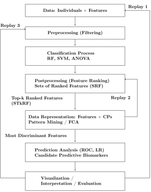
We detail our original knowledge discovery approach for identifying fea-tures which discriminate and predict in the best way classes of individuals in a metabolomic case-control study. This global hybrid and exploratory approach to mining metabolomic data is shown in Figure 1. It combines various al-gorithms for feature selection, supervised and unsupervised classification, and feature ranking. The approach is based on p supervised classification processes, namely CPipi “ 1, . . . , pq, where each CPiis composed of three main operations,
namely preprocessing, classification and postprocessing. Preprocessing is used for preparing the data (filtering) and reducing the feature sets (i.e. reducing the dimensionality of the dataset). Postprocessing is used to rank the features
selected by the classifiers. The different operations composing a classification process as well as the numbers of processes CPi are depending on preferences
of domain experts.
A first challenge is to identify features enabling a good and meaningful sepa-ration between classes of individuals, i.e. cases from controls. The CPi
classifica-tion processes output p sets of ranked features referred to as SRFipi “ 1, . . . , pq
for “Sets of Ranked Features”. Then in each SRFi, the top-k features are
se-lected, where k is set by the analyst. The resulting sets of top-k features are referred to as ST kRFipi “ 1, . . . , pq for “Sets of Top-k Ranked Features”.
These two main operations involve a change of representation space and should be made explicit:
Individuals ˆ F eatures ÝÑ SRFipi “ 1, . . . , pq
SRFi, i “ 1, . . . , p ÝÑ ST kRFipi “ 1, . . . , pq
The classification problem applies first to a dataset Individuals ˆ F eatures and produces p sets of ranked features SRFipi “ 1, . . . , pq. Then, the problem is
transformed as a pattern mining problem, i.e. mining the most frequent features among p sets of top-k ranked features ST kRFipi “ 1, . . . , pq. Then, finding
these features is considered as a pattern mining problem, where a frequency threshold σF is set by the analyst. A feature whose frequency is at least σF in
ST kRFipi “ 1, . . . , pq should appear at least σFtimes in the set of ST kRFipi “
1, . . . , pq. The most frequent features are considered as potentially interesting discriminant features.
It should be noticed that k, i.e. the number of features considered in each SRFipi “ 1, . . . , pq, and σF, the frequency threshold used for mining the
ST kRFipi “ 1, . . . , pq sets are determined by the analyst.
The resulting reduced subset of most frequent features is used as input data for prediction. The prediction capabilities of the selected features are deter-mined thanks to a ROC analysis, which also measures the capability of the approach to discover relevant features and thus predictive biomarkers.
Practically, the change of representation space can be read and visualized using FCA. After construction of the sets SRFi and ST kRFi, a context is built
where rows correspond to features (f ti) and columns to classifiers (CPj). A
cross appears in a cell pi, jq of the context each time the feature f ti is a top-k
feature for the classifier CPj. Then, a concept lattice is built for visualizing
and interpreting the distribution of the most frequent features f ti w.r.t. the
classifiers CPj, i.e. the frequency of f tishould be greater than σF. A complete
use-case following all these steps is detailed in the next section.
As already discussed in the introduction, this knowledge discovery process is hybrid and exploratory, guided by an analyst who is an expert of the domain of data. Hence, interaction and iteration are allowed and they can be read along the “backward arrows” denoted by “Replay” in Figure 1. Actually there are many replay possibilities and here we draw only three of them, that we make precise below.
Data: Individuals ˆ Features
Preprocessing (Filtering)
Classification Process RF, SVM, ANOVA
Postprocessing (Feature Ranking) Sets of Ranked Features (SRF)
Top-k Ranked Features (STkRF)
Data Representation: Features ˆ CPs Pattern Mining / FCA
Most Discriminant Features
Prediction Analysis (ROC, LR) Candidate Predictive Biomarkers
Visualization /
Interpretation / Evaluation
Replay 1
Replay 2 Replay 3
Figure 1: An original hybrid and exploratory approach to mining metabolomic data. The knowledge discovery process is guided by an analyst who is an expert of the domain of data. Interaction and iteration can be read along the backward arrows denoted by “Replay”. Among many possible replays, only three of them are drawn here, and they are related to modification of the process based on the outputs of the knowledge discovery process.
“Replay 1” is a kind of global replay where the analyst wants to modify the data at hand, changing either the set of objects or the set of attributes, based on the current evaluation of the experiment. Usually, the set of objects remains constant within one experiment but the set of attributes can vary, depending
also on the thresholds associated with preprocessing and feature selection. “Replay 2” is related to the setting of two important thresholds, namely k in “top-k” and σF. The threshold k denotes the number of features considered
in each SRFi (sets of ranked features) for forming the ST kRFi (sets of
top-k rantop-ked features). The threshold σF denotes the global frequency used for
extracting the most frequent and potentially discriminant features from the alternative data representation “F eatures ˆ CP s”.
Finally “Replay 3” is related to the choice and the building of the classi-fiers still based on the interpretation results. The analyst may need alternative classifiers, for example in modifying preprocessing (use of alternative filtering methods or setting of different thresholds) and postprocessing (use of alterna-tive measures) and in selecting different classifiers such as neural networks or gradient boosting (e.g. XGBoost).
Actually, the backward arrows “Replay” exemplify the exploratory dimension of the knowledge discovery process and are fully integrated within such a process.
4. The Hybrid and Exploratory Mining of Metabolomic Data in Prac-tice
In this section, we discuss the application2 of our hybrid and exploratory
knowledge discovery approach to metabolomic data. The objective is to find predictive metabolomic biomarkers of T2D development. Due to clinical needs, only a small set of significant features is required for a good separation between cases and controls, and subsequent prediction.
4.1. The Metabolomic Dataset
The dataset under analysis is based on a case-control study within the GAZEL French population-based cohort (20000 subjects). This reference dataset includes 111 male subjects (54-64 years old) free of T2D disease at the initial-ization of the analysis. A binary variable is related to the target class and takes the values “healthy” or “not healthy”. The latter applies to individuals who developed the disease five years after the initial analysis. At the follow-up, 55 subjects developed T2D and belong to the class “not healthy” (diabetic individuals) while 56 belong to the class “healthy” (controls).
Three thousand features are generated for each individual after carrying out mass spectrometry analysis (numerical values of peak intensities). After noise filtration, 1195 features are retained for describing each individual.
4.2. Discrimination Analysis
To identify the discriminant features, 10 classifiers (CPs) are built, composed of three main operations, preprocessing (filtering), classification and postpro-cessing (ranking).
2All experiments were carried out on a Dell computer running Ubuntu 14.04 LTS, a 3.60
GHZ ˆ 8 CPU and 15, 6 GBi RAM. The data analysis methods are taken from RStudio software environment (Version 0.98.1103, R 3.1.1).
4.2.1. Preprocessing
Firstly we consider the original metabolomic dataset with 1195 features and we apply the filtering methods “Cor” (correlation coefficient) and “MI” (mu-tual information). We set two thresholds σCor “ 0.95 and σM I “ 0.02 for the
correlation coefficient and mutual information respectively to eliminate highly correlated and dependent features. Following some related studies, “MI” is as-sociated with the SVM classifier while “Cor” is asas-sociated with the RF classifier [14, 36]. Two reduced sets are then generated: a first set contains 963 features after “Cor” filtering, while a second set contains 590 features after “MI” filtering. In both cases, thresholds have to be adapted for keeping a substantial set of fea-tures to analyze. Then both reduced sets are used as inputs for the classification step.
4.2.2. Postprocessing
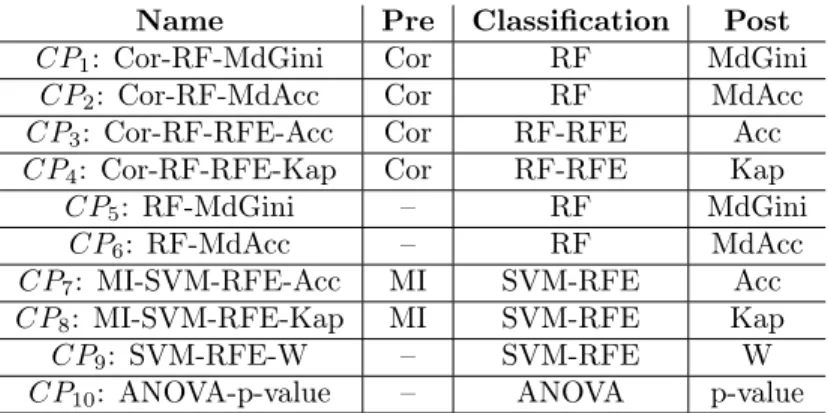
Several measures of interest, namely MdGini, MdAcc, Accuracy (Acc), the weight magnitude of features “W”, and Kappa, are used to assess the importance of features after classification. The general idea is to measure the decrease in accuracy after permutation of the features. The scores given by these metrics allow a ranking of the features for each classifier. The different combinations of these measures among the 10 classifiers can be visualized in Table 1.
4.2.3. Classification
Among the 10 classifiers, one is based on ANOVA and p-value, six are based on RF and three are based on SVM. To improve the classification process, RF and SVM are combined with “Recursive Feature Elimination” (RFE [26]). Four classifiers do not make use of preprocessing while all classifiers make use of postprocessing. The list of classifiers is given in Table 1, where the name of the classifier includes the elementary operations the classifier is made of.
The application of these 10 different classifiers produces 10 different sets of ranked features, denoted by SRFipi “ 1, . . . , 10q. In these 10 SRFiwe select the
100 first ranked features in each CP output, obtaining 10 sets of top-k (k “ 100) ranked features denoted by ST kRFipi “ 1, . . . , 10q. The threshold of 100 has
been set in agreement with domain experts, as sufficiently high for catching the common relevant information among the CPs and sufficiently low for retaining a reasonably sized set of features to interpret.
Below we explain how the analysis of the content of these 10 sets of top-k ranked features was carried out.
4.2.4. The Change of the Data Representation Space
The set of features appearing at least once among the first 100 features for any classifier CPipi “ 1, . . . , 10q is composed of 178 features. Then, a different
data representation space is built, made of a binary table whose dimensions are 178 (features) ˆ 10 (CPs), where objects in rows correspond to features and attributes in columns correspond to the 10 classification processes CPi.
Every feature has a “support w.r.t. the classifiers” between 1 and 10, where in this particular case the “support” counts the number of CPs ranking the
Name Pre Classification Post CP1: Cor-RF-MdGini Cor RF MdGini
CP2: Cor-RF-MdAcc Cor RF MdAcc
CP3: Cor-RF-RFE-Acc Cor RF-RFE Acc
CP4: Cor-RF-RFE-Kap Cor RF-RFE Kap
CP5: RF-MdGini – RF MdGini
CP6: RF-MdAcc – RF MdAcc
CP7: MI-SVM-RFE-Acc MI SVM-RFE Acc
CP8: MI-SVM-RFE-Kap MI SVM-RFE Kap
CP9: SVM-RFE-W – SVM-RFE W
CP10: ANOVA-p-value – ANOVA p-value
Table 1: The 10 classification processes. The name of a classifier includes the elementary operations composing the classifier, i.e. preprocessing, classifier, and postprocessing.
Figure 2: The distribution of the features and their “supports w.r.t. classifiers”. The ordinate axis denotes the number of features and the abscissa axis denotes their support value in terms of CPs. 178 features are top-k ranked by at least one classifier (k “ 100), 48 features are top-k ranked by at least 6 classifiers, and finally 4 features are top-k ranked by all the classifiers.
feature among the 100 first features. Then, the search for the most discriminant features can be carried out following pattern mining principles. Figure 2 shows the distribution of feature support w.r.t. the 10 classifiers, where the ordinate axis denotes the number of features and the abscissa axis denotes their support value. We can check that 178 features have a support of 1, 48 features have a support of 6, i.e. they appear in the 100 best ranked features for at least 6 CPs, and finally 4 features have a maximal support of 10, i.e. they appear in the 100 best ranked features in all CPs. These most frequent features are interpreted as the most interesting discriminant features.
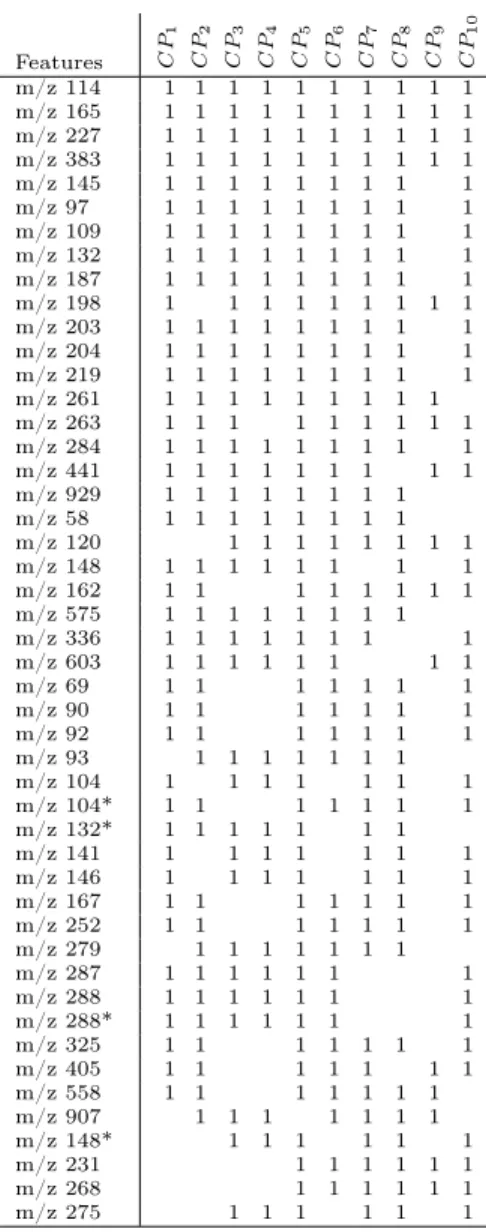
The frequency support was set to 6 in agreement with domain experts, mainly for interpretation reasons and to keep a reasonable number of inter-pretable features. The resulting binary table is shown in Table 2 and is com-posed of 48 features for 10 CPs.
Starting from an initial data table made of 111 (individuals) ˆ 1195 (fea-tures), we obtain firstly 10 sets of ranked features (SRFi, 178 ˆ 10) , and then
Features CP 1 C P2 C P3 C P4 C P5 C P6 C P7 C P8 C P9 C P10 m/z 114 1 1 1 1 1 1 1 1 1 1 m/z 165 1 1 1 1 1 1 1 1 1 1 m/z 227 1 1 1 1 1 1 1 1 1 1 m/z 383 1 1 1 1 1 1 1 1 1 1 m/z 145 1 1 1 1 1 1 1 1 1 m/z 97 1 1 1 1 1 1 1 1 1 m/z 109 1 1 1 1 1 1 1 1 1 m/z 132 1 1 1 1 1 1 1 1 1 m/z 187 1 1 1 1 1 1 1 1 1 m/z 198 1 1 1 1 1 1 1 1 1 m/z 203 1 1 1 1 1 1 1 1 1 m/z 204 1 1 1 1 1 1 1 1 1 m/z 219 1 1 1 1 1 1 1 1 1 m/z 261 1 1 1 1 1 1 1 1 1 m/z 263 1 1 1 1 1 1 1 1 1 m/z 284 1 1 1 1 1 1 1 1 1 m/z 441 1 1 1 1 1 1 1 1 1 m/z 929 1 1 1 1 1 1 1 1 m/z 58 1 1 1 1 1 1 1 1 m/z 120 1 1 1 1 1 1 1 1 m/z 148 1 1 1 1 1 1 1 1 m/z 162 1 1 1 1 1 1 1 1 m/z 575 1 1 1 1 1 1 1 1 m/z 336 1 1 1 1 1 1 1 1 m/z 603 1 1 1 1 1 1 1 1 m/z 69 1 1 1 1 1 1 1 m/z 90 1 1 1 1 1 1 1 m/z 92 1 1 1 1 1 1 1 m/z 93 1 1 1 1 1 1 1 m/z 104 1 1 1 1 1 1 1 m/z 104* 1 1 1 1 1 1 1 m/z 132* 1 1 1 1 1 1 1 m/z 141 1 1 1 1 1 1 1 m/z 146 1 1 1 1 1 1 1 m/z 167 1 1 1 1 1 1 1 m/z 252 1 1 1 1 1 1 1 m/z 279 1 1 1 1 1 1 1 m/z 287 1 1 1 1 1 1 1 m/z 288 1 1 1 1 1 1 1 m/z 288* 1 1 1 1 1 1 1 m/z 325 1 1 1 1 1 1 1 m/z 405 1 1 1 1 1 1 1 m/z 558 1 1 1 1 1 1 1 m/z 907 1 1 1 1 1 1 1 m/z 148* 1 1 1 1 1 1 m/z 231 1 1 1 1 1 1 m/z 268 1 1 1 1 1 1 m/z 275 1 1 1 1 1 1
Table 2: The binary table recording the top-k 48 frequent features w.r.t. the 10 CPs (k “ 100). Each feature is classified among the 100 first features by at least 6 classifiers. Four features have a maximal support. The “m/z” label stands for “mass per charge”. The features are ordered w.r.t. their labels and by decreasing support. Two features such as “m/z 104” and “m/z 104*” for example denote two different molecules with the same nominal mass.
10 sets of frequent top-ranked features with a support of at least 6 (ST kRFi,
48 ˆ 10). The 48 most frequent features are then proposed as candidate for prediction.
Actually, the binary table shown in Table 2 can also be considered as a context in FCA and used for visualizing the distribution of the most frequent features within a concept lattice. A part of the concept lattice –the AOC-poset– corresponding to Table 2 is shown in the next section.
4.3. Prediction Analysis
4.3.1. Identification of Predictive Features and Univariate Analysis
The evaluation of the predictive capability of a feature is measured using a ROC analysis and AUC (area under the ROC curve) [15, 16, 46]. This can be considered as “univariate predictive analysis” because only one feature is con-sidered at a time. The RF classifier was used for carrying out the ROC analysis and for evaluating the predictive capability of the 48 most discriminant fea-tures. More precisely, the data are sampled into a first training set to build the classification model and into a validation set for the estimation of the classifi-cation accuracy. The RF classifier is applied to the subset of 48 features using leave-one-out cross validation and MdAcc to rank the features. A hundred repli-cations of the selection procedure is performed and the output with the lowest misclassification error is retained. A confusion matrix is generated enabling the evaluation of the classification performance w.r.t. six evaluation metrics for ev-ery feature (see Table 3). Various subsets subsets of ranked features are built, denoted by “40-RF”, “30-RF”, “20-RF”, “10-RF” and “5-RF”, which respectively include the 40, 30, 20, 10, and 5 best ranked features. The set “5-RF” is com-posed of the 5 best ranked features by this predictive analysis, namely “m/z 97”, “m/z 145”, “m/z 219”, “m/z 268” and “m/z 325”.
Table 3 summarizes the scores of six evaluation metrics according to RF and MdAcc. The metrics are computed first for the original set of 1195 features and then for the 178 best ranked features extracted from the original 1195 feature set. Then, the metrics are computed for the 48 most discriminant features and then for the reduced feature sets of 40, 30, 20, 10 and 5 best ranked features. It can be noticed that the lowest scores are obtained by the 1195 feature set while the sets with 48 features and less show better performances. However, no feature set is really prominent w.r.t. this predictive analysis.
By contrast, we performed a second experiment using this time Logistic Regression (LR) on the set of 48 features. Logistic regression [16] is commonly used in metabolomics when the number of features under analysis is not too high as this is the case here. LR provided a model with 5 best features, namely “5-LR”, including “m/z 148”, “m/z 167”, “m/z 198”, “m/z 268” and “m/z 288*”. Only one feature, i.e. “m/z 268”, is common to the feature sets “5-RF” and “5-LR”. This highlights that the prediction technique has an influence on the resulting set of best ranked features.
Thus, choosing complementarity rather than separation, the union of both feature sets “5-RF” and “5-LR” including 9 features and termed as “9-RF+LR”
Metrics TPR FPR F-Mes Acc Prec Error Rate 1195-RF 0.81 0.65 0.75 0.73 0.71 0.261 178-RF 0.86 0.82 0.85 0.84 0.84 0.154 48-RF 0.93 0.80 0.88 0.87 0.83 0.131 40-RF 0.85 0.88 0.86 0.87 0.87 0.131 30-RF 0.83 0.90 0.86 0.87 0.90 0.131 20-RF 0.90 0.85 0.88 0.88 0.86 0.119 10-RF 0.85 0.86 0.85 0.85 0.85 0.142 5-RF 0.86 0.85 0.86 0.85 0.86 0.142
Table 3: Six measurements of the performances of feature sets based on the RF classifier. TPR stands for “True Positive Rate”, FPR for “False Positive Rate”, F-Mes for “F-measure”, Acc for “Accuracy”, and Prec for “Precision”.
Name AUC t-tests 95% CI m/z 145 0.795 1.4483E-6 0.657 - 0.896 m/z 97 0.787 1.5972E-6 0.657 - 0.898 m/z 325 0.773 2.2332E-5 0.627 - 0.896 m/z 268 0.759 4.564E-6 0.614 - 0.866 m/z 219 0.712 1.177E-4 0.162 - 0.798 m/z 288* 0.634 0.00499 0.252 - 0.708 m/z 148 0.630 0.01778 0.238 - 0.624 m/z 198 0.619 0.01368 0.197 - 0.594 m/z 167 0.541 0.01796 0.190 - 0.715
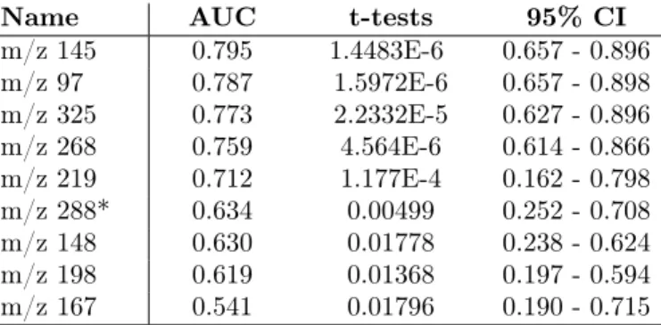
Table 4: Univariate ROC prediction analysis: measuring the performances of the 9 best
features from the set “9-RF+LR” w.r.t. AUC (“area under the ROC curve”) with t-tests
values and confidence interval (CI).
is retained for a ROC analysis. Table 4 presents the ranking of the 9 features w.r.t. their individual AUC value (“Area Under the Curve”) based on the RF classifier. If we only consider features having an AUC higher or equal to 0.75, then 5 features are excluded. The final set of potential predictive biomarkers termed as “4-RF+LR” includes “m/z 145”, “m/z 97”, “m/z 325” and “m/z 268” (ordered by AUC).
Finally, it is interesting to notice that none of the most frequent features, i.e. with a support of 10, is present in this set, and that the support of each feature is respectively 9, 9, 7 and 6. This confirms again that the most discriminant features are not necessarily the most predictive ones.
4.3.2. Multivariate Analysis
Until now, the features are considered separately, as if they were disconnected one from the other, leading to a univariate analysis. However, based on domain practice, biologists and chemists know that, in multifactorial diseases such as T2 diabetes, a combination of markers often helps to better characterize the phenotypes and show very good predictive performances. Following this line, the
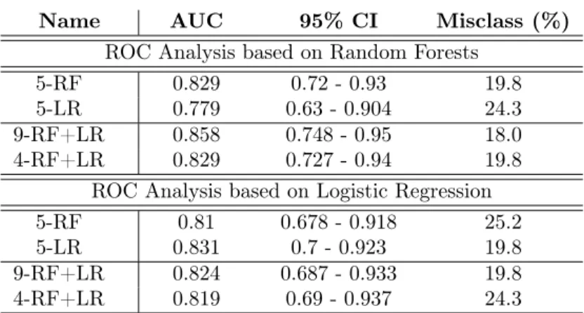
Name AUC 95% CI Misclass (%) ROC Analysis based on Random Forests
5-RF 0.829 0.72 - 0.93 19.8 5-LR 0.779 0.63 - 0.904 24.3 9-RF+LR 0.858 0.748 - 0.95 18.0 4-RF+LR 0.829 0.727 - 0.94 19.8
ROC Analysis based on Logistic Regression 5-RF 0.81 0.678 - 0.918 25.2 5-LR 0.831 0.7 - 0.923 19.8 9-RF+LR 0.824 0.687 - 0.933 19.8 4-RF+LR 0.819 0.69 - 0.937 24.3
Table 5: Multivariate ROC prediction analysis: measuring the prediction capability of the “5-RF”, “5-LR”, “9-RF+LR”, and “4-RF+LR” feature sets.
various sets of predictive features are considered as “a whole” and a multivariate ROC analysis with associated multivariate ROC curves is carried out. The different sets of features are the following:
• “5-RF” = {“m/z 145”, “m/z 97”, “m/z 325”, “m/z 268”, “m/z 219”}, results from ROC analysis and is ranked w.r.t. AUC.
• “5-LR” = {“m/z 268”, “m/z 288*”, “m/z 148”, “m/z 198”, “m/z 167”} results from predictive analysis with logistic regression. and is ranked w.r.t. AUC. • “9-RF+LR” = “5-RF” Y “5-LR” and includes 9 features.
• “4-RF+LR” = {“m/z 145”, “m/z 97”, “m/z 325”, “m/z 268”} excludes 5 features from “9-RF+LR” whose AUC is below 0.75.
The performances of each feature set is shown in Table 5. The ROC analysis is based on two multivariate algorithms, namely RF and LR. The results show an AUC higher than 0.81 for almost all sets of predictive features, except for “5-LR” within ROC analysis based on RF. The performances of this multivari-ate analysis are better than those of the univarimultivari-ate analysis shown in Table 4. Moreover, the set of “9-RF+LR” of predictive features resulting from RF and LR shows the best performance with the lowest misclassification rate (18%), and the highest AUC and CI values according to ROC analysis based on RF. The lowest performance is shown by “5-LR” for ROC analysis based on RF with an AUC of 0.77 and a misclassification rate of 24.3%.
5. Visualization, Interpretation and Validation 5.1. Visualization of Features with FCA
Visualization provides a very good support to data analysis. Considering Table 2 as a binary context, it becomes possible to visualize and analyze the
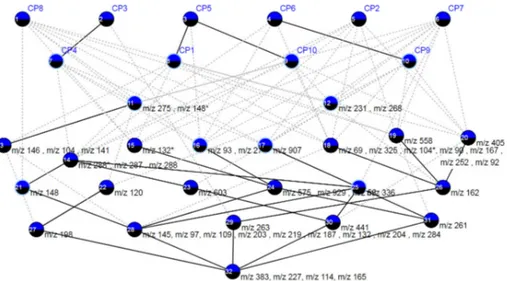
Figure 3: The AOC poset built from the binary table made of the 48 most discriminant features w.r.t. the 10 classification processes. This AOC-poset is drawn thanks to the LatViz system [2], and only includes the so-called “attribute-concepts” and “object-concepts” [17, 6].
resulting AOC-poset [6] which includes all attribute-concepts and all object-concepts (see Figure 3). The AOC-poset includes the “essential elements” of the concept lattice and shows a number of concepts which is much lower than the total number of concepts. The AOC-poset enables to check associations and implications, and the links between the concepts in the lattice represent the dependencies between the features. Checking the AOC-poset from top to bottom, an analyst may appreciate the “support” of a feature w.r.t. the set of classifiers, i.e. the number of classifiers which are ranking the feature among the most frequent, e.g. concepts #11 and #12 are including features with a support of 6. Going down, the support increases until 10 in concept #32 where are lying the four most frequent features “m/z 114”, “m/z 165”, “m/z 227” and “m/z 383”.
We can compare the set of 4 potential biomarkers, namely “m/z 145” (sup-port = 9), “m/z 97” (sup(sup-port = 9), “m/z 325” (sup(sup-port = 7) and “m/z 268” (support = 6), with the four most frequent features (support = 10), i.e. “m/z 114”, “m/z 165”, “m/z 227” and “m/z 383”. Both sets are quite different and this can be explained by the fact that the data are harvested 5 years before the occurrence of the disease. More precisely, in a clear healthy/not healthy design, i.e. a study on samples of an established disease, we could expect at least one or two strong features that would be discriminant and predictive enough to ap-pear as top features. However, in the present study, as samples are harvested 5 years before the occurrence of the disease, metabolomic data may only contain subtle variations linked to the case/control study. Thereby, this could explain the absence of overlap between the two sets of features.
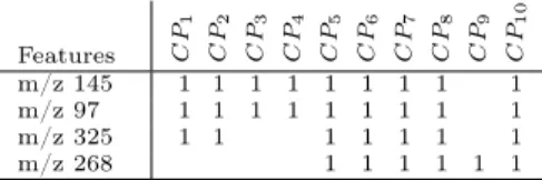
Features C P1 C P2 C P3 C P4 C P5 C P6 C P7 C P8 C P9 C P10 m/z 145 1 1 1 1 1 1 1 1 1 m/z 97 1 1 1 1 1 1 1 1 1 m/z 325 1 1 1 1 1 1 1 m/z 268 1 1 1 1 1 1
Table 6: The binary table describing the 4 best predictive features w.r.t. the 10 CPs.
Figure 4: The concept lattice of the 4 best predictive features.
It should also be noticed that most predictive features do not belong to the same concepts. Features “m/z 145” and “m/z 97” are in concept #28 whose support is 9, i.e. these features are top-100 ranked by all the classifiers but one, namely CP9. By contrast, feature “m/z 325” belongs to concept #18 including 7
CPs, namely CP1, CP2, CP5, CP6, CP7, CP8and CP10, while feature “m/z 268”
belongs to concept #12 including 6 CPs, namely CP5, CP6, CP7, CP8, CP9,
and CP10 (see Table 6). Again, the visualization of the AOC-poset highlights
the distribution of the predictive features among the discriminant (frequent) features and the associations between features and classifiers.
5.2. Interpretation of the Potential of the Classifiers
In this section we would like to characterize the classifiers which have shown good performances in this experiment. Considering the four best features “m/z 145”, “m/z 97”, “m/z 325” and “m/z 268” issued from the ROC analysis, we can build a concept lattice issued from the context given in Table 6, i.e. a part of the largest table 48 features ˆ 10 Cps. The resulting concept lattice is drawn in Figure 4, showing that the top concept includes 5 classifiers, namely CP5,
CP6, CP7, CP8, and CP10, all giving a top ranking to the four features.
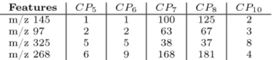
Let us now turn our attention to the 5 classifiers and the way they rank these four features, which is shown in Table 7. RF-based classifiers and ANOVA provide a very good ranking to the 4 features contrarily to CP7 and CP8. It
Features CP5 CP6 CP7 CP8 CP10
m/z 145 1 1 100 125 2 m/z 97 2 2 63 67 3 m/z 325 5 5 38 37 8 m/z 268 6 9 168 181 4
Table 7: The ranking of the 4 best predictive features with respect to 5 CPs.
can be noticed that CP7 and CP8 are SVM-based classifiers which differ only
for postprocessing. Then “m/z 145” is ranked 1st according to CP5 and CP6,
2nd for CP10, and 100th for CP7. The feature “m/z 268” is ranked 6th for CP5,
9th for CP6, 4th for CP10, but 168th for CP7 and 181 for CP8. Thus in this
experiment the identification of biomarkers from metabolomic data seems to be better achieved using RF-based classifiers and ANOVA, both classifiers being complementary.
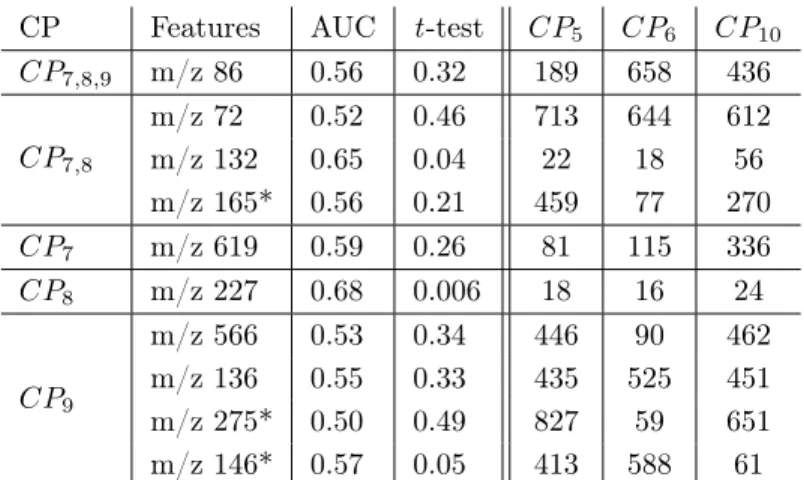
Now, we analyze the differences existing in the ranking of features between RF-based and SVM-based classifiers. We consider the five features with the highest ranking according to SVM-based classifiers and we check how the other classifiers rank them. Table 8 presents the 5 best ranked features according to SVM-based classifiers, CP7, CP8, and CP9, and gives their AUC and t -test
values, as well as their rankings w.r.t CP5, CP6, and CP10(RF without
prepro-cessing and ANOVA classifiers). All features have an AUC value between 0.5 and 0.68, and most of them are poorly classified according to RF and ANOVA. Only two features, namely “m/z 132” and “m/z 227”, have a good ranking for CP5 and CP6, and in addition are frequent (w.r.t. all classifiers) with support
values of 9 and 10 respectively. The other features are not considered as dis-criminant according to RF and ANOVA, and their AUC and t -test values are low.
A first remark is that the use of the weight measure “W” does not seem to be really adapted in this experiment. This can be seen in Table 2, where the column corresponding to CP9is full of empty cells, contrarily to other CP s.
A second remark is that the “Cor” filtering method is very selective and leads to the elimination of some important features, e.g. “m/z 268” which belongs to the core set of 4 potential biomarkers. This is confirmed by Table 2, where the cells for “m/z 268” are empty for the classifiers using the “Cor” filtering, namely CP1, CP2, CP3and CP4. By contrast, “Cor” is not associated to CP7and CP8,
which could explain the different results achieved by SVM-based classifiers. 5.3. Discussion and Validation
The 10 classifiers are based on different algorithms to mine the set of features. ANOVA is based on a simple statistical evaluation metric of variance and is efficient, but this is maybe not sufficient enough to output a small and robust set of best predictive features. We can conclude that combining univariate statistical classifiers with bootstrap-based classifiers can be a relevant choice for mining metabolomic data for discrimination and prediction. Accordingly, a recommendation for data analysts would be first to explore the combination of ANOVA and RF-based classifiers with a preliminary dimensionality reduction
CP Features AUC t -test CP5 CP6 CP10 CP7,8,9 m/z 86 0.56 0.32 189 658 436 CP7,8 m/z 72 0.52 0.46 713 644 612 m/z 132 0.65 0.04 22 18 56 m/z 165* 0.56 0.21 459 77 270 CP7 m/z 619 0.59 0.26 81 115 336 CP8 m/z 227 0.68 0.006 18 16 24 CP9 m/z 566 0.53 0.34 446 90 462 m/z 136 0.55 0.33 435 525 451 m/z 275* 0.50 0.49 827 59 651 m/z 146* 0.57 0.05 413 588 61
Table 8: The performances of the 5 best ranked features according to SVM-based CPs.
of the metabolomic datasets, especially when predictive models are targeted. The following criteria materialize such recommendations and are in agreement with our methodology and the associated results. A much more complete list of specific recommendations for metabolomics is provided in [46]:
1. The combination of univariate and multivariate supervised classifiers is highly recommended.
2. The number of features to select from a classifier should be in agreement with data analysis –thus sufficiently high– and with clinical use –thus not too high– a practical range being the interval r50, 100s.
3. The error rate of the classification models should be inferior to 20%. 4. The AUC value of the best predictive set of features should be above 80%. 5. The AUC value of single features should be above 75%.
From the point of view of the biologists, the use of such an approach en-ables the discovery of patterns or relationships providing useful results and hy-potheses to the experts. Indeed, most of the identified predictive markers have already been shown as modified in early stage of T2D, and are consistent with known metabolic dysregulations (e.g. metabolic syndrome). Moreover, a strat-egy based on large sets of features can be hard to use for discrimination and satisfactory prediction. By contrast, a strategy based on reduced sets of selected features often allow experts to better characterize predictive models, reflecting the metabolic complexity [38].
5.4. A Final Validating Experiment
To confirm the good results of RF and ANOVA for predictive biomarker discovery, we performed another experiment on a different metabolomic dataset from a case-control study including 22 male subjects free of T2D (52-64 years old). The cases consist of 11 subjects who developed T2D at the follow-up and
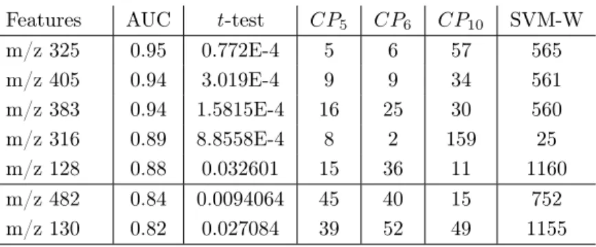
Features AUC t -test CP5 CP6 CP10 SVM-W m/z 325 0.95 0.772E-4 5 6 57 565 m/z 405 0.94 3.019E-4 9 9 34 561 m/z 383 0.94 1.5815E-4 16 25 30 560 m/z 316 0.89 8.8558E-4 8 2 159 25 m/z 128 0.88 0.032601 15 36 11 1160 m/z 482 0.84 0.0094064 45 40 15 752 m/z 130 0.82 0.027084 39 52 49 1155
Table 9: The ranking of the 7 “best features” according to RF+MdAcc classifier.
belong to the class of not healthy individuals. They are compared to controls including 11 subjects who belong to the class of healthy individuals. The dataset is still described by the same 1195 features.
RF, SVM and ANOVA classifiers are applied to this second dataset of 22 individuals ˆ 1195 features. Four sets of ranked features are produced as output w.r.t. the classifiers “RF-MdGini” (CP5), “RF-MdAcc” (CP6), “SVM-W” and
“ANOVA-p-value” (CP10). To identify the best predictive features, the 50
top-ranked features are selected according to the four classifiers. Four reduced sets of top-ranked features are built and then merged to form a final set of 98 features. Then, the predictive capabilities of these 98 features are evaluated with a ROC analysis, including calculation of the AUC, CI and t -test metrics. For doing so, the ROC curves of 3, 5, 10, 20, 49 and 98 features ranked w.r.t. AUC values are examined. The best performance is shown by the whole set of 98 features with an AUC of 0.919. However, the RF-based classifier “RF-MdAcc” (CP6) shows very good performances for 5 top-ranked features with an AUC of
0.877, and with a number of features more adapted to clinical tests.
Two top-ranked features are also selected in a classifier based on LR with an AUC of 0.90, and a misclassification error equal to 9%. The combination of LR and RF produces 7 best predictive features shown in Table 9. The rankings show the similar results achieved by “RF-MdGini” (CP5) and “RF-MdAcc” (CP6), and
a relative complementarity with “ANOVA-p-value” (CP10). Moreover, SVM
shows lower performances but this also confirms that the predictive capability of a classification model is very dependent on the classifier which is used.
6. Conclusion
In this paper, we introduce an original hybrid and exploratory knowledge discovery approach for the identification of relevant biomarkers in complex metabolomic datasets. This approach is based on a combination of numerical supervised and symbolic unsupervised classifiers. We applied the approach to a real case study describing individuals and their features to discover predictive biomarkers. We used classifiers such as Random Forests, SVM and ANOVA, for discovering discriminant and predictive features, as well as pattern mining
and Formal Concept Analysis for reducing the sets of interesting features, for visualization and interpretation purposes.
We also detailed the knowledge discovery process in metabolomic data and discussed the different steps, showing the necessity for such a process to be really interactive and iterative, justifying the “exploratory” character. Actually, on a more general level, a straightforward and fully automated process does not seem to be well adapted to knowledge discovery as soon as data are complex, collected from a real-world domain where strong expertise exists. This paper also provides a substantial example of the gradual approach involving analysts in the biomedical world when they are facing discrimination and prediction problems based on real-world data such as metabolomic data.
For future work, we plan new experiments to consolidate the methodology, with different numerical supervised classifiers. We also envision to make a larger use of symbolic pattern mining methods, for example for carrying out a more complete analysis of implications and association rules that can be discovered from the binary tables. In addition, aggregation methods could also provide other symbolic means for analyzing the sets of ranked features and this also remains to be tested.
References
[1] Alam, M., Buzmakov, A., Napoli, A., 2018. Exploratory Knowledge Dis-covery over Web of Data. Discrete Applied Mathematics 249, 2–17. [2] Alam, M., Le, T. N. N., Napoli, A., 2016. LatViz: A New Practical Tool
for Performing Interactive Exploration over Concept Lattices. In: Huchard, M., Kuznetsov, S. (Eds.), Proceedings of the Thirteenth International Con-ference on Concept Lattices and Their Applications (CLA 2016). CEUR Workshop Proceedings 1624. pp. 9–20.
[3] Armstrong, R., Slade, S., Eperjesi, F., 2000. Statistical review – An in-troduction to analysis of variance (ANOVA) with special reference to data from clinical experiments in optometry. Ophthalmic and Physiological Op-tics 20 (3), 235–241.
[4] Bartel, H.-G., Brüggemann, R., 1998. Application of formal concept anal-ysis to structure-activity relationships. Fresenius Journal of Analytical Chemistry 361 (1), 23–28.
[5] Bartel, J., Krumsiek, J., Theis, F. J., 2013. Statistical Methods for the Analysis of High-Throughput Metabolomics Data. Computational and Structural Biotechnology Journal 4, 5.
[6] Berry, A., Gutierrez, A., Huchard, M., Napoli, A., Sigayret, A., 2014. Hermes: a simple and efficient algorithm for building the AOC-poset of a binary relation. Annals of Mathematics and Artificial Intelligence 72, 45– 71.
[7] Bie, T. D., 2013. Subjective Interestingness in Exploratory Data Mining. In: Tucker, A., Höppner, F., Siebes, A., Swift, S. (Eds.), Proceedings of the International Symposium on Advances in Intelligent Data Analysis (XII). Lecture Notes in Computer Science 8207. Springer, pp. 19–31.
[8] Blinova, V. G., Dobrynin, D. A., Finn, V. K., Kuznetsov, S. O., Pankratova, E. S., 2003. Toxicology Analysis by Means of the JSM-method. Bioinfor-matics 19 (10), 1201–1207.
[9] Blockeel, H., 2015. Data Mining: From Procedural to Declarative Ap-proaches. New Generation Computing 33 (2), 115–135.
[10] Breiman, L., 2001. Random Forests. Machine Learning 45 (1), 5–32. [11] Buzmakov, A., Kuznetsov, S. O., Napoli, A., 2014. Scalable Estimates
of Stability. In: Glodeanu, C. V., Kaytoue, M., Sacarea, C. (Eds.), 12th International Conference on Formal Concept Analysis (ICFCA 2014), Cluj-Napoca, Romania. Lecture Notes in Artificial Intelligence 8478. Springer, pp. 157–172.
[12] Buzmakov, A., Kuznetsov, S. O., Napoli, A., 2015. Fast Generation of Best Interval Patterns for Nonmonotonic Constraints. In: Appice, A., Rodrigues, P. P., Costa, V. S., Gama, J., Jorge, A., Soares, C. (Eds.), Proceedings of the European Conference on Machine Learning and Knowledge Discovery in Databases (ECML-PKDD). Lecture Notes in Computer Science 9285. Springer, pp. 157–172.
[13] Cuperlovic-Culf, M., 2018. Machine Learning Methods for Analysis of Metabolic Data and Metabolic Pathway Modeling. Metabolites 8 (4), 2–16. [14] Ding, C., Peng, H., 2005. Minimum Redundancy Feature Selection from Microarray Gene Expression Data. Journal of Bioinformatics and Compu-tational Biology 3 (2), 185–205.
[15] Fawcett, T., 2006. An introduction to ROC analysis. Pattern Recognition Letters 27 (8), 861–874.
[16] Flach, P. A., 2012. Machine Learning. Cambridge University Press. [17] Ganter, B., Wille, R., 1999. Formal Concept Analysis - Mathematical
Foun-dations. Springer.
[18] García, S., Luengo, J., Herrera, F., 2015. Data Preprocessing in Data Min-ing. Vol. 72 of Intelligent Systems Reference Library. Springer.
[19] Gebert, J., Motameny, S., Faigle, U., Forst, C., Schrader, R., 2008. Iden-tifying genes of gene regulatory networks using formal concept analysis. Journal of Computational Biology 2, 185–194.
[20] Grissa, D., Comte, B., Pujos-Guillot, E., Napoli, A., 2016. A Hybrid Data Mining Approach for the Identification of Biomarkers in Metabolomic Data. In: Huchard, M., Kuznetsov, S. O. (Eds.), Proceedings of the Thirteenth In-ternational Conference on Concept Lattices and Their Applications (CLA-2016). Moscow, Russia, pp. 161–174.
[21] Grissa, D., Comte, B., Pujos-Guillot, E., Napoli, A., 2016. A Hybrid Knowl-edge Discovery Approach for Mining Predictive Biomarkers in Metabolomic Data. In: Proceedings of ECML-PKDD 2016 (Part I). Springer, pp. 572– 587.
[22] Grissa, D., Pétéra, M., Brandolini, M., Napoli, A., Comte, B., Pujos-Guillot, E., 2016. Feature Selection Methods for Early Predictive Biomarker Discovery Using Untargeted Metabolomic Data. Frontiers in Molecular Bio-sciences 3 (30).
[23] Gromski, P., Muhamadali, H., Ellis, D., Xu, Y., Correa, E., Turner, M., Goodacre, R., 2015. A Tutorial Review: Metabolomics and Partial Least Squares-Discriminant Analysis–A Marriage of Convenience or a Shotgun Wedding. Analytica Chimica Acta 879, 10–23.
[24] Gromski, P., Xu, Y., Correa, E., Ellis, D., Turner, M., Goodacre, R., 2014. A comparative investigation of modern feature selection and classification approaches for the analysis of mass spectrometry data. Analytica Chimica Acta 829, 1–8.
[25] Guyon, I., Elisseeff, A., 2003. An Introduction to Variable and Feature Selection. Journal of Machine Learning Research 3, 1157–1182.
[26] Guyon, I., Weston, J., Barnhill, S., Vapnik, V., 2002. Gene Selection for Cancer Classification using Support Vector Machines. Machine Learning 46 (1-3), 389–422.
[27] Hilario, M., Nguyen, P., Do, H., Woznica, A., Kalousis, A., 2011. Ontology-Based Meta-Mining of Knowledge Discovery Workflows. In: Meta-Learning in Computational Intelligence. Springer, pp. 273–315.
[28] Holzinger, A., Dehmer, M., Jurisica, I., 2014. Knowledge Discovery and interactive Data Mining in Bioinformatics – State-of-the-Art, future chal-lenges and research directions. BMC Bioinformatics 15 (S-6), I1.
[29] Jansen, J. J., Hoefsloot, H. C., van der Greef, J., Timmerman, M. E., Westerhuis, J. A., Smilde, A. K., 2005. ASCA: analysis of multivariate data obtained from an experimental design. Journal of Chemometrics 19 (9), 469–481.
[30] Kaytoue, M., Kuznetsov, S. O., Napoli, A., Duplessis, S., 2011. Mining Gene Expression Data with Pattern Structures in Formal Concept Analysis. Information Science 181 (10), 1989–2001.
[31] Kuznetsov, S. O., Samokhin, M. V., 2005. Learning Closed Sets of Labeled Graphs for Chemical Applications. In: Kramer, S., Pfahringer, B. (Eds.), Proceedings of the 15th International Conference on Inductive Logic Pro-gramming (ILP). Lecture Notes in Computer Science 3625. Springer, pp. 190–208.
[32] Mamas, M., Dunn, W., Neyses, L., Goodacre, R., 2011. The role of metabo-lites and metabolomics in clinically applicable biomarkers of disease. Arch Toxicol. 85 (1), 5–17.
[33] Meng, C., Zeleznik, O. A., Thallinger, G. G., Küster, B., Gholami, A. M., Culhane, A. C., 2016. Dimension reduction techniques for the integrative analysis of multi-omics data. Briefings in Bioinformatics 17 (4), 628–641. [34] Métivier, J., Lepailleur, A., Buzmakov, A., Poezevara, G., Crémilleux,
B., Kuznetsov, S. O., Goff, J. L., Napoli, A., Bureau, R., Cuissart, B., 2015. Discovering Structural Alerts for Mutagenicity Using Stable Emerg-ing Molecular Patterns. Journal of Chemical Information and ModelEmerg-ing 55 (5), 925–940.
[35] Nguyen, P., Hilario, M., Kalousis, A., 2014. Using Meta-mining to Support Data Mining Workflow Planning and Optimization. Journal of Artificial Intelligence Research (JAIR) 51, 605–644.
[36] Peng, H., Long, F., Ding, C., 2005. Feature Selection Based on Mu-tual Information: Criteria of Max-Dependency, Max-Relevance, and Min-Redundancy. IEEE Transactions on Pattern Analysis and Machine Intelli-gence 27 (8), 1226–1238.
[37] Poelmans, J., Ignatov, D., Kuznetsov, S., Dedene, G., 2013. Formal Con-cept Analysis in Knowledge Processing: A Survey on Applications. Expert Systems with Applications 40 (16), 6538–6560.
[38] Pujos-Guillot, E., Brandolini, M., Pétéra, M., Grissa, D., Joly, C., Lyan, B., Herquelot, É., Czernichow, S., Zins, M., Goldberg, M., Comte, B., 2017. Systems Metabolomics for Prediction of Metabolic Syndrome. Journal of Proteome Research 16 (6), 2262–2272.
[39] Rinaudo, P., Boudah, S., Junot, C., Thévenot, E. A., 2016. biosigner: A New Method for the Discovery of Significant Molecular Signatures from Omics Data. Frontiers in Molecular Biosciences 3 (26).
[40] Saccenti, E., Hoefsloot, H., Smilde, A., Westerhuis, J., Hendriks, M., 2014. Reflections on univariate and multivariate analysis of metabolomics data. Metabolomics 10 (3), 361–374.
[41] Saeys, Y., Inza, I., Larraaga, P., 2007. A review of feature selection tech-niques in bioinformatics. Bioinformatics 23 (19), 2507–2517.
[42] Tan, P.-N., Steinbach, M., Kumar, V., 2006. Introduction to Data Mining. Addison Wesley.
[43] Tukey, J. W., 1977. Exploratory Data Analysis. Addison-Wesley Publishing Company.
[44] van Leeuwen, M., 2014. Interactive Data Exploration Using Pattern Min-ing. In: Holzinger, A., Jurisica, I. (Eds.), Interactive Knowledge Discovery and Data Mining in Biomedical Informatics – State-of-the-Art and Future Challenges. Lecture Notes in Computer Science 8401. Springer, pp. 169– 182.
[45] Vapnik, V., 1998. Statistical Learning Theory. Wiley-Interscience, John Willey & Sons.
[46] Xia, J., Broadhurst, D., Wilson, M., Wishart, D., 2013. Translational biomarker discovery in clinical metabolomics: an introductory tutorial. Metabolomics 9 (2), 280–99.