Toward robust, fast solutions of elliptic equations on complex domains through HHO discretizations and non-nested multigrid methods

HAL Id: hal-03163476

https://hal.archives-ouvertes.fr/hal-03163476

HAL is a multi-disciplinary open access archive for the deposit and dissemination of sci-entific research documents, whether they are pub-lished or not. The documents may come from teaching and research institutions in France or abroad, or from public or private research centers.

L’archive ouverte pluridisciplinaire HAL, est destinée au dépôt et à la diffusion de documents scientifiques de niveau recherche, publiés ou non, émanant des établissements d’enseignement et de recherche français ou étrangers, des laboratoires publics ou privés.

Toward robust, fast solutions of elliptic equations on

complex domains through HHO discretizations and

non-nested multigrid methods

Pierre Matalon, Daniele Di Pietro, Frank Hülsemann, Paul Mycek, Ulrich

Rüde, Daniel Ruiz

To cite this version:

Pierre Matalon, Daniele Di Pietro, Frank Hülsemann, Paul Mycek, Ulrich Rüde, et al.. Toward robust, fast solutions of elliptic equations on complex domains through HHO discretizations and non-nested multigrid methods. 2021. �hal-03163476�

DOI: xxx/xxxx

RESEARCH ARTICLE

Toward robust, fast solutions of elliptic equations on complex

domains through HHO discretizations and non-nested multigrid

methods

D. A. Di Pietro

| F. Hülsemann

| P. Matalon*

| P. Mycek

| U. Rüde

| D. Ruiz

1_{IMAG, University of Montpellier, France} 2_{EDF R&D, Paris-Saclay, France} 3_{CERFACS, Toulouse, France} 4_{FAU Erlangen-Nürnberg, Germany} 5_{IRIT, Toulouse, France}

Correspondence

*Pierre Matalon. Email: matalon@cerfacs.fr

Summary

The use of modern discretization technologies such as Hybrid High-Order (HHO) methods, coupled with appropriate linear solvers, allow for the robust and fast solution of Partial Differential Equations (PDEs). Although efficient linear solvers have recently been made available for simpler cases, complex geometries remain a challenge for large scale problems. To address this problem, we propose in this work a geometric multigrid algorithm for unstructured non-nested meshes. The non-nestedness is handled in the prolongation operator through the use of the 𝐿2 -orthogonal projection from the coarse elements onto the fine ones. However, as the exact evaluation of this projection can be computationally expensive, we develop a cheaper approximate implementation that globally preserves the approximation properties of the 𝐿2-orthogonal projection. Additionally, as the multigrid method requires not only the coarsening of the elements, but also that of the faces, we lever-age the geometric flexibility of polytopal elements to define an abstract non-nested coarsening strategy based on element agglomeration and face collapsing. Finally, the multigrid method is tested on homogeneous and heterogeneous diffusion prob-lems in two and three space dimensions. The solver exhibits near-perfect asymptotic optimality for moderate degrees of approximation.

KEYWORDS:

Partial Differential Equations, Hybrid High-Order, Multigrid, non-nested meshes, 𝐿2-orthogonal projec-tion

1

INTRODUCTION

Hybrid High-Order (HHO) discretizations1have gained growing interest in recent years for the solution of Partial Differential Equations (PDEs). Amongst their seminal features, we can list their application to general polytopal meshes, their yielded approximate as a broken (i.e. piecewise) polynomial of any arbitrary degree, and their optimal orders of convergence. Especially, the flexibility of polytopal methods with respect to the nature and characteristics of the mesh makes HHO a tool of choice to tackle complex geometries: instead of resorting to local refinement to capture a complex region of the mesh, thereby adding a possibly large number of small elements — and thus increasing the computational cost of the solution —, introducing a small number of polyhedral elements can achieve the same geometric accuracy without sensibly altering the mesh granularity. For

similar structural reasons, HHO natively handles hanging nodes and, more generally, non-conforming meshes, by viewing usual element shapes, like tetrahedra or hexahedra, as identically shaped polyhedra with additional vertices. Another built-in and defining feature of the HHO methods is the use, in the formulation of the bilinear form, of a higher-order potential reconstruction operator, which allows the gain of one additional order of approximation compared to similar hybrid methods, like Hybridizable Discontinuous Galerkin (HDG).2,3_{Finally, the capability of HHO methods to adapt their design to the underlying physics allows} for more robust solutions with respect to the problem. Up to this day, HHO methods have been successfully derived for a large variety of problems in fluid dynamics (heterogeneous anisotropic diffusion,4_{incompressible Navier-Stokes,}5_{creeping flows of} non-Newtonian fluids6_{) and structural mechanics (linear and nonlinear elasticity}7,8_{and poroelasticity}9,10_).

HHO methods hinge on degrees of freedom (DoFs) located in elements and on faces, which can be globally viewed as broken polynomials respectively on the mesh and its skeleton. The element-defined DoFs being only locally coupled, they can be expressed, element by element, in function of the DoFs on the faces, and subsequently eliminated from the global HHO linear system. This gives rise to a Schur complement of smaller size where only face unknowns remain. This process is known as static

condensationin the mechanical literature, and the resulting system as a statically condensed system, or trace system, in reference to the mesh skeleton as the support for the set of globally coupled unknowns. The solution of the trace system, yielding the face unknowns, remains the costliest operation, after which the values of the element unknowns can be inexpensively recovered by solving small independent linear systems.

As a consequence, the practical usefulness of HHO discretizations in an industrial context, where reaching very high scales of resolution is critical, depends on the existence of efficient linear solvers for the condensed system. In this paper, we focus on scalar elliptic equations, whose HHO discretizations give rise to trace matrices that are sparse, symmetric and positive-definite. We endeavour to solve large systems of this type by means of a multigrid method. The main difficulty in the design of a geometric multigrid algorithm for a trace system resides in the location of the DoFs associated to the set of unknowns that remain after static condensation, namely, the face unknowns. Supported by the mesh skeleton, the broken polynomials defined by these DoFs are not fitted for standard intergrid transfer operators, applicable to element-defined functions. The classical multigrid methods that are widely used with standard Finite Elements methods (or any discretization whose DoFs are element-based) are therefore excluded. A literature review of trace system solvers shows the variety of paths one can follow to tackle this particular setting. The first such multigrid algorithm11_{aims at converting the face-defined polynomials to element-defined} ones via the adjoint of the trace operator in order to make use of a known standard geometric multigrid. A variant12 _using this time an algebraic multigrid instead of a geometric one was also experimented. Later, a different approach13 _{is considered} through the design of an ℎ𝑝-multigrid algorithm for unstructured meshes based, for the first time, on trace functions at every level, where the intergrid operators depend on Dirichlet-to-Neumann maps to preserve energy between levels. Finally, also conserving face-defined polynomials at every level, the latest multigrid algorithm,14_{developed by the present authors and which} this work follows up on, is based on a prolongation operator that internally reverses the static condensation to recover coarse element-defined polynomials, before computing their traces on the fine faces. Prior to detailing this solver, we also point out the efforts made to design 𝑝-multigrid preconditioners for non-elliptic equations,15,16,17_{as well as other techniques such as domain} decomposition18,19_{and nested dissection.}20

Although applicable to other hybrid methods with static condensation, the solver developed in our previous work14_{is, to this} day, the only multigrid method specifically targeting HHO discretizations of elliptic problems, by taking advantage of the higher-order potential reconstruction operator to improve its convergence rate. Additionally, rather than managing higher degrees of approximations by the mean of a 𝑝-multigrid on top of an ℎ-one, high-order polynomials are preserved at every level at the cost of a block smoother relaxing all the unknowns related to the same polynomial. Used as a solver, a near-perfect ℎ-independent convergence rate is exhibited on structured 2D and 3D meshes, as well as robustness with respect to the polynomial degree. However, on complex 3D geometries requiring highly unstructured meshes, the average performance may degrade rapidly with the problem size. Indeed, the algorithm requires a hierarchy of nested meshes (although it is experimentally shown that slightly non-nested meshes do not affect the global performance), and such hierarchies are usually obtained from successive refinements of an initial coarse mesh. This way of building embedded grids has a number of known limitations due to the loss of control over the resulting fine grid: firstly, part of the flexibility offered by unstructured meshes to accurately approximate complex regions may be lost in the implicit geometrical conservation in the fine mesh of the large coarse elements, which imposes that the initial coarse mesh already be a good approximation of the geometry. Having stated this, provided an efficient coarse solver, starting from an initial coarse grid that is nonetheless fine enough to adequately capture the geometry can still offer possibilities of very efficient multigrid implementations, such as Hierarchical Hybrid Grids.21,22_{And to help in this approach, recent techniques}23 based on polynomial mappings of the elements allow to better approximate curved boundaries upon each refinement. Secondly,

in 3D, it is well-known24,25,16,26 _{that most methods of tetrahedral subdivision generate elements of degraded shape quality,} which most often affects the accuracy of the approximate solution as well as the performance of the linear solvers. The nested multigrid method14_{indeed shows high sensitivity to the mesh regularity and therefore poor convergence on unstructured meshes} obtained by tetrahedral refinement. Exploring non-nested grids as an alternative to hierarchies produced by mesh refinement is the purpose of the present work. To that end, and before describing our adaptation of the nested algorithm14_{to non-nested grids,} we state that existing non-nested multigrid methods have been devised for the same motives as ours, although none of them applicable to trace systems of hybrid discretizations: continuous Finite Element Methods (FEM) are mostly targeted27,28,29,30,31 and a recent one has been designed for Discontinuous Galerkin (DG) methods,32closer to our setting.

Compliance to non-nested settings is performed by inserting an additional step in the definition of the prolongation operator: starting with polynomials lying on the coarse faces, the nested version14 begins with the reconstruction of a broken element-defined polynomial on the coarse mesh, which we propose (as already performed in the context of DG discretizations32_{) to} orthogonally project in 𝐿2-norm onto the non-nested fine mesh. In a next step, the trace of the result can be computed on the fine faces. The numerical evaluation of this 𝐿2_{-orthogonal projection operator hinges on the projection of the local coarse basis} functions onto the fine bases, i.e. on the computation of the 𝐿2-inner products of the coarse and fine basis functions over the fine elements. As a direct consequence, the local definition of the functional bases makes the intersections of coarse and fine elements the respective integration supports to these inner products. The prerequisite of computing the geometric intersections between coarse and fine elements can occur as computationally prohibitive. So instead of this exact computation, we propose the implementation of an approximate operator that does not require intersections. We also refer to a previous work33that tackles the practical computation of 𝐿2_{-orthogonal projections as well.}

In a face-defined multigrid method, as the smoother operates on the mesh skeleton, the efficient reduction of the low-frequency components of the error relies on accessing coarse representations of the face-defined polynomials. This implies that faces must be coarsened between levels,14, §4.4.3which is a new constraint imposed to any suited coarsening strategy. Unfortunately, usual agglomeration methods,34 _{typical candidates for the coarsening of unstructured meshes, do not meet this requirement. More} generally, methods that conserve embedded meshes do so by conserving fine faces on the coarse mesh, which goes against this new constraint. This observation points out non-nested methods as suitable alternatives. As such, strategies which build coarse tetrahedra from the fine tetrahedra’s vertices35 seem well-adapted to our problem, as long as the shape quality of the coarse elements is sufficient. This condition drives us towards polytopal coarse elements in order to make use of their shape flexibility to construct high-quality coarse meshes. Methods based on Voronoi diagrams36,37fulfill that purpose, as well as our face coarsening constraint. Nonetheless, we choose to propose another option based on element agglomeration. Indeed, additionally to being easy to understand and implement, these methods also benefit from simple derivations to anisotropic grids.38Thus, we suggest to add to any chosen agglomeration process a step of face collapsing, already used in different fashions.39,40_{Moreover, we will} show that agglomeration-based methods ease the construction of our approximate 𝐿2-orthogonal projection.

Having established the reasons driving us to non-nested settings, this work is organized around the adaptation of the existing nested solver14and its efficient implementation for the purpose of its practical use for the solution of condensed linear systems arising from the HHO discretization of scalar elliptic equations on complex geometries. Thus, we begin by describing in Section 2 the HHO discretization of the diffusion equation as model problem. In Section 3, we recall the ingredients in the construction of the nested multigrid method,14 _{and extend its range of application to non-nested meshes through the use of the 𝐿}2_-orthogonal projection. This approach is validated by numerical tests using independent retriangulations at every levels. Insofar as the newly used 𝐿2_{-orthogonal projection depends, in its exact evaluation, on the expensive computation of the intersections between coarse} and fine elements, we devote Section 4 to the definition of a cheaper approximate operator. We also propose in Section 5 a suited non-nested and polytopal coarsening strategy based on element agglomeration and face collapsing. Finally, numerical tests are presented in Section 6, which demonstrate the optimality of our multigrid method, used as a solver, on 2D and 3D diffusion problems.

2

HHO FORMULATION OF THE DIFFUSION EQUATION

2.1

Model problem

Let Ω ⊂ ℝ𝑑_{, with 𝑑 ∈ {2, 3}, be a bounded polyhedral domain with boundary 𝜕Ω. For 𝑋 a measured subset of Ω, 𝐿}2_{(𝑋) denotes} the space of square-integrable functions over 𝑋, equipped with the inner product (𝑢, 𝑣)_𝑋 ∶=∫𝑋𝑢𝑣, for 𝑢, 𝑣 ∈ 𝐿

2_{(𝑋). Likewise,} [𝐿2_(𝑋)]𝑑_{is equipped with the inner product (𝐮, 𝐯)}

𝑋∶=∫𝑋𝐮⋅ 𝐯, for 𝐮, 𝐯 ∈ [𝐿

spanned by functions of 𝐿2_{(𝑋) whose partial derivatives are also square-integrable, and by 𝐻}1

0(𝑋) its subspace of functions with vanishing trace on the boundary 𝜕𝑋 of 𝑋. We consider the following boundary value problem:

{

−∇⋅ (𝐊∇𝑢) = 𝑓 in Ω,

𝑢= 0 on 𝜕Ω, (2.1)

where 𝑓 ∈ 𝐿2_{(Ω) is a given source term and 𝐊 ∶ Ω → ℝ}𝑑×𝑑_{is the diffusion tensor field, which is assumed to be real, symmetric,} uniformly positive definite and piecewise constant over a fixed partition of Ω into polyhedra. The variational formulation of problem (2.1) reads

Find 𝑢 ∈ 𝐻₀1(Ω) such that

𝑎(𝑢, 𝑣) = (𝑓 , 𝑣)_Ω ∀𝑣 ∈ 𝐻₀1(Ω), (2.2) where the bilinear form 𝑎 ∶ 𝐻1_{(Ω) × 𝐻}1_{(Ω) → ℝ is defined by}

∀𝑣, 𝑤 ∈ 𝐻1(Ω), 𝑎(𝑣, 𝑤) ∶= (𝐊∇𝑣, ∇𝑤)Ω.

2.2

HHO Discretization

This section briefly recalls the standard HHO discretization1, Section 3.1of problem (2.2).

2.2.1

Mesh definition

We consider a mesh (_ℎ,_ℎ) of Ω in the sense of1, Definition 1.4_{, i.e.,}

ℎdenotes the set of polyhedral elements,ℎdenotes the set

of faces, and ℎ ∶= max𝑇∈ℎdiameter(𝑇 ) is the meshsize

1, Def. 1.4_{. In the context of problem (2.2), we further assume that the} diffusion tensor 𝐊 is constant over every element 𝑇 ∈_ℎ, and we denote 𝐊_𝑇 ∶= 𝐊|𝑇 for all 𝑇 ∈ℎ. The faces that lie on the

boundary of Ω are collected inB

ℎ and are referred to as boundary faces. Then,ℎmay be partitioned asℎ∶=ℎB∪

I ℎ, with B ℎ ∩ I ℎ= ∅, where I

ℎdenotes the set of internal faces. For 𝑇 ∈ℎ,𝑇 denotes the set of faces that lie on the boundary of 𝑇 .

Reciprocally, for any face 𝐹 ∈ℎ,𝐹 ∶= {𝑇 ∈ℎ∣ 𝐹 ∈𝑇} denotes the set of elements that have 𝐹 as one of their faces.

2.2.2

Discrete setting

With 𝑚 ≥ 0 given integer, we denote by ℙ𝑚_{(𝑋) the space spanned by the restriction of 𝑑-variate polynomials of total degree}

≤ 𝑚 (in short, of degree 𝑚) to 𝑋 ⊂ Ω. Denote by 𝑘 ≥ 0 the polynomial degree of the skeletal unknowns in the HHO scheme. We introduce the following broken polynomial spaces, respectively supported by the mesh and its skeleton:

𝑈𝑚 ℎ ∶= { 𝑣_ ℎ ∶= (𝑣𝑇)𝑇∈ℎ ∣ 𝑣𝑇 ∈ ℙ 𝑚 (𝑇 ) ∀𝑇 ∈ℎ } for 𝑚 ∈ {𝑘, 𝑘 + 1}, 𝑈_𝑘 ℎ ∶= { 𝑣_ ℎ ∶= (𝑣𝐹)𝐹∈ℎ ∣ 𝑣𝐹 ∈ ℙ 𝑘 (𝐹 ) ∀𝐹 ∈ℎ } ,

from which we build the global space of hybrid variables

𝑈𝑘_ℎ∶={𝑣_ℎ=(𝑣_ ℎ, 𝑣ℎ ) ∈ 𝑈𝑘 ℎ× 𝑈 𝑘 ℎ } .

For all 𝑇 ∈ℎ, its local counterpart is

𝑈𝑘_𝑇 ∶={𝑣_𝑇 =(𝑣_𝑇,(𝑣_𝐹)_𝐹∈ 𝑇 ) ∣ 𝑣_𝑇 ∈ ℙ𝑘_{(𝑇 ), 𝑣} 𝐹 ∈ ℙ 𝑘_{(𝐹 ) ∀𝐹 ∈} 𝑇 } . (2.3)

The homogeneous Dirichlet boundary condition is strongly accounted for in the following subspaces:

𝑈_𝑘 ℎ,0 ∶= { 𝑣_ ℎ ∈ 𝑈 𝑘 ℎ ∣ 𝑣𝐹 = 0 ∀𝐹 ∈ B ℎ } , 𝑈𝑘_ℎ,0∶= 𝑈𝑘 ℎ× 𝑈 𝑘 ℎ,0.

Given the exact solution 𝑢 of (2.2), the element and face unknowns of the HHO method (2.6) can be interpreted as the local 𝐿2 -orthogonal projections of 𝑢 onto the respective mesh elements and faces (refer to1, Eq. (2.34)_{). For all 𝑇 ∈}

ℎ, the local potential reconstruction 𝑝𝑘+1

𝑇 ∶ 𝑈 𝑘 𝑇 → ℙ

𝑘+1_{(𝑇 ) is defined such that, for all 𝑣}

𝑇 = ( 𝑣_𝑇,(𝑣𝐹)𝐹∈𝑇 ) ∈ 𝑈𝑘_𝑇, 𝑝𝑘+1 𝑇 𝑣𝑇 satisfies ⎧ ⎪ ⎨ ⎪ ⎩ (𝐊𝑇∇𝑝 𝑘+1 𝑇 𝑣𝑇,∇𝑤)𝑇 = −(𝑣𝑇,∇⋅ (𝐊𝑇∇𝑤))𝑇 + ∑ 𝐹∈𝑇 (𝑣𝐹,𝐊𝑇∇𝑤⋅ 𝐧𝑇 𝐹)𝐹 ∀𝑤 ∈ ℙ 𝑘+1_{(𝑇 ),} (𝑝𝑘+1 𝑇 𝑣𝑇,1)𝑇 = (𝑣𝑇,1)𝑇, (2.4a) (2.4b) where 𝐧_{𝑇 𝐹} denotes the unit vector normal to 𝐹 pointing out of 𝑇 .

2.2.3

Discretization of the model problem

The global bilinear form 𝑎_ℎ∶ 𝑈𝑘 ℎ× 𝑈

𝑘

ℎ→ ℝ is assembled from elementary contributions as follows: 𝑎_ℎ(𝑢_ℎ, 𝑣_ℎ) ∶= ∑

𝑇∈ℎ

𝑎_𝑇(𝑢_𝑇, 𝑣_𝑇),

where for all 𝑇 ∈ℎ, the local bilinear form 𝑎𝑇∶ 𝑈 𝑘 𝑇 × 𝑈 𝑘 𝑇 → ℝ is defined as 𝑎𝑇(𝑢𝑇, 𝑣𝑇) ∶= (𝐊𝑇∇𝑝𝑘𝑇+1𝑢𝑇,∇𝑝 𝑘+1 𝑇 𝑣𝑇)𝑇 + 𝑠𝑇(𝑢𝑇, 𝑣𝑇). (2.5)

In this expression, the first term is responsible for consistency while the second, involving the bilinear form 𝑠_𝑇∶ 𝑈𝑘_𝑇× 𝑈𝑘_𝑇 → ℝ, is required to ensure stability of the scheme. The design of the stabilization bilinear form 𝑠_𝑇is standard and is not detailed here for the sake of conciseness; see1, Assumption 3.9_{on this subject. The global discrete problem then reads}

Find 𝑢_ℎ∈ 𝑈𝑘_ℎ,0such that 𝑎_ℎ(𝑢_ℎ, 𝑣_ℎ) = ∑

𝑇∈ℎ

(𝑓 , 𝑣𝑇)𝑇 ∀𝑣ℎ∈ 𝑈 𝑘

ℎ,0. (2.6)

2.3

Assembly and static condensation

After fixing bases for the spaces 𝑈𝑘 𝑇, 𝑈

𝑘+1

𝑇 and 𝑈 𝑘

𝐹 for all (𝑇 , 𝐹 ) ∈ ℎ ×ℎ. Considering these bases, the local algebraic

contributions of the bilinear form 𝑎_𝑇 (cf. (2.5)) and of the linear form 𝑈𝑘_𝑇 ∋ 𝑣_𝑇 →(𝑓 , 𝑣𝑇)𝑇 ∈ ℝ are, respectively, the matrix 𝐀_𝑇 and the vector 𝐁_𝑇 such that

𝐀_𝑇 ∶= (_𝐀 𝑇 𝑇 𝐀𝑇𝑇 𝐀_ 𝑇𝑇 𝐀𝑇𝑇 ) , 𝐁_𝑇 ∶= ( 𝐛_𝑇 𝟎 ) , (2.7)

in which the unknowns have been numbered so that element unknowns come first and face unknowns come last; see1, Appendix B for further details. After assembling the local contributions and eliminating the boundary unknowns by a strong enforcement of the Dirichlet boundary condition, we end up with a global linear system of the form

( 𝐀_ ℎℎ 𝐀ℎℎI 𝐀_I ℎℎ 𝐀ℎI I ℎ ) ( 𝐯_ ℎ 𝐯_I ℎ ) = ( 𝐛_ ℎ 𝟎 ) . (2.8)

Since element-DoFs are coupled with each other only through face-DoFs, 𝐀_

ℎℎis block-diagonal, therefore inexpensive to invert.

The static condensation process takes advantage of this property to locally eliminate the element-DoFs: it goes by expressing 𝐯_

ℎ in terms of 𝐯ℎI in the first equation of (2.8):

𝐯_ ℎ = −𝐀 −1 ℎℎ𝐀ℎℎI𝐯 I ℎ + 𝐀 −1 ℎℎ𝐛ℎ, (2.9)

and then replacing 𝐯_

ℎwith its expression (2.9) in the second equation:

( 𝐀_I ℎ I ℎ− 𝐀 I ℎℎ𝐀 −1 ℎℎ𝐀ℎℎI ) 𝐯_I ℎ = −𝐀 I ℎℎ𝐀 −1 ℎℎ𝐛ℎ, (2.10)

thus yielding the so-called statically condensed system. After solving (2.10) for the face unknowns 𝐯_I

ℎ, the element unknowns

are locally recovered by the local counterpart of (2.9):

𝐯_𝑇 = −𝐀−1_{𝑇 𝑇}𝐀_{𝑇 𝐹}

𝑇𝐯𝐹𝑇 + 𝐀

−1

𝑇 𝑇𝐛𝑇, (2.11)

where 𝐯𝑇 denotes the restriction to 𝑇 of 𝐯ℎ, and 𝐯𝐹𝑇 the restriction of 𝐯ℎI to the faces of 𝑇 interior to the domain, completed

by zeros for boundary faces.

3

MULTIGRID METHOD ON NON-NESTED MESHES

The multigrid method presented in this section aims at solving the statically condensed system (2.10). It extends the nested algorithm of our previous work14 _{to non-nested mesh hierarchies. The core of the algorithm lies in the definition of the} prolongation operator, which transfers broken polynomials lying on the coarse skeleton to broken polynomials on the fine one. Consistently with the multigrid literature, we use the subscript𝓁 ∈ {1, … , 𝐿} to index the levels in the mesh hierarchy, and we denote by ℎ_𝓁 the meshsize at level𝓁. We sort the levels so that 𝐿 refers to the finest mesh, whereas 1 corresponds to the coarsest one, i.e. ℎ_𝐿 < ℎ_𝐿−1 <⋯ < ℎ₁. Importantly, we further assume that, from a level𝓁 > 1 to the immediately coarser one

(𝓁 − 1), not only are the elements coarsened, but so are the faces. To ease the notation, the subscripts ℎ_𝓁may be replaced with 𝓁, so that the hierarchy of non-nested polyhedral meshes may be denoted by (𝓁,𝓁)𝓁=𝐿…1.

Now, considering two successive levels𝓁 > 1 (fine) and 𝓁 − 1 (coarse), we define the prolongation operator 𝑃 ∶ 𝑈𝑘

𝓁−1,0

→

𝑈_𝑘

𝓁,0

as the composition of three operators,

𝑃 ∶= Π_𝓁◦𝐽_𝓁−1𝓁 ◦Θ_𝓁−1, (3.1)

where the coarse level potential reconstruction operator Θ_𝓁−1∶ 𝑈𝑘

𝓁−1,0

→ 𝑈𝑘+1 𝓁−1

reconstructs, from the face unknowns, a broken polynomial of degree 𝑘 + 1 on_𝓁−1; then, 𝐽𝓁

𝓁−1∶ 𝑈

𝑘+1 𝓁−1

→ 𝑈𝑘+1 𝓁

is now taken equal to the 𝐿2_{-orthogonal projection to include} the non-nested case; finally the trace operator Π_𝓁∶ 𝑈𝑘+1

𝓁

→ 𝑈𝑘

𝓁,0

maps the polynomials of degree 𝑘 + 1 defined on the coarse elements to a broken polynomial of degree 𝑘 on the fine skeleton.

3.1

The potential reconstruction operator

Θ

Given a trace error function 𝑒_

𝓁 ∈ 𝑈

𝑘

𝓁,0 as the operand of Θ𝓁, we recover a element-defined error function in 𝑈

𝑘

𝓁 by locally

reversing the static condensation process. For all 𝑇 ∈𝓁, let us denote by 𝜃𝑇∶ 𝑈_𝑘

𝑇

→ 𝑈𝑘

𝑇 the local operator performing this

operation, as well as 𝑒_

 ∶= (𝑒𝐹)𝐹∈. For all (𝑣𝑇, 𝑣𝑇) ∈ 𝑈

𝑘 𝑇 × 𝑈

𝑘

𝑇, we let 𝐯𝑇 and 𝐯𝑇 ∶= (𝐯𝐹)𝐹∈𝑇 denote their respective

algebraic representations as vectors of coefficients in the selected polynomial bases. With these notations, for all 𝑣_

𝑇 ∈ 𝑈

𝑘

𝑇, the

algebraic representation of 𝑣_𝑇 ∶= 𝜃𝑇𝑣𝑇 is given by the algebraic counterpart of (2.11):

𝐯_𝑇 ∶= −𝐀−1_{𝑇 𝑇}𝐀_𝑇

𝑇𝐯𝑇. (3.2)

Note that the removal of the affine term of (2.11) is justified14, §3.2.1_{by 𝜃}

𝑇 being applied to error functions.

Once the element-defined error 𝑒_𝑇 ∶= 𝜃𝑇𝑒𝑇 is retrieved from (3.2), its accuracy can be improved by one order of

approxi-mation through the use of the higher-order reconstruction operator 𝑝𝑘_𝑇+1 defined by (2.4). Introducing 𝜃_𝑇∶ 𝑈𝑘

𝑇 → 𝑈

𝑘+1

𝑇 such

that for all 𝑣_

𝑇 ∈ 𝑈

𝑘

𝑇,

𝜃_𝑇𝑣_

𝑇 ∶= (𝜃𝑇𝑣𝑇, 𝑣𝑇),

the local contribution to Θ_𝓁is finally given by

(Θ_𝓁𝑒_

𝓁)|𝑇 ∶= 𝑝

𝑘+1

𝑇 𝜃𝑇𝑒𝑇. (3.3)

Note that, although this step of higher-order reconstruction is optional for the convergence and algorithmic scalability of the multigrid method, it improves the convergence rate14, §4.4.1_.

3.2

The trace operator

Π

The trace operator is also locally defined. Let 𝑣 ∈ 𝑈𝑘+1 𝓁

be an element-defined broken polynomial, and 𝐹 ∈ 𝓁. If 𝐹 is a boundary face, then (Π_𝓁𝑣)_|𝐹 is set to be zero; else, (Π_𝓁𝑣)_|𝐹 is built as the weighted average of the traces of 𝑣 on both sides of

𝐹, which is subsequently orthogonally projected onto ℙ𝑘_{(𝐹 ) in order to lower the degree, i.e.}

(Π_𝓁𝑣)_|𝐹 ∶= { 𝑤_𝑇 1𝐹 𝜋 𝑘 𝐹(𝑣|𝑇1)|𝐹+ 𝑤𝑇2𝐹 𝜋 𝑘 𝐹(𝑣|𝑇2)|𝐹 if 𝐹 ∈ I 𝓁, 0 otherwise, (3.4)

where 𝑇₁, 𝑇₂denote the distinct elements in_𝐹 ⊂_𝓁, and 𝜋𝑘 𝐹 is the 𝐿

2_{-orthogonal projector on ℙ}𝑘_{(𝐹 ). Introducing for 𝑖 ∈ {1, 2}}

the scalar coefficients 𝐾_𝑇

𝑖𝐹 ∶= 𝐊𝑇𝑖𝐧𝑇𝑖𝐹 ⋅ 𝐧𝑇𝑖𝐹, the weights are defined as

𝑤_𝑇 𝑖𝐹 ∶= 𝐾𝑇𝑖𝐹 𝐾_𝑇 1𝐹 + 𝐾𝑇2𝐹 . (3.5)

3.3

Multigrid components

Having defined the prolongation operator, the restriction is set to its adjoint in the usual fashion, i.e. with respect to the coarse and fine face-defined global inner products. As such, the matrix of one transfer operator in the chosen polynomial basis is the transpose of the other. Coarse grid operators come from the rediscretization of the problem on the coarse meshes. In order to relax together all the unknowns related to the same local polynomial, block versions of standard fixed point iterations (like

damped Jacobi or SOR) should be used, with a block size corresponding to the number of DoFs per face. For instance, for a 3D problem with the polynomial degree 𝑘 = 1 chosen for the face-defined polynomials, the blocks will be of size 3 × 3. For our numerical tests, the relaxation method is set to the block Gauss-Seidel iteration. In order to keep the computational cost as low as possible, we use the post-smoothing-only cycles that were found to be the most efficient14, §4.2.2_{in terms of total theoretical} work or CPU time. In particular, we use V(0,3) in 2D and V(0,6) in 3D. Finally, on the coarsest level, the system is exactly solved by a direct method.

4

APPROXIMATION OF THE 𝐿

_{-ORTHOGONAL PROJECTION}

In the second step of the prolongation, the global broken polynomial, reconstructed on the coarse mesh from the DoFs on the coarse faces, is projected onto the fine mesh via the 𝐿2_{-orthogonal projection operator denoted 𝐽}𝓁

𝓁−1∶𝓁−1 → 𝓁. The construction of this projection requires the computation of the 𝐿2-inner products of all pairs of coarse/fine basis functions over the fine elements. Locally, one such integral can only be non-zero if the supports of the fine and coarse basis functions intersect, i.e. if the respective fine and coarse elements overlap. In this case, the non-zero part of the integral is restricted to the intersection of the fine and coarse elements.

For any element 𝑇 , we denote by𝑇 the selected basis for ℙ𝑘(𝑇 ). For all 𝑇𝑐 ∈𝓁−1and 𝑇𝑓 ∈𝓁, we then have (𝜑𝑐, 𝜑𝑓)𝑇𝑓 = (𝜑

𝑐_{, 𝜑}𝑓

)𝑇𝑐∩𝑇𝑓 ∀(𝜑

𝑐_{, 𝜑}𝑓

) ∈𝑇𝑐×𝑇𝑓. (4.1)

Consequently, the exact construction of 𝐽𝓁

𝓁−1preliminary requires the computation of the geometric intersection of every pair of overlapping fine/coarse elements. We can see two drawbacks to this method: firstly, the computation of the intersections adds a costly load to the computational burden. Although the actual overhead depends on the efficiency of the algorithm and its implementation, our numerical tests based on the state-of-the-art geometric library CGAL41 _{find it to heavy for practical} use. Secondly, the intersection of usual element shapes, even plain simplices, generally yields a polytope. In practice, if only simplicial meshes are used, one might want to avoid introducing other shapes, over which integral computation may be more expensive.

Given these practical limitations, we introduce a mechanism to compute the operator 𝐽_𝓁−1𝓁 in a cheaper and simpler way, though approximately, by avoiding computing element intersections altogether. It is based on the following approximation (exact when the meshes are nested): For any pair of coarse and fine elements (𝑇_𝑐, 𝑇_𝑓),

𝑇_𝑐∩ 𝑇𝑓 ≈

{

𝑇_𝑓 if 𝑇_𝑐is the coarse element which “embeds 𝑇_𝑓 the most”,

∅ otherwise. (4.2)

According to the element shapes, determining which coarse element embeds the largest part of a given fine one may have multiple interpretations, which may also be implemented in different fashions. For simplicial elements, it suffices to choose the coarse element containing the barycenter of the fine one.

Following this model, each integral over an intersection is either discarded or computed over the whole fine element, in which case the support of the coarse basis function is implicitly extended to include the entire fine element. The number of integrals to compute is then reduced to the number of fine elements.

The validity of this method hinges on the assumption that, if the function to project is smooth enough and if the fine elements

do not stick too much outof the coarse element they are associated to, global approximation properties are preserved. Note that the smoothness requirement emphasizes the restriction not to have elements crossing the boundaries of physical subdomains, i.e. where coefficient discontinuities can occur. Figure 1a shows on a triangulated 2D example how the fine elements are distributed among the coarse ones and how much they can stick out. Graphically, the more the colored clusters of fine elements resemble their respective coarse elements, the less the coarse basis functions must be extended outside of their supports, thus losing accuracy, and therefore the better the approximation of the integrals.

Our numerical tests show that in 2D, on the triangulated square, the approximate operator constructed by this method exhibits good enough accuracy to reproduce the results obtained with the exact computation only for 𝑘 ≤ 1, and fails to be a good approximate for higher orders. In 3D, the method is unsuccessful for all orders. The method is improved the following way: instead of approximating intersections by an all-or-nothing result (either the whole fine element or the empty set) as in (4.2), we can increase the granularity by subdividing the fine elements, and distribute the subshapes among the coarse elements the same way as before. Assuming, for any fine element 𝑇_𝑓 ∈𝓁 a given subdivision Sub(𝑇𝑓), and denoting by closest(⋅) the function

(a) Distribution of the fine elements to their “closest” coarse element.

(b) Distribution of the fine elements’ sub-triangles to their “closest” coarse element.

FIGURE 1 (a) shows the superposition of coarse and fine triangular meshes. The coarse edges are represented by thick black seg-ments. The fine triangles are colored according the coarse triangle they are “closest” to, i.e. the one containing their barycenters. (b) shows the same colored partioning, this time for the fine elements’ sub-triangles.

associating to any element or subelement its “closest” coarse element, we then define the new approximate intersection as

𝑇_𝑐∩ 𝑇𝑓 ≈

⋃

𝑡∈Sub(𝑇𝑓)

closest(𝑡)=𝑇𝑐

𝑡 . (4.3)

Figure 1b shows how sub-triangles obtained by connecting the middle-edges of the fine elements now approach the coarse ones. The fine elements can be refined multiple times for even better accuracy, though at the cost of an increasing number of integrals to compute. However, the approximate operator derived from the fine elements being subdivided only once is found to be sufficient to achieve good multigrid results in 3D and for low polynomial orders. We refer to Section 6.2 for the details of the numerical tests.

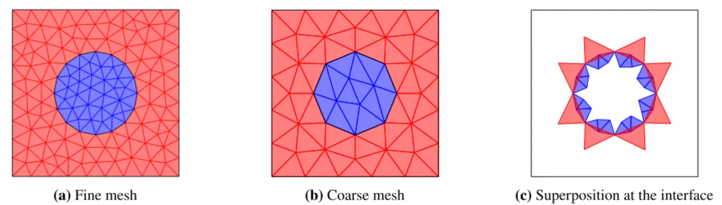
Remark 1. (Heterogeneous case with curved region boundary) If the geometry is partitioned into multiple physical regions with curved boundary, the different levels of grid may approximate this boundary in a non-nested way. Then, imposing that jumps in the coefficient do not occur inside elements inevitably leads to coarse elements overlapping fine ones of different regions. Figure 2 illustrates a two-region domain separated by a circular interface. The approximation of the circle and therefore the discrete delimitation of the regions depend of the granularity of the mesh. Figures 2a and 2b, respectively, show a fine and coarse mesh obtained by Delaunay triangulation, while Figure 2c shows how coarse elements belonging to the red region overlap fine triangles of the blue region. These cases must be handled with great care. In such a configuration, it is crucial that values of DoFs belonging to one region should never be transferred to another one. The 𝐿2-orthogonal projection must then keep this separation. Indeed, the solution cannot be locally represented with accuracy unless it is kept smooth inside elements. In other words, the intersection between a coarse element and a fine one that belong to two different regions must never be computed, and be assimilated to the empty set, even though, in fact, they geometrically overlap. Infringing this guideline results in a quick deterioration of multigrid convergence, and divergence can even occur for small-size problem provided a large jump in the coefficient.

5

AGGLOMERATION-BASED COARSENING STRATEGY WITH FACE COLLAPSING

In this section, we lay the foundations of an abstract coarsening strategy for polytopal meshes that also coarsens faces. The steps are descibed by Algorithm 1. We recall that in this abstract setting, the generic term ‘face’ refers to the interface between elements (it being an actual face in 3D or an edge in 2D), and the term ‘neighbours’ refers to a pair of elements sharing a face. Step 1 is standard and defines any agglomeration method. The face coarsening comes from Step 2, where multiple fine faces are collapsed into a single coarse one. Figure 3 illustates the result of successive coarsenings in 2D. Recall that the created polygons are not necessarily convex. Also, note that this algorithm does not ensure that every fine face is either removed (being interior to an agglomerate) or coarsened (by face collapsing): some fine faces may find themselves unaltered by the process. However,

(a) Fine mesh (b) Coarse mesh (c) Superposition at the interface FIGURE 2 (a) (resp. (b)) presents a fine (resp. coarse) mesh obtained by Delaunay triangulation of a square domain embedding a round physical region. In (c), the red coarse elements overlapping fine blue ones are plotted.

numerical experiments show that the number of unaltered faces between two successive levels decreases with the number of times the coarsening strategy is applied, i.e. the number of levels built.

Algorithm 1 Abstract coarsening strategy with face collapsing

Step 1. Agglomerate each fine element with its non-already agglomerated neighbours to form one polytopal coarse element. Step 2. Collapse into one single coarse face the interfaces between two neighbouring coarse elements that are composed of multiple fine faces.

FIGURE 3 Successive coarsenings of a triangulated square.

Remark 2. (Preventing domain erosion) The face collapsing step removes vertices from the mesh. In order to keep the domain from “eroding” at its corners (whether at domain boundaries or at interfaces between inner regions), one must make sure that the vertices that describe the domain geometry do not vanish in a face collapsing operation. To do so, it suffices to prevent the faces sharing such vertices from collapsing into one coarse face. Applied to a square domain or inner region, it means that at each of the four corners, the two orthogonal corner edges should never collapse together, so that the global squared shape would be preserved.

5.1

Coarsening in 2D

In 2D, the abstract Step 2 can be detailed as such: for all interfaces composed of multiple fine edges, remove all vertices interior to that interface and connect the boundary vertices to form a new coarse edge. This way, we ensure node-nestedness, i.e. that the

set of vertices of the coarse mesh is a subset of the fine vertices. Although having a node-nested hierarchy is not mandatory to achieve good multigrid performance, it may help: assuming that the fine nodes adequately capture the geometry, using subsets of those nodes at coarse levels should present some desirable properties with respect to the geometric approximation.

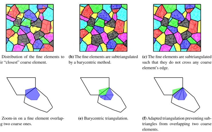
Regarding the computation of the 𝐿2_{-orthogonal projection developed in the preceeding section, numerical experiments show} that the rough approximation given by (4.2) is not viable; see Figure 4a for a graphical illustration. The polygons must be subdivided to improve precision and, clearly, the method of subdivision influences the ultimate accuracy of the approximation. While a barycentric triangulation (Figures 4b and 4e) only offers practical usability for 𝑘 ≤ 1, an optimal triangulation (i.e. yielding an exact approximation; see Figures 4c and 4f) can be derived in the context of a coarsening strategy, inasmuch as the intergrid relationships are explicitly formed and can therefore be exploited. In the present coarsening strategy, the agglomeration step does not cause non-nestedness, which can only occur during the edge collapsing phase. Firstly, only fine elements possessing an edge that has been collapsed and that crosses the coarse collapsed edge must be subject to a careful subdivision; the other fine elements are fully embedded in a coarse one, and therefore do not need to be subdivided at all. Then, for the relevant fine elements, it suffices to generate triangles keeping on one side of the coarse edge. Algorithm 2 presents the details of the optimal subdivision we have used. Note that it applies to convex polygons; the non-convex ones require a preliminary step of convex partitioning before Algorithm 2 can be applied. This algorithm starts by triangulating the polygon independently of the coarse edges. Each triangle is then subtriangulated in order not to cross the coarse edges, following Algorithm 3. Note that this algorithm relies on evaluations of intersections between coarse and fine edges, which node-nestedness can certainly ease, insofar as a large part of the crossings between coarse and fine edges will then occur at mesh vertices.

(a) Distribution of the fine elements to their “closest” coarse element.

(b) The fine elements are subtriangulated by a barycentric method.

(c) The fine elements are subtriangulated such that they do not cross any coarse element’s edge.

(d) Zoom-in on a fine element overlap-ping two coarse ones.

(e) Barycentric triangulation. (f) Adapted triangulation preventing sub-triangles from overlapping two coarse elements.

FIGURE 4 The top figures show how the fine polygons (in (a)) or their subtriangulations (in (b),(c)) are clustered in the process of approximating the coarse/fine intersection involved in the computation of the 𝐿2-orthogonal projection. The coarse edges are represented by thick black segments. In (b), the fine elements are triangulated by a barycentric method. In (c), the triangulation is adapted to prevent subtriangles to overlap multiple coarse elements. The bottom figures zoom in on a fine element overlapping two coarse ones. In (d), the whole fine element is affected to one of them for the computation of the approximate 𝐿2_-orthogonal projection. In (e) and (f), the subtriangles are dispatched on one or the other coarse element according to the location of their barycenters.

Algorithm 2SubdivideConvexPolygon(𝑉 , 𝐸)

Input: 𝑉 : set of vertices sorted in direct order, representing a convex polygon. 𝐸: set of coarse edges not to cross. Output: 𝑇 : set of triangles partitioning the polygon and not crossing the coarse edges.

1: Let (𝑣₁, 𝑣₂, 𝑣₃) be the first 3 vertices in 𝑉

2: 𝑇 ∶= SubdivideTriangle(𝑣₁, 𝑣₂, 𝑣₃, 𝐸) 3: ifcard(𝑉 ) > 3 then

4: 𝑇 ∶= 𝑇 ∪ SubdivideConvexPolygon(𝑉 ⧵ {𝑣₂}, 𝐸) // see Figure 5a 5: end if

Algorithm 3SubdivideTriangle(𝑣₁, 𝑣₂, 𝑣₃, 𝐸)

Input: 𝑣₁, 𝑣₂, 𝑣₃: the vertices of the triangle sorted in direct order. 𝐸: set of coarse edges not to cross. Output: 𝑇 : set of triangles partitioning the triangle and not crossing the coarse edges.

1: if 𝐸= ∅ then 𝑇 ∶= {(𝑣₁, 𝑣₂, 𝑣₃)} // no need to subtriangulate

2: else

3: Let 𝑒 ∈ 𝐸 // take one coarse edge in the list, the others will be handled by recursion

4: 𝑛𝑜𝑇 𝑟𝑖𝑎𝑛𝑔𝑙𝑒𝐸𝑑𝑔𝑒𝐶𝑟𝑜𝑠𝑠𝑒𝑠𝑇 ℎ𝑒𝐶𝑜𝑎𝑟𝑠𝑒𝐸𝑑𝑔𝑒∶= true 5: for 𝑖= 1, 2, 3 do

6: Given 𝑣_𝑖, let 𝑣_𝑗, 𝑣_𝑘be the other two s.t. (𝑣_𝑖, 𝑣_𝑗, 𝑣_𝑘) are in direct order. 7: 𝑊 ∶= 𝑒 ∩ [𝑣𝑖, 𝑣𝑗]

8: if 𝑊 = ∅ or 𝑊 = {𝑣_𝑖} or 𝑊 = {𝑣_𝑗} or 𝑊 = [𝑣_𝑖, 𝑣_𝑗] then continue for loop 9: else

10: 𝑛𝑜𝑇 𝑟𝑖𝑎𝑛𝑔𝑙𝑒𝐸𝑑𝑔𝑒𝐶𝑟𝑜𝑠𝑠𝑒𝑠𝑇 ℎ𝑒𝐶𝑜𝑎𝑟𝑠𝑒𝐸𝑑𝑔𝑒∶= false 11: Define 𝑤 s.t. 𝑊 = {𝑤}.

12: // division into two triangles and recursion; see Figure 5b 13: 𝑇 ∶= SubdivideTriangle(𝑣𝑖, 𝑤, 𝑣𝑘, 𝐸)

14: 𝑇 ∶= 𝑇 ∪ SubdivideTriangle(𝑤, 𝑣_𝑗, 𝑣_𝑘, 𝐸) 15: break for loop

16: end if 17: end for 18: if 𝑛𝑜𝑇 𝑟𝑖𝑎𝑛𝑔𝑙𝑒𝐸𝑑𝑔𝑒𝐶𝑟𝑜𝑠𝑠𝑒𝑠𝑇 ℎ𝑒𝐶𝑜𝑎𝑟𝑠𝑒𝐸𝑑𝑔𝑒 then 19: 𝑇 ∶= SubdivideTriangle(𝑣₁, 𝑣₂, 𝑣₃, 𝐸⧵ {𝑒}) 20: end if 21: end if

5.2

Coarsening in 3D

We have not generalized the preceding coarsening strategy to 3D. Instead, we briefly state the issue and propose directions. In the 3D setting, it is generally not possible to collapse neighbouring faces into a single one as straightforwardly as in 2D, because the edges framing the fine faces do not usually describe a planar region that could define a new face. However, allowing the addition of new vertices, one can derive a variety of face collapsing methods. A simple one consists in choosing three non-colinear vertices amongst those of the fine faces, thus defining a 2D plane, and then orthogonally projecting the frame’s vertices onto that plane to obtain the coarse face. However, in an attempt to preserve, on the coarse mesh, the approximation of the geometry given by the fine one, a more suitable choice for the plane defining the collapsed face would be one minimizing the distance to the vertices lying on the edge frame of the fine faces.

𝑣₁ 𝑣₂ 𝑣₃ 𝑣₁ 𝑣₂ 𝑣₃ 𝑣₁ 𝑣₂ 𝑣₃

(a) First three steps of the triangulation of a convex polygon.

𝑣_{𝑖 𝑣}

𝑗 𝑣𝑘

𝑤

(b) Division of a triangle according to the intersection between the red coarse edge and the triangle edge [𝑣_𝑖, 𝑣_𝑗]. FIGURE 5 Respective illustrations for Algorithm 2 and Algorithm 3.

6

NUMERICAL RESULTS

6.1

Experimental setup

The numerical tests presented in this section have been performed on the diffusion problem (2.1), on 2D and 3D domains, where the source 𝑓 ∈ 𝐿2(Ω) is a discontinuous piecewise constant function. The unit square and cube shall be used as preliminary tests before moving on to more complicated domains. The problems are discretized by the HHO method described in Section 2, in which the polynomial degree 𝑘 of the element- and face-defined polynomials is taken between 0 and 3. We recall that the discrete solution ultimately provided by the method after higher-order reconstruction is a broken polynomial of degree 𝑘 + 1. The local polynomial bases in elements and on faces are 𝐿2-orthogonal Legendre bases.

The multigrid method defined in Section 3.3 is used as a solver for the solution of the statically condensed system (2.10), and our main goal is to study its asymptotic behaviour so that it can be used for large scale problems. The fine mesh is obtained by Delaunay triangulation of the domain, and coarse meshes are built until the system reaches a maximum size of 1000 unknowns or if the mesh cannot be coarsened anymore. Two different strategies are employed to build the coarse meshes: (i) independent remeshing: letting ℎ be the meshsize of the fine simplicial mesh, the coarse mesh is obtained independently by retriangulation of the domain, enforcing a meshsize 𝐻 ≈ 2ℎ; (ii) for 2D problems, the agglomeration-based coarsening strategy with face collapsing, described in Section 5. Table 1 summarizes, for each strategy, the various methods evaluated in the numerical tests to compute the 𝐿2-orthogonal projection. The stopping criterion is based on the backward error‖𝐫‖₂∕‖𝐛‖₂, where 𝐫 denotes the residual of the algebraic system, 𝐛 the right-hand side, and‖⋅‖₂the standard Euclidean norm on the vector space of coordinates. In all tests, we say that convergence is achieved when the criterion‖𝐫‖₂∕‖𝐛‖₂<10−8_{is reached.}

Coarsening strategy 𝐿2-orthogonal projection

Independent simplicial remeshing

Exact, by computing intersections (cf (4.1)) Approximate, w/o subtriangulation (cf (4.2))

Approximate, w/ subtriangulation (cf (4.3)) by middle-edge connection in 2D, Bey’s method in 3D

Agglomeration w/ face collapsing

Exact, by computing intersections (cf (4.1))

Approximate, w/ barycentric subtriangulation (cf (4.3) and Figure 4e) Exact = Approximate w/ optimal subtriangulation (cf (4.3) and Figure 4f) TABLE 1 Summary of the testing combinations.

6.2

Assessment of the approximate 𝐿

_-projection

We want to assess how the loss of accuracy implied by the approximate 𝐿2_{-orthogonal projection (see Section 4) affects the} convergence of the multigrid solver. In order not to add other difficulties that would interfere with the results, we use the unit

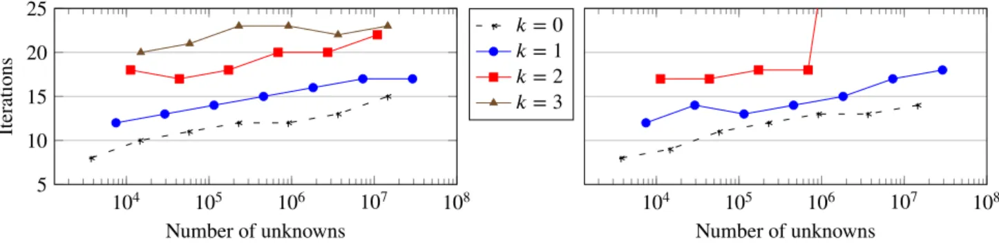
square as domain of study. The coarse meshes are built independently from each other by retriangulation of the domain, ensuring good quality at every level. As a reference to the best achievable result, a first test is made with the 𝐿2_{-orthogonal projection} operator computed exactly, meaning that the intersections of fine and coarse elements are actually computed, over which the required inner products are evaluated (as per (4.1)). Our implementation uses the CGAL library41 _{to compute intersections.} In this first setting, Figure 6a shows, for all polynomial degrees 𝑘, the scalable behaviour of the solver, whose convergence rate appears to be independent of the number of unknowns. The number of V(0,3)-cycles required to achieve convergence remains moderate (below 20), although higher than with nested meshes.14, Fig. 4.5_{This first experiment shows the validity of our} non-nested approach to multigrid.

104 ₁₀5 ₁₀6 ₁₀7 ₁₀8 5 10 15 20 25 Number of unknowns Iter ations 𝑘= 0 𝑘= 1 𝑘= 2 𝑘= 3

(a) Exact 𝐿2_{-orthogonal projection}

104 ₁₀5 ₁₀6 ₁₀7 ₁₀8 Number of unknowns

(b) Approximate 𝐿2_{-orthogonal projection with} subtriangula-tion

FIGURE 6 Number of V(0,3)-cycle iterations to achieve convergence according to the number of unknowns in the system. The geometry is the unit square, and the hierarchy of meshes is obtained by independent remeshing. Each caption states the method of computation of the 𝐿2-orthogonal projection.

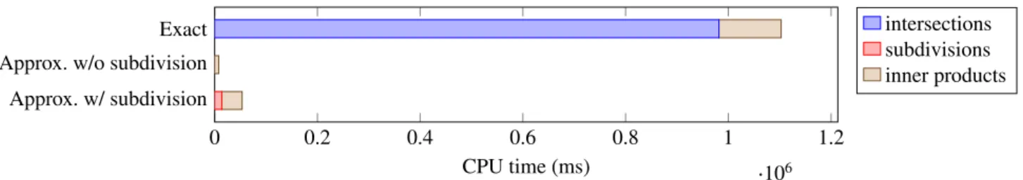
It is important to mention that — in our implementation — the computation of the intersections consumes for 𝑘 = 1 over 80% of the CPU time used during the setup phase. The approximate 𝐿2_{-orthogonal projection we propose allows to reduce} the setup cost by a factor of 10 to 40, depending on the granularity of the fine element subdivisions. As an example, Figure 7 compares, for a test problem with 𝑘 = 1, the CPU time consumed to compute the 𝐿2_{-orthogonal projection, according to the} method used: exact evaluation, approximate without subdivision (given by (4.2)), approximate with subdivision (given by (4.3)). One can clearly see that the largest share is spent in the exact evaluation of the intersection, which makes approximate methods remarkably more effective.

In order to assess the usability of our approximate methods, we now compare to the first scalability results the performance of the solver delivered by our approximations. The approximate 𝐿2_{-orthogonal projection without subdivision (i.e. (4.2)) shows,} in 2D, a lack of robustness w.r.t. the polynomial degree. Although the approximation does not seem to degrade the convergence rate for 𝑘_{≤ 1, it worsens with 𝑘 = 2, and the solver finally diverges for 𝑘 = 3. Moreover, the same test performed in 3D on the}

0 0.2 0.4 0.6 0.8 1 1.2

⋅106 Exact

Approx. w/o subdivision Approx. w/ subdivision

CPU time (ms)

intersections subdivisions inner products

FIGURE 7 Comparison in CPU time of different methods for the computation of the 𝐿2_{-orthogonal projection during the setup} phase of the multigrid. Each bar is divided into sections corresponding to subtasks. The test problem is the unit square meshed by 105_{triangles, 𝑘 = 1.}

unit cube causes the solver to diverge for all values of 𝑘, and so does the use of the 2D polygonal coarsening strategy defined in Section 5. These limitations make us discard this simple method.

We next focus on the finer approximation (4.3), where the fine elements are subdivided into subshapes to increase the granular-ity of the fine-coarse associations. In our tests, we use standard refinement methods to subdivide simplicial elements: connection of the middle-edges in 2D, and Bey’s tetrahedral refinement42_{in 3D. Figure 6b presents the performance of the multigrid solver} on the unit square using this refined 𝐿2_{-orthogonal projection. We can see that the results given by the exact method are now} reproduced. On the unit cube (Figure 8), the solver exhibits good performance and scalable behaviour for 𝑘≤ 2, but diverges for 𝑘 = 3. Note that these 3D results cannot be compared to those of the exact method, as the latter has not been implemented.

104 ₁₀5 ₁₀6 ₁₀7 ₁₀8 10 15 20 25 Number of unknowns Iter ations 𝑘= 0 𝑘= 1 𝑘= 2 𝑘= 3

FIGURE 8 Number of V(0,6)-cycle iterations to achieve convergence according to the number of unknowns in the system. The geometry is the unit cube, which is independently retriangulated at each level. The 𝐿2-orthogonal projection is computed approximately with subtriangulation of the fine elements via Bey’s method.

6.3

Assessment of the agglomeration coarsening strategy with face collapsing

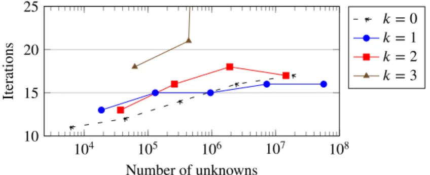
We now evaluate how the multigrid method responds to the coarsening strategy described in Section 5, especially when coupled to the approximate 𝐿2_{-orthogonal projection. Figure 9 then presents the same scalability tests as the previous section, this time} using the agglomeration coarsening with face collapsing to successively build the coarse meshes from an initial fine triangulation. As a reference, Figure 9a shows the results when the 𝐿2_{-orthogonal projection is computed exactly. We can already remark that} the convergence rate is slightly worse and the trend slightly less flat than with the independent remeshing (cf Figure 6a). Various reasons can explain these differences, the main one probably being the simplicity of implementation of our coarsening strategy, where we do not control and subsequently improve the element shapes and sizes.

Algorithmic scalability tests with the 𝐿2_{-orthogonal projection approximately computed without subdivision of the fine} ele-ments are not presented here: except for 𝑘 = 0, the solver quickly diverges. In Figure 9b, we use the barycentric triangulation to subdivide the fine elements (cf Figure 4e) and implement the approximation (4.3). We can see that the good perfomance of

𝑘= 1 is now recovered, while for 𝑘 = 2, the solver still diverges at moderate problem sizes. Finally, we stress that in the context of the corsening strategy, the determination of an optimal fine subtriangulation (i.e. whose subelements do not overlap the limits of the coarse elements) is facilitated, which yields an exact implementation of the 𝐿2-orthogonal projection, and therefore leads to results equivalent to Figure 9a.

6.4

Highly unstructured test cases

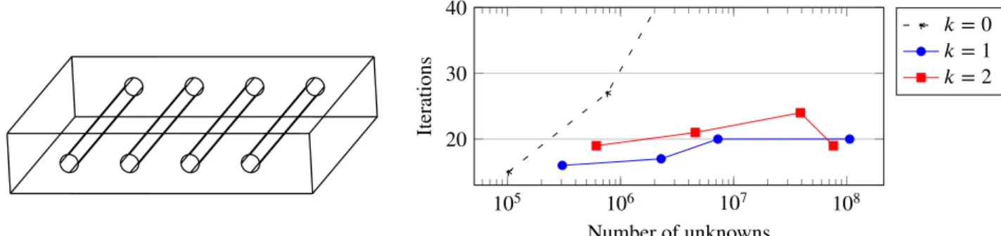
We now extend the experiments to geometries requiring highly unstructured meshes in order to validate the method on a wider class of problems. Figures 10a and 11a respectively draw similar geometries in 2D and 3D containing circular (resp. cylindric) holes, thus requiring highly unstructured meshes in their discrete settings. Still focusing on the capablility of the multigrid solver to handle large scale problems, Figures 10b and 11b present the respective algorithmic scalability plots of the solver. Starting from a fine simplicial mesh obtained by Delaunay triangulation, the coarse meshes are built using the coarsening strategy with face collapsing for the 2D tests, and by independent remeshing for the 3D tests. Notice that, whichever the method, the holes

104 ₁₀5 ₁₀6 ₁₀7 ₁₀8 5 10 15 20 25 Number of unknowns Iter ations 𝑘= 0 𝑘= 1 𝑘= 2 𝑘= 3

(a) Exact 𝐿2-proj., or approximate w/ optimal subtriangulation

104 ₁₀5 ₁₀6 ₁₀7 ₁₀8 Number of unknowns

(b) Approximate 𝐿2-proj. w/ barycentric subtriangulation FIGURE 9 Algorithmic scalability plots: number of V(0,3)-cycle iterations to achieve convergence according to the problem size. The geometry is the unit square. The coarse meshes are built using the agglomeration coarsening strategy with face col-lapsing. The captions state the method of computation for the 𝐿2_{-orthogonal projection. The absence of the curve 𝑘 = 3 in (b)} means a very large number of iterations or divergence of the solver.

are approximated, at each level, with respect to the mesh granularity, i.e. by polygons/polyhedra with less and less edges/faces as the mesh grows coarser. The 𝐿2-orthogonal projection is computed exactly in 2D through the construction of an optimal subtriangulation of the elements. In 3D, the 𝐿2_{-orthogonal projection is computed approximately with tetrahedral subdivision} by Bey’s method. The 2D results presented in Figure 10b show that our multigrid method still exhibits the desired scalable behaviour for all 𝑘≤ 3. In 3D, the results of Figure 11b consistently show the same scalable behaviour for expected polynomial degrees, namely 𝑘 = 1 and 2. The case 𝑘 = 0 is a special case14which is not expected to necessarily work on unstructured problems, while the approximation of the 𝐿2_{-orthogonal projection explains the divergence of the solver for 𝑘 = 3 (cf Figure 8} for the test on the unit cube). Although the displayed datapoints have been obtained with Dirichlet boundary conditions, the results with Neumann conditions on the holes, not reported here for the sake of brevity, indicate the same behaviour.

X Y Z

(a) Bar with four circular holes.

104 ₁₀5 ₁₀6 ₁₀7 ₁₀8 10 15 20 25 Number of unknowns Iter ations 𝑘= 0 𝑘= 1 𝑘= 2 𝑘= 3

(b) Algorithmic scalability plot with the V(0,3)-cycle.

FIGURE 10 2D complex geometry and associated algorithmic scalability plot for the multigrid solver. The coarse meshes are built using the agglomeration coarsening strategy with face collapsing. The 𝐿2-orthogonal projection is computed exactly.

6.5

Heterogeneous test case

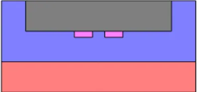
The algorithm is finally tested on a heterogeneous domain, plotted in Figure 12a. This test case, provided by Electricité de France (EDF), is a proxy application for an industrial setting, which is characterized by jumps in the diffusion coefficients of several orders of magnitude in an otherwise relatively straightforward geometry. The proxy differs from the industrial setting in its geometry and its diffusion coefficients. However, the most salient feature, the ratio between the largest and the smallest diffusion coefficient, is close to the relevant regime. The domain is composed of four homogeneous and isotropic subdomains.

X Y

Z

(a) Plate with four cylindric holes.

105 ₁₀6 ₁₀7 ₁₀8 20 30 40 Number of unknowns Iter ations 𝑘= 0 𝑘= 1 𝑘= 2

(b) Algorithmic scalability plot with the V(0,6)-cycle. Elements Hybrid DoFs Face unknowns

(system size) Multigrid levels Iterations Asymptotic convergence rate 17,848,483 177,511,492 106,117,560 5 20 0.45

(c) Details on the last datapoint of 𝑘 = 1.

FIGURE 11 3D test case using the geometry (a). The algorithmic scalability plot (b) of the solver is obtained with the coarse meshes independently retriangulated at each level, and the 𝐿2_{-orthogonal projection computed approximately using Bey’s} subdivision.

Having assigned a color to each of those regions, their respective diffusion tensors 𝜅_color𝐼, where 𝐼 denotes the identity matrix of dimension 2, define a global discontinuous tensor. The values of the coefficients 𝜅colorare given in the caption of Figure 12a and lead to a maximum jump of 108 _{located at the interface between the gray and blue regions. When the coarse meshes} come from independent remeshing of the domain, the scalability plot of Figure 12b demonstrates a convergence rate that is near-independent to the mesh size for all degrees except the lowest order. With the coarsening strategy, on the other hand, (cf. Figure 12c), algorithmic scalability is achieved for all degrees. Moreover, consistently with the results on nested meshes14, §4.3, the convergence rate of the multigrid method is found to be independent of the size of the discontinuities in the coefficient.

Remark 3. (Corner singularities) Heterogeneity in such a domain creates corner singularities which make the discretization lose its optimal convergence rate in the general case. Consequently, although the linear solver converges fast, it converges towards a solution that is not necessarily accurate. It is therefore not imperative to impose the linear solver to reach such a low algebraic error. In order to recover the optimal convergence rate of the discretization, techniques of local mesh refinement or energy correction43_{must be used.}

7

CONCLUSION

In this work, we have successfully extended to non-nested mesh hierarchies an efficient nested multigrid solver. Indeed, without requiring stronger smoothing, our adaptation allows to preserve the optimality of the convergence rate on a wider class of prob-lems. The extra cost implied by the numerical evaluation of the 𝐿2-orthogonal projection is also kept to a minimum thanks to an efficient approximation enabling us to discard the expensive computation of intersections between elements. The agglomeration coarsening strategy with face collapsing that we have developed, although naively implemented here, gives promising results, thus offering leads to more advanced methods fulfilling two purposes: coarsening the faces, and preparing the subtriangulation of the fine elements for the purpose of the construction of an accurate approximation of the 𝐿2-orthogonal projection operator.

ACKNOWLEDGEMENTS

(a) Heterogeneous domain with the coefficients 𝜅red = 30, 𝜅blue= 1, 𝜅gray= 108, 𝜅pink= 100. 103 ₁₀4 ₁₀5 ₁₀6 ₁₀7 ₁₀8 10 20 30 40 Number of unknowns Iter ations 𝑘= 0 𝑘= 1 𝑘= 2 𝑘= 3

(b) Algorithmic scalability plot using independent remeshing.

103 ₁₀4 ₁₀5 ₁₀6 ₁₀7 ₁₀8 Number of unknowns

(c) Algorithmic scalability plot using the coarsening strategy with face collapsing.

Elements Hybrid DoFs Face unknowns (system size) Multigrid levels Iterations Asymptotic convergence rate 18,170,130 109,008,748 54,498,358 9 18 0.40

(d) Details on the last datapoint of (c) 𝑘 = 1.

FIGURE 12 The heterogeneous domain described by (a) is composed of homogeneous, isotropic regions. Their respective diffusion coefficients are given in the caption. In (b), the coarse meshes are built by retriangulation and the 𝐿2_-orthogonal projection is computed approximately with subtriangulation of the fine elements. In (c), the coarsening strategy is used.

References

1. Di Pietro DA, Droniou J. The Hybrid High-Order method for polytopal meshes. Design, analysis, and applications. No. 19 in Modeling, Simulation and ApplicationSpringer International Publishing . 2020

2. Cockburn B, Di Pietro DA, Ern A. Bridging the Hybrid High-Order and Hybridizable Discontinuous Galerkin methods.

ESAIM: Math. Model Numer. Anal.2016; 50(3): 635–650. doi: 10.1051/m2an/2015051

3. Nguyen N, Peraire J, Cockburn B. An implicit high-order hybridizable discontinuous Galerkin method for linear convection-diffusion equations. Journal of Computational Physics 2009; 228(9): 3232–3254. doi: 10.1016/j.jcp.2009.01.030

4. Di Pietro DA, Ern A. Arbitrary-order mixed methods for heterogeneous anisotropic diffusion on general meshes. IMA

Journal of Numerical Analysis2016; 37(1): 40-63. doi: 10.1093/imanum/drw003

5. Botti L, Di Pietro DA, Droniou J. A Hybrid High-Order method for the incompressible Navier–Stokes equations based on Temam’s device. Journal of Computational Physics 2019; 376: 786 - 816. doi: 10.1016/j.jcp.2018.10.014

6. Botti M, Castanon Quiroz D, Di Pietro DA, Harnist A. A Hybrid High-Order method for creeping flows of non-Newtonian fluids. https://arxiv.org/abs/2003.13467; 2020.