Laboratory investigations on the sliding resistance of grounded ice rubble

Publisher’s version / Version de l'éditeur:

Vous avez des questions? Nous pouvons vous aider. Pour communiquer directement avec un auteur, consultez la première page de la revue dans laquelle son article a été publié afin de trouver ses coordonnées. Si vous n’arrivez pas à les repérer, communiquez avec nous à PublicationsArchive-ArchivesPublications@nrc-cnrc.gc.ca.

Questions? Contact the NRC Publications Archive team at

PublicationsArchive-ArchivesPublications@nrc-cnrc.gc.ca. If you wish to email the authors directly, please see the first page of the publication for their contact information.

https://publications-cnrc.canada.ca/fra/droits

L’accès à ce site Web et l’utilisation de son contenu sont assujettis aux conditions présentées dans le site LISEZ CES CONDITIONS ATTENTIVEMENT AVANT D’UTILISER CE SITE WEB.

Technical Report; no. CHC-TR-060, 2009-02-01

READ THESE TERMS AND CONDITIONS CAREFULLY BEFORE USING THIS WEBSITE. https://nrc-publications.canada.ca/eng/copyright

NRC Publications Archive Record / Notice des Archives des publications du CNRC :

https://nrc-publications.canada.ca/eng/view/object/?id=d9c94448-7a3f-4b08-9d3e-19131507557b https://publications-cnrc.canada.ca/fra/voir/objet/?id=d9c94448-7a3f-4b08-9d3e-19131507557b

Archives des publications du CNRC

For the publisher’s version, please access the DOI link below./ Pour consulter la version de l’éditeur, utilisez le lien DOI ci-dessous.

https://doi.org/10.4224/20178993

Access and use of this website and the material on it are subject to the Terms and Conditions set forth at

Laboratory investigations on the sliding resistance of grounded ice

rubble

LABORATORY INVESTIGATIONS

ON THE SLIDING RESISTANCE

OF GROUNDED ICE RUBBLE

Paul Barrette and Garry Timco

TECHNICAL REPORT

CHC-TR-060

LARGE-SCALE LABORATORY INVESTIGATIONS

ON THE SLIDING RESISTANCE

OF GROUNDED ICE RUBBLE

Paul Barrette and Garry Timco Canadian Hydraulics Centre National Research Council of Canada

Ottawa, ON K1A 0R6 Canada

Technical Report CHC-TR-060

ABSTRACT

This report describes an experimental investigation that addresses the resistance to sliding of grounded rubble on a fully saturated sediment bed. It was divided into two phases: in the first one, the sediments consisted of sand; in the second one, a local clay (Leda) was used instead. Testing was done in a concrete flume, 6 by 2.6 m in surface area, located in the CHC ice tank, and incorporating a four-sided enclosure (the ‘wagon’) 2 m by 2 m in surface area, used to contain the ice rubble. The ice was loaded incrementally with concrete slabs, for a total normal stress up to 20 kPa. The wagon was pulled by an actuator over a maximum distance of about 120 mm per test, while the force required to do so was measured with two load cells. Displacement rates ranged from 0.0035 to 0.3 mm/sec. The location of shear failure is believed to have been at the ice-sand interface for all tests. Testing with sand yielded friction coefficients of 0.65 and 0.62, for peak and residual shear stresses, respectively, with the peak response being attributed to dilatation. No effect of displacement rate was noted. Sediment freeze-up at the ice-sand interface increased friction substantially. The clay’s undrained shear strength, measured with a vane, was consistently higher than the sliding resistance of the ice in all tests. The vane data could therefore not be relied upon to provide a measure of sliding resistance. Also, during the test series, this parameter progressively increased to levels well exceeding the maximum normal stress applied to the clay. An alternative approach, based on the soil’s effective internal friction response, is assessed and proposed for estimating sliding resistance of real ice pads and other structures resting on a clay-rich seabed.

RÉSUMÉ

Dans ce rapport, on présente les résultats d’une étude en laboratoire sur la résistance au glissement de la glace en blocailles reposant sur un lit de sédiments saturés. Cette étude comportait deux phases : pour la première, les sédiments étaient constitués de sable; pour la seconde, on a plutôt utilisé une argile locale (argile de « Leda »). Les essais ont été effectués dans un bassin de béton d’une longueur de 6 m et d’une largeur de 2,6 m. Le bassin était situé dans la chambre froide du CHC, et incorporait une enceinte de quatre parois (le ‘wagon’), avec une aire intérieure de 2 m par 2 m et servant à contenir la glace. On a eu recours à des dalles de béton pour charger la glace par incréments, jusqu’à une contrainte normale de 20 kPa. Un vérin mécanique permettait le déplacement du wagon et de son contenu sur une distance maximale de 120 mm par essai. Deux cellules de chargement mesuraient la force requise pour ce déplacement, dont la vitesse était choisie sur une plage allant de 0,0035 à 0,3 mm/sec. Dans tous les cas, on croit que le plan de glissement se situait à l’interface glace-sédiments. Les essais sur sable ont donné lieu à des coefficients de friction de 0,65 et 0,62, pour les contraintes de cisaillement ‘point culminant’ et résiduelle, respectivement, la première étant attribuée au phénomène de dilatation. La vitesse de déplacement n’a pas influencé les résultats. Le gel des sédiments près du contact avec la glace a contribué à augmenter considérablement la résistance au glissement. Pour tous les essais, la résistance non-drainée de l’argile, obtenue au moyen d’une palette, était supérieur à la résistance au glissement de la glace. Les données produites par la palette ne représentaient donc pas une mesure fiable de cette résistance. De plus, les valeurs atteintes progressivement par ce paramètre au cours des essais étaient nettement au-dessus de la contrainte normale maximale appliquée sur l’argile. La friction interne effective de ces sédiments, dont on fait l’évaluation dans ce rapport, pourrait possiblement constituer une alternative pour évaluer la résistance au glissement des plates-formes de glace réelles et autres structures reposant sur le fond marin.

TABLE OF CONTENTS

A

...

R

...

T

C

...

L

F

...

L

T

...

1 I

... 1

2 T

R

... 2

2.1 RATIONALE ... 2

2.2 PURPOSE AND SCOPE... 3

3 E

S

-

... 5

3.1 OVERVIEW OF THE PROCEDURES... 5

3.2 TEST FLUME AND WAGON ASSEMBLY ... 5

3.3 THE SAND ... 7

3.4 THE CLAY ... 7

3.4.1 Potential sources ... 7

3.4.2 Processing... 8

3.4.3 Mechanical characterization ... 8

3.4.4 Consolidation state and shear strength... 8

3.5 THE ICE RUBBLE... 11

3.6 VERTICAL LOADING OF THE ICE ... 12

3.7 THE WATER ... 12

3.8 INSTRUMENTATION... 12

4 S

I

R

S

... 15

4.1 TESTING... 15

4.2 RESULTS ... 16

4.2.1 Shear stress ... 16

4.2.2 Frictional behaviour... 19

4.2.3 Vertical motion of the ice ... 21

4.2.4 Sand bed ... 21

5 S

I

R

C

... 22

5.1 TESTING... 22

5.2 RESULTS ... 22

5.2.1 Shear stress ... 22

5.2.2 Frictional behaviour... 26

5.2.4 Clay bed... 31

6 D

... 34

6.1 TESTING WITH A SANDY SEABED ... 34

6.1.1 Failure location ... 34

6.1.2 Friction coefficients ... 34

6.1.3 Increase in friction resistance with time – compaction... 34

6.1.4 Effects of displacement rate... 34

6.1.5 Sediment freeze-up ... 35

6.2 TESTING WITH A CLAY-RICH SEABED ... 35

6.2.1 Undrained shear strength ... 35

6.2.2 Consolidation state and undrained versus drained conditions during testing ... 35

6.2.3 Vertical motion of the ice ... 36

6.2.4 Shear response ... 36

6.2.5 Dilatancy... 37

6.2.6 Location of shear failure... 38

7 C

... 39

8 A

... 41

9 R

... 42

APPENDIX A – Background information……… A1 APPENDIX B – Clay characterisation……….. B1 APPENDIX C – Reprint of Barrette and Timco (2006)……….. C1

LIST OF FIGURES

Figure 1: Three possible shear planes for global failure. ... 3 Figure 2: Summary of experimental set-up and procedures... 5 Figure 3: a) Test flume inside the CHC ice tank facility; b) Wagon inside the test

flume, before water transfer. Travel direction (arrow) toward the south. ... 6 Figure 4: a) View down the length of the test flume (before the sediments

transfer); b) Pump well inside the longitudinal well, showing the final layout

before testing. ... 7 Figure 5: a) Grinding down the dry Leda clay after it was delivered to CHC;

b) Final state before its transfer into the test flume. ... 9 Figure 6: Laying out the clay in the test flume. Note that the wagon has been

removed from the yellow frame for easier access. ... 9 Figure 7: For the purpose of clay analysis: a) Grab sample; b) Shelby tube; c)

Vane test. ... 10 Figure 8: a) ‘Open’ structure in an unconsolidated clay; b) A reduction in pore

water volume during compression leads to consolidation (with a consequent

increase in shear stress). ... 10 Figure 9: a) Ice ‘trays’ used to produce the ice rubble; b) Layered nature of the

ice inside a rubble tray... 11 Figure 10: a) Rubble ‘generation’; b) Transferring the rubble into the wagon

(using the blue bin shown near the centre of the picture)... 13 Figure 11: a) View of the test flume after the saline water was added; b) Loaded

ice rubble ready for testing on a sand bed (the arrow indicates travel

direction). ... 13 Figure 12: a) One of the two load cells in its waterproof casing; b) Actuator used

to apply a horizontal load to the wagon... 14 Figure 13: Position transducers: a) One unit; b) Layout of the four used for

testing. ... 14 Figure 14: Results for the RS1 test series. The numbers in the legend refer to the

normal stress (in kPa). The two thick lines are for tests done during the

descending sequence of normal stress... 17 Figure 15: Results for the RS2 test series, with no apparent influence of

displacement rate. The normal stress for all tests was about 9.5 kPa... 17 Figure 16: Results for the RS3 test series. The tests are labelled ‘_001’ to ‘_005’,

and the displacement rate of each is indicated in the legend. The normal

stress for all tests was about 8.5 kPa. ... 18 Figure 17: Schematic representation of the shear stress with displacement... 18 Figure 18: Shear stress vs normal stress for the RS1 test series (the test numbers

are indicated). ... 19 Figure 19: Friction coefficients for peak (μp) and residual (μs) shear stresses from

the RS2 test series as a function of displacement rate (DR)... 20 Figure 20: Friction coefficients for RS1, RS2 and RS3 series, in chronological

order. The labels on the x-axis are the test numbers, as indicated in Table 2.

The spike in the sequence is attributed to sediment freeze-up. ... 20 Figure 21: Sand bed at the end of series RS3 (the arrow indicates travel

direction). Glove for scale. ... 21 Figure 22: Results for the RC1 test series for the ascending (a) and descending

stress (in kPa). Note that the test at 13.4 kPa in the descending vertical

sequence was done after an increase in vertical load... 24 Figure 23: Results for the RC2 test series for the ascending (a) and descending

(b) vertical load sequence. The numbers in the legends refer to the total

normal stress (in kPa). ... 25 Figure 24: Results for the RC3 test series, conducted over six days

(normal stress: 3.8 kPa). ... 26 Figure 25: Shear stress vs normal stress for the RC1 test series. The slope of the

linear regression is shown for the ascending sequence the test numbers are

indicated). Green line: overnight period... 27 Figure 26: Shear stress vs normal stress for the RC2 and RC3 test series. The

slope of the linear regression is shown for the ascending sequence (the test numbers are indicated). Green line: overnight period for RC1 and RC2

series... 27 Figure 27: Output from the four position transducers during test series RC1, for

the ascending (a) and descending (b) vertical loading sequences. The labels refer to the normal stress for each test (in kPa). N: North; E: East; S: South; W: West; Average: Dashed line in black. Negative displacement is

downward. ... 28 Figure 28: Output from the four position transducers during test series RC2, for

the ascending (a) and descending (b) vertical loading sequences. The labels refer to the normal stress for each test (in kPa). N: North; E: East; S: South; W: West; Average: Dashed line in black. Negative displacement is

downward. ... 29 Figure 29: Output from the four position transducers during test series RC3 with

a constant vertical load (average normal stress: 3.8 kPa), that ran over six days. N: North; E: East; S: South; W: West; Average: Dashed line in black.

Negative displacement is downward. ... 30 Figure 30: A typical example of a position transducer’s output for one test. ‘A’ is

a nearly flat segment, during which the horizontal displacement is absorbed

by the elasticity of the system. ‘B’ represents the vertical motion... 30 Figure 31: Overnight settlement for three different loads (total concrete mass):

a) 1270 kg; b) 5387 kg; c) 6102 kg. Negative displacement is downward. ... 32 Figure 32: Clay bed after melting off of the ice rubble (meter stick for scale). ... 33 Figure 33: Idealized test sequence summarizing the results discussed in this

paper, with an interpretation of pore pressure dynamics from one test to the next. Leda clay’s effective angle of friction is 30 deg. See text for

LIST OF TABLES

Table 1: Friction coefficients for ice-sediment interaction. n/s: not specified, T: Theoretical study in which a value for this parameter was taken from

elsewhere. ... 2 Table 2: Test grid for the series done with sand. Label ‘B’ in the ‘Concrete mass’

column indicates tests done as part of the descending vertical load sequence... 16 Table 3: Test grid for the series on clay. Displacement rate was 0.03 mm/sec for

all tests. Label ‘B’ in the ‘Concrete mass’ column indicates tests done as

part of the descending vertical load sequence. ... 23 Table 4: Vertical settlements during and between tests. ... 33 Table 5: Friction coefficients produced during these investigations. ... 34

LABORATORY INVESTIGATIONS

ON THE SLIDING RESISTANCE

OF GROUNDED ICE RUBBLE

1 Introduction

Sea ice is submitted to current- and wind-induced loads that causes it to split, collide and break up, ultimately resulting in the formation of ice rubble. Ice rubble also tends to accumulate around structures operating in the offshore environment, such as drilling platforms (e.g. Poplin and Weaver 1992). A significant body of knowledge on this subject was acquired during the 1970’s and 1980’s, when the high cost of exploration in the Canadian and the Alaskan Beaufort Sea called for efficient and innovative methods for stabilizing drilling platforms (Graham et al., 1984; Croasdale et al., 1994). It was found that grounded rubble could effectively protect these installations from the surrounding ice cover in moderate water depths (Potter et al., 1984; CANATEC, 1994; see Barker and Timco, 2005, for a review). The reason is that part of the load transmitted by the surrounding pack ice, either of thermal origin or induced by currents and winds, is absorbed by the grounded rubble, thereby greatly reducing the loads transmitted to the structure (Marshall et al., 1989; Wong et al., 1991; Sayed, 1992; Timco and Sayed, 1993; Timco and Wright, 1999). For instance, this issue was addressed with the Tarsuit Caisson Retained Island (CRI), a shallow-water caisson structure used by Gulf Canada Resources Ltd. in 1981 and 1982 for drilling purposes (see e.g. Timco and Wright, 1999). During the winter 1982-1983, the CRI was left on-site as a test ground for the investigations of ice-structure interactions. At that time, it was surrounded by a grounded rubble field, itself enclosed within landfast first-year sea ice. Three distinct loading events were analysed and it was found that the forces on the outer faces of the caisson were, on average, 38% lower than those measured along the outer edge of the rubble.

Another issue related to offshore winter operations is that of evacuation, whereby crew members may have to leave a structure during an emergency (such as a well blow out), and venture onto the ice (Wright et al., 2003; Timco and Dickins, 2005; Timco et al., 2006). An improved understanding of rubble stability would help determine the best method of escape, especially since a suitable pathway would have to be maintained to access shelters mounted on the ice as part of the evacuation procedures (Barker et al., 2007; Spencer et al., 2007).

The oil and gas sector is currently expressing renewed interest in the hydrocarbon potential below the Beaufort Sea and other ice-covered sea expanses, such as offshore Alaska, China and in the Sakhalin region of Russia. Exploration activity is taking place, or is expected to do so, in the Caspian, Barents and Kara seas. Ice load resistance is a critical design parameter for bottom-founded offshore installations. Reduced design loads, stemming from an adequate understanding of the friction behaviour between ice rubble and the sea bottom, would allow future exploration platforms to be built with increased confidence and at less cost.

2 This Report

2.1 RATIONALE

Resistance to sliding is usually expressed in terms of a friction coefficient, which is the ratio of horizontal to vertical stresses. It is customarily referred to as static if the peak horizontal stress at the onset of sliding is considered, and as kinetic if it is the stress required to keep the ice in motion. A survey of the literature on the friction between ice and sediments (more details of which are presented in Appendix A) is summarized in Table 1. The friction coefficients shown in this table were either generated in the laboratory or the field, or extracted from elsewhere and used in the authors’ calculations. The wide range of values obtained for, or assigned to, this parameter may be attributed to a variation in the size of the interaction, the nature of the ice-sediment interface and the type of ice-sediments, amongst other reasons. The friction coefficient is indeed one of the main sources of uncertainty in the assessment of sliding resistance, which is why it is the focus of the large-scale investigations described herein.

Table 1: Friction coefficients for ice-sediment interaction. n/s: not specified, T: Theoretical study in which a value for this parameter was taken from elsewhere.

Friction coefficients

Source Ice feature Sediment (or _{surface) type} Static Kinetic n/s Size of interface (m2₎ Croasdale and Marcellus (1978)(T) Rubble n/s 0.6 n/s Croasdale et al. (1978) (T) n/s n/s 0.1 – 0.7 n/s Allyn and Wasilewski

(1979) (T) Rubble n/s 0.7 n/s Kovacs and Sodhi

(1980) (T) Small floe Beach 0.6 n/s Utt and Clark (1980) Ice block Silt, sand, gravel 0.85 – 1.23 0.06 Shinde and Wards

(1982) (T) Rubble

Rough wood

planking 0.50 – 0.68 n/s Abdelnour et al.

(1982) Model ice Sand 0.75 < 0.5 Sodhi et al. (1983) (T) Model ice Plywood 0.09 n/s Wards (1983) Saline ice Sands (one frozen),

silt 0.48 – 0.68 0.47 – 0.86 0.1 Wards (1983) Ice rubble Sand 0.46 – 0.98 5 – 10 Shapiro and Metzner

(1987) Sea ice

Unfrozen beach

gravel 0.50 0.39 6 to 8 Kemp et al. (1987) (T) Sea ice Clays 0.65 n/s Gulati (1992) Rubble Sand 0.43 – 0.80 5 (estim.) Weaver and Poplin

(1997) Spray ice island Cohesive Beaufort seabed 0.44 113,000 (real scale) Takeuchi et al. (2003) Saline ice Sand 0.35 – 0.90 0.30 – 0.65 0.007 Barker and Timco

(2003a) Ice block Sand, gravel 0.48 – 0.52 down to 0.22 0.6

Furthermore, the question may arise as to the location of the failure plane. Failure may occur within the ice, along the ice-seabed interface (especially if it is frozen to the ice), or within the seabed (Figure 1). A combination thereof is also possible. This is an issue that was raised with ice pads – when designing these structures, failure of the ice-seabed interface is considered the critical failure mode (e.g. Weaver et al., 1991; Morgan, 2005). But is this always the case, irrespective of the seabed’s strength characteristics? An assessment of this issue can also be addressed in the laboratory.

Finally, if failure does occur at the ice-sediment interface, how do the sediments’ mechanical properties influence the interaction? Sediment strengths and consolidation state in the Beaufort Sea vary significantly. How relevant is this information in the assessment of sliding resistance?

Driving Force

Failure through the ice

Failure at seabed interface

Failure through the seabed

Figure 1: Three possible shear planes for global failure.

2.2 PURPOSE AND SCOPE

The aim of the investigations presented in this report is to generate information on the sliding resistance of ice rubble, particularly with regards to friction behaviour, failure location and influence of soil behaviour. First and foremost, this study addresses the following question: For a given vertical stress onto the seafloor, how much horizontal load is required to reposition the rubble? Although a laboratory approach provides a means a controlling the parameters relevant for this purpose, to date it has failed to deliver consistent data, mainly because of a large variation in test set-ups, procedures and materials used in previous studies. Another constraint typical of a laboratory environment is, of course, the reduced size of the interaction: how representative is it of a full-scale scenario? The experimental program described herein attempts to overcome these limitations while further improving our understanding of this phenomenon. This is done as follows:

ƒ The footprint of the ice mass used in these experiments was of considerable size (4 m2₎ and was meant to reproduce as closely as possible real-scale interaction events. Scaling laws and principles are not involved.

ƒ Normal stresses equivalent to those existing at the base of some installations previously deployed in the Beaufort Sea are attained.

ƒ The experimental program was divided into two phases: one during which sand was used as the sediment bed; the other during which clay was used instead. The test procedures were the same for both phases, thereby affording an opportunity to compare rubble-sediment interactions with two quite distinct materials, under identical conditions. ƒ The vertical settlement of the ice during its travel is monitored.

ƒ Finally, the experimental set-up described herein was also used to study the friction behaviour of a single slab of level ice (as opposed to rubble) on sand{Barrette, 2006 #19 – see Appendix C; Barrette, 2008 #580} and clay (Barrette and Timco, in press, Cold Regions Science and Technology). The data presented in the present report should thus provide a comparative basis for either rubble or level ice, two common types of ice relevant to the design of spray ice pads (bearing in mind that these structures may be built on either of these ice types).

In this report, the experimental set-up is described at first, followed by the data collected with sand and with clay. These results are then discussed separately in the ‘discussion’ section, which is followed by a section outlining the relevance of these results on current offshore engineering issues.

The material dealt with in the report straddles two relatively distinct fields of study: ice and geotechnical engineering. For the readers not familiar with either of these fields, Appendix A provides some background information, as well as references to other works. The topics covered include a concise overview of the origin and nature of ice rubble and some fundamental notions in geotechnical engineering and ice-seafloor interaction. In addition, this appendix presents a review on the physical and mechanical properties of the Beaufort seafloor sediments. Appendix B contains information related with the physical and mechanical properties of the Leda clay used in these investigations. Appendix C is a reprint of a paper published by the authors, which presents earlier data on the sliding resistance of level ice on sand.

3 Experimental Set-up

3.1 OVERVIEW OF THE PROCEDURES

The experimental procedures were divided into three distinct operations (Figure 2): 1. Generation of rubble ice and transfer of that rubble into the wagon;

2. Vertical loading of this ice, meant to simulate the freeboard; and

3. Horizontal loading, meant to reproduce loads of thermal origin or those induced by currents and winds, at a constant displacement rate while monitoring the forces required to do so.

Step 1: Ice rubble transfer in the wagon

Sediments

2 m

Concrete floor and walls

Step 2: Vertical loading of the ice rubble

Wood panel

Step 3: Horizontal loading

Concrete slabs Normal stress up to 20 kPa Measured shear stress up to 9 kPa

Figure 2: Summary of experimental set-up and procedures.

3.2 TEST FLUME AND WAGON ASSEMBLY

The test was set up in the CHC ice tank (Pratte and Timco, 1981), inside which a flume was built for the purpose of this experimental program (Figure 3a). The inside length and width of this flume was 6 and 2.6 m, respectively, with a height of 1.2 m. The walls were 203 mm thick and were made of re-bar reinforced concrete. A removable steel gate at one end of the flume was used

to access the flume’s interior. Guide rails were anchored onto the top of the two longitudinal walls (Figure 3b). These allowed motion of a frame assembly used to carry a four-sided enclosure (the wagon), henceforth collectively referred to as wagon, enclosing the rubble and used to drag it onto the sediment bottom. Each wagon sidewall consisted of a 19 mm-thick Plexiglas sheet 2 m in length and 0.79 m in height screwed onto the wagon’s structural members. The recourse to a transparent material was to allow video sequences of the rubble to be collected during testing. This, however, was not feasible because of the high content of clay-sized particles in suspension, even with sand, which caused the water to be too murky (even after attempts at removing the fine fraction by filtering the water) and impede visibility.

Steel gate Ice tank Test flume West rail Load cells East rail

S

a)

a)

Figure 3: a) Test flume inside the CHC ice tank facility; b) Wagon inside the test flume, before water transfer. Travel direction (arrow) toward the south. The test flume’s floor included a 0.1 m deep and 1 m wide recess running in its centre and along most of its length (Figure 4a). This recess, which was initially intended to accommodate bed load transducers for a future test program, was filled in with gravel, a material that resists compaction. Failure to do so could have resulted in a non-uniform distribution of the bulk strain within the overlying sediments during the forward motion of the loaded ice rubble. The entire floor was then covered with a woven polypropylene geotextile material, whose purpose was to prevent the sediments from penetrating the gravel. To facilitate water transfer in and out of the test flume without excessively disrupting the sediment column, a well that was designed to house a smaller pump (30 litres/min) was installed at one end of the test flume (Figure 4b). This system allowed filling the test flume from the bottom of the sediment column upward. Because it extended down into the central pit, the well also made it easier to drain the sediments after testing.

Figure 4: a) View down the length of the test flume (before the sediments transfer); b) Pump well inside the longitudinal well, showing the final layout before testing.

3.3 THE SAND

The sand was obtained from a quarry in the Ottawa area. D10, D30 and D60 were 0.16, 0.30 and 0.61 mm, respectively, and the angle of repose was 32.5 degrees. The drained shear strength was determined in a direct shear box apparatus. JACQUES WHITFORD was contracted out to carry out direct shear tests. Normal stresses of 15, 30 and 60 kPa, yielded peak shear stresses of 6.5, 23.5 and 51.8 kPa, respectively. This corresponds to a friction angle of about 40 degrees, or

μ = 0.84.

The sand was laid onto the geotextile sheet to a total thickness of about 300 mm, that is, 50 mm below the wagon’s lowest structural member. These procedures were done as part of an earlier test program involving a level ice sheet {Barrette and Timco, 2006 – see Appendix C –, 2008, Barrette et al. in press). After that test program was completed, the sand was mixed and levelled back to a 300 mm level with a rake for the test series dealt with in the present report.

3.4 THE CLAY

3.4.1 Potential sources

The most accessible clay material for these investigations was the Leda clay, “a predominantly marine deposit of post-glacial age which accumulated in an arm of the ocean known as the Champlain Sea” (Gillott, 1971, p. 797), which abounds in the Ottawa Valley. A local contractor working on a construction site in Orleans (located at 45o27’58”N and 75o27’35”W) was asked to deliver a truckload of it to CHC, which was done at no cost. One can take issue on the fact that this clay is “quite unique and by no means would be representative of those under the Beaufort Sea” (K.T. Lau, 2006, writt. comm.). For the purpose of comparison, the results of mineralogical and chemical analyses conducted on that clay as well as on two other clays supplied in a dry form by Canadian manufacturers (PLAINSMAN CLAY LTD, from Medicine Hat, Alberta, and PAISLEY BRICK AND TILE Co., from Paisley, Ontario) are included in Appendix B. These analyses suggest that the ‘Paisley’ sample, with its very high illite content (which is an important

Gravel Gravel

Xsection of longitudinal pit

Sand Sand

Geotextile

Pump Well

Basin’s concrete floor

250 mm

b) a)

component of the Beaufort see clays – see Appendix A), may have been a better choice, if one is concerned about correctly reproducing the shrinking and swelling behaviour of the clay under load. It was decided to closely monitor the Leda clay’s shear strength during the test program, so as to be able to relate this parameter to the measured friction coefficients.

3.4.2 Processing

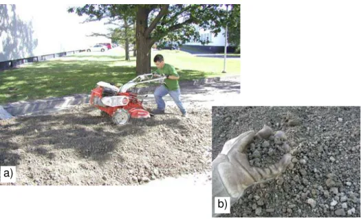
Because of its propensity to form chunks upon drying, the clay required additional care to ensure the end product was reasonably homogeneous. A rototiller was used to reduce the size of the dried up fragments making up the clay pile (Figure 5). This was done repeatedly, for a cumulative amount of time up to 3-4 hours. The transfer to the test flume was done in three steps, following which just enough 27 ppt saline solution was added to submerge it. The first, second and third batches were allowed to soak for three, one and seven days, respectively. Between each step, the clay was spread evenly with a rake and a shovel (Figure 6). After an additional month of soaking, it was then levelled to a thickness of about 300 mm. Because of clay’s low permeability, the pump well used with the sand (Figure 4) was deemed unnecessary and was removed.

3.4.3 Mechanical characterization

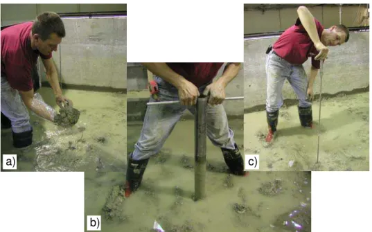
JACQUES WHITFORD was contracted out to conduct mechanical testing of the clay. This was done in three steps. Firstly, moisture content, unit weight, specific gravity, clay content as well as shear strength of the clay were obtained prior to initiating the test program. Grab samples and Shelby tube samples were collected, and vane tests were done for that purpose (Figure 7). Secondly, vane tests were done throughout the test program to monitor changes in shear strength. These were done both within and outside the scoured zone. The third step was to repeat what was done in the first step, in addition to determining the clay’s Atterberg limits. Note that the latter step took place after a later test program (Barrette and Timco, in preparation), such that they are not truly representative of the sediments at the end of the test program described in the present report. All results are shown in Appendix B.

3.4.4 Consolidation state and shear strength

As explained in Appendix A, clay-rich sediments are porous – they have an ‘open’ internal structure that is filled with water under fully saturated conditions. The volume of open space varies according to the amount of normal stress the clay is, or has been, subjected to (Figure 8). The more compacted , the lower its porosity and the higher its shear strength. This is related with its ‘consolidation’ state. When conducting this type of investigations with clay-rich sediments, one may want to ensure that the shear strength of the clay is representative of what it is one is trying to simulate or model. When a target shear strength has been decided upon, the clay may be submitted to a normal pressure (or pre-consolidation) until it has achieved the desired strength. Testing may then proceed.

The present investigations are concerned with the clays on the seafloor of the Beaufort Sea. The mechanical properties of these sediments, however, are not uniform. Jefferies et al. (1985), for instance, report shear strengths ranging from 0 to 50 kPa in the upper 2-3 m offshore the McKenzie delta. Kemp et al. (1987) mention a shear strength of 25 kPa for shallow clays, which was used for the design of the Kadluk ice pad. Weaver et al. (1992) report shear strengths ranging from 0 kPa at the surface to 60 kPa at a depth of 1 m. Since the test program was not designed with any specific geographic location in mind, the average shear strength of 17 kPa obtained at the onset of the test program was deemed adequate, such that a pre-consolidation procedure was not required.

Figure 5: a) Grinding down the dry Leda clay after it was delivered to CHC; b) Final state before its transfer into the test flume.

Figure 6: Laying out the clay in the test flume. Note that the wagon has been removed from the yellow frame for easier access.

a)

Figure 7: For the purpose of clay analysis: a) Grab sample; b) Shelby tube; c) Vane test. a) Unconsolidated

σ

Figure 8: a) ‘Open’ structure in an unconsolidated clay; b) A reduction in pore water volume during compression leads to consolidation (with a consequent increase in shear stress).

c)

b) a)

3.5 THE ICE RUBBLE

A 6 ‰ saline solution was prepared in a large pit inside the CHC ice tank by diluting sodium chloride into tap water. This solution was pumped out of this pit into 15 containers 2.4 m long, 0.4 m wide and 0.3 m deep and with vertical walls (Figure 9a). They were built for that purpose from galvanized steel sheets. The water was added in increments of 20-30 mm and was allowed to freeze at an air temperature of -15oC. This procedure took a few days to complete. The resulting ice was layered (Figure 9b). The air temperature was then raised above freezing point so as to free the ice from the containers’ walls. Doing so, the ice lost most of its brine content: several salinity measurements showed that it did not exceed 1 to 2 ‰. The ice density was not measured; an estimate of 900 kg/m3 was used for the calculation of vertical loads.

Figure 9: a) Ice ‘trays’ used to produce the ice rubble; b) Layered nature of the ice inside a rubble tray.

Next, the ice was taken out of the containers by turning them upside down one by one. A pry bar was used to break it in pieces of various sizes (Figure 10a). These were transferred with a fork lift into the test flume inside the wagon (Figure 3b and Figure 10b).

The total ice volume, obtained by keeping track of the ice dimensions retrieved from each container, was 1.93 m3. A porosity of about 0.20 was estimated on the basis of this volume and that occupied by the rubble inside the wagon. Rubble thickness could be monitored by measuring the distance from the water level to both the top of the rubble and the sand at the base of it. The value for this parameter was 550 to 600 mm at the beginning of the test series, and about 280 mm at the end. This reduction probably resulted from both compaction of the rubble and melting of the ice. The first mechanism contributed in reducing porosity; the second one did the opposite. There was no way of monitoring either process during testing. However, another porosity estimate mid-way during testing yielded a similar value, which suggests that one process compensated the other. Also, the salinity of the water in the flume went down to 25 ‰, which does provide an indication of how much melting occurred. But the information required to assess its extent, including water level at the time of salinity measurement, was not gathered systematically.

b) a)

The procedures described so far were those used for testing on sand. For testing on clay, they were essentially the same, resulting in a similar rubble porosity (0.21). Melted ice specimen yielded salinities of 2.4, 2.4 and 2.6 ‰.

3.6 VERTICAL LOADING OF THE ICE

A series of 10 square-shaped slabs, made from rebar-enforced concrete, was used to apply a vertical load onto the rubble-sediment column. The slabs were 1.8 m in length and width, and had a thickness of 90 mm, for a total mass of about 800 kg, except for the first plate, which was 60 mm in thickness, for a mass of 470 kg. The net vertical load was equal to the total weight of the concrete slabs, the rubble and a plywood board laid on top of the rubble (onto which the slabs were loaded), minus the buoyancy of all submerged elements. The total normal stress was obtained by dividing the net vertical load by the rubble’s footprint (4 m2). The general principles are described in section 3.1 of Appendix A.

3.7 THE WATER

For the first phase of the work (with sand), a 32 ‰ saline solution, at or near the freezing point, was pumped into the flume (Figure 11a). The rubble was levelled and covered with a 40 mm-thick plywood board, which acted as a base onto which the concrete slabs were laid (Figure 11b). The final water level varied from about 280 to 600 mm above the sediment column. As mentioned earlier, a small capacity pump was used to initiate the water transfer. Once the water level reached a significant height above the sediments, a high capacity pump (240 litres/min) was used to complete the operation. The water density was not measured; an estimate of 1025 kg/m3 was used for the calculation of buoyancy.

For the second phase of the work (with clay), the salinity of the water before it was transferred into the test flume was 27 ‰ but eventually went down to 20 ‰ even before testing, perhaps because of the freshwater already present in the sediments.

3.8 INSTRUMENTATION

Two 45 kN capacity load cell in water-proofed casings were mounted in parallel onto the downstream wagon wall (Figure 3b, Figure 12a). They were attached to the bottom of the wagon, as close as possible to the ice-sediment interface in order to minimize the amount of torque exerted onto the rail at the wagon’s suspension points. These cells monitored the load exerted onto the wagon by a steel bar connected to two stainless steel pull rod. The rods extended to, and went through, the flume’s southern wall. Sealed guide tubes in the wall ensured water tightness. On the other side of that wall, the rods were clamped onto a second bar, itself driven by a worm gear actuator (Figure 12b). Two gear box ratios were available: 20:1 and 60:1, but only the latter was used.

The actuator’s maximum travel distance was 124 mm, which was recorded by a position transducer, located on top of the actuator (Figure 12b). As will be seen later, the elasticity of the system accounted for up to 40% of the total displacement. The voltage output from these three channels (two load cells and one position transducer) was recorded and managed with GEDAP, a real-time control software designed by CHC (Miles, 1990; Pelletier, 2001). Data acquisition rate varied from 5 to 100 Hz for the series done with sand. For the experiments done with clay in the second phase of the work, the data was acquired at 1 Hz.

Figure 10: a) Rubble ‘generation’; b) Transferring the rubble into the wagon (using the blue bin shown near the centre of the picture).

Figure 11: a) View of the test flume after the saline water was added; b) Loaded ice rubble ready for testing on a sand bed (the arrow indicates travel direction).

In addition to the two load cells and the position transducer on the actuator, four position transducers were used for testing on clay. These were attached onto the wagon frame on the north, east, south and west side of the concrete load (Figure 13). Extension rods were used when necessary. The position transducers allowed to monitor three degrees of freedom of the rubble:

heaving (vertical motion), pitching (tilting about a horizontal axis at right angle to travel direction) and rolling (tilting about a horizontal axis parallel to travel direction).

a) b)

a)

Position transducer Actuator Gear box Motor

a)

a)

Figure 12: a) One of the two load cells in its waterproof casing; b) Actuator used to apply a horizontal load to the wagon.

Figure 13: Position transducers: a) One unit; b) Layout of the four used for testing. a)

4 Sliding of Ice Rubble on Sand

4.1 TESTING

A total of 26 successful tests, grouped into three series, were conducted for this phase (Table 2): ƒ During the first series (RS1), whose purpose was to find out how the shear stress varied

with normal stresses, each test was done with ascending and descending vertical load – or stress – increments and at a displacement rate of 0.03 mm/sec, chosen on an arbitrary basis. A 470 kg concrete slab was laid onto the plywood board for the first 124-mm test. After test completion, the actuator was brought back to its initial position and another concrete slab was added to the vertical load for the next test, and so on, up to a total concrete mass of about six metric tons, and taking into account the ice/plywood or the buoyancy of all submerged components. This corresponds to an upper bound normal stress of about 14 kPa. At the end of this first test series, the wagon was pulled back to its starting position so as to allow for additional tests. In order to do that, the concrete slabs were removed and the water level raised. At that stage, the rubble was still fairly loose. Additional rubble was added into the wagon. The scoured sand was also raked back to a uniform level. Testing was done with loose rubble, at an ambient air temperature of 2 oC ± 2oC, with up to five tests a day.

ƒ The second series (RS2) was meant to investigate the potential effect of displacement rate on friction behaviour. All tests in this series were done with a total of five concrete slabs, for a normal stress of about 9.5 kPa. The displacement rate for each test varied in a random order. Testing done with loose rubble, at an ambient air temperature of 2 oC ± 2oC.

ƒ For the third series (RS3), the rubble was allowed to consolidate (freeze) by lowering the ambient air temperature to -8oC ± 2oC, and maintaining it to that level for the duration of the test series (seven days). The normal stress was kept constant at about 8.5 kPa. The purpose of this series was to attempt to freeze the sediments below the ice and observe potential changes in the friction behaviour (as briefly discussed in Barrette and Timco, 2006 – see Appendix C). During that time, the concrete mass prevented the monitoring of the freezing front in the underlying rubble. But the thickness of the rubble at the time was relatively thin (280 mm) so it was assumed to be completely frozen.

The thickness of the rubble was monitored before each test of all three series. It was 600 mm at the beginning of RS1 and 280 mm at the end of RS3. The water level was also monitored, to determine ice, board and concrete buoyancies. It ranged from 280 to 660 mm above the sand bed. Constants used throughout the test program for the calculation of the vertical load are water, ice and plywood volume and density. A trial run with floating rubble inside the wagon was done to measure the horizontal load required to overcome friction within the system. This load was about 150 N and was subtracted from the horizontal loads measured during testing.

Table 2: Test grid for the series done with sand. Label ‘B’ in the ‘Concrete mass’ column indicates tests done as part of the descending vertical load sequence.

4.2 RESULTS

4.2.1 Shear stress

The relationship between normal and shear stress for all three test series (RS1, RS2 and RS3) is shown in Figure 14, Figure 15 and Figure 16, respectively. As seen in both the RS2 (Figure 15) and RS3 test series (Figure 16), load trace repeatability of the tests is good. In the latter case, however, the initial part of the traces displays a load adjustment. This may have resulted from a relatively thin rubble column (about 280 mm), which may have yielded by internal adjustment of the ice blocks. Alternatively, it may be related with local freeze-up in at the rubble-sediment interface.

A schematic representation of these traces in shown in Figure 17, which summarizes the traces’ main features. It should be borne in mind that the horizontal motion in these plots’ x-axis is that of the actuator, not the wagon’s. As the actuator started to move, the ice inside the wagon was held up by the sediments, such that this motion was stored into the system’s components in the form of elastic energy (notably in the wagon’s box beams on the south side, which were prone to flexure). Eventually, enough load accumulated to overcome the ice-sediment interaction and to initiate motion of the ice inside the wagon.

Test

Concrete mass

Net normal

stress1 _{Displ. rate}

# Kg kPa mm/sec RS1 _004 470 0.9 0.03 _005 1270 2.8 0.03 _006 2070 4.7 0.03 _007 2913 6.8 0.03 _008 3757 8.3 0.03 _009 4566 10.1 0.03 _010 5387 12.0 0.03 _011 6102 13.6 0.03 _014 3757B 4.6 0.03 _015 2070B 0.5 0.03 RS2 _003 3757 10.0 0.04 _004 3757 9.8 0.2 _005 3757 9.6 0.05 _006 3757 9.7 0.02 _007 3757 9.3 0.0035 _008 3757 9.3 0.06 _009 3757 9.3 0.09 _010 3757 9.3 0.3 _011 3757 9.2 0.1 _012 3757 9.1 0.03 _013 3757 9.0 0.005 RS3 _001 3757 9.0 0.04 _002 3757 8.1 0.03 _003 3757 8.2 0.1 _004 3757 8.1 0.03 _005 3757 8.0 0.03 1

Taking buoyancy of all components into consideration

To investigate the potential effect of displacement rate

on friction behaviour.

To attempt to freeze the sediments and see the influence of this parameter

on friction.

TESTING ON

SAND

Series

To obtain shear stress as a function of normal stress

0 2 4 6 8 10 0 20 40 60 80 100 120 140 Horizontal displacement (mm) S h ear st ress (kP a) 13.6 kPa 12.0 10.1 8.3 6.8 4.7 4.6 2.8 0.9 0.5

Figure 14: Results for the RS1 test series. The numbers in the legend refer to the normal stress (in kPa). The two thick lines are for tests done during the descending sequence of normal stress.

0 1 2 3 4 5 6 7 0 20 40 60 80 100 120 140 Horizontal displacement (mm) S h ear st ress ( kP a)

Figure 15: Results for the RS2 test series, with no apparent influence of displacement rate. The normal stress for all tests was about 9.5 kPa.

0 1 2 3 4 5 6 0 20 40 60 80 100 120 140 Horizontal displacement (mm) S h ear st ress (k P a) _001 (0.04 mm/sec) _002 (0.03) _003 (0.1) _004 (0.03) _005 (0.03)

Figure 16: Results for the RS3 test series. The tests are labelled ‘_001’ to ‘_005’, and the displacement rate of each is indicated in the legend. The normal stress for all tests was about 8.5 kPa.

The initial slope α , shown in Figure 17, for all traces is therefore a reflection of the system’s compliance1. The distance a on the x axis is the actuator’s horizontal travel before ice motion began. That distance increased with the size of the concrete mass, and slightly exceeded 50 mm at maximum normal stress. Of interest in these traces are the peak stresses (τp), following which

stress then appears to stabilize (τs) as the traces become linear2. These two values, peak and

residual shear stresses, are those used customarily to derive static and kinetic friction, respectively (though the former may be linked with a phenomenon called dilatancy, as discussed in Appendix A). Horizontal displacement R e si ta n c e t o s h e a r (τ) _{Peak stress ( )τ} P Residual stress ( )τS

α

a

Figure 17: Schematic representation of the shear stress with displacement.

1

One may wonder if internal motion inside the rubble was responsible for that feature, but the fact that this initial slope was also observed with level ice (Barrette and Timco, 2006) indicates that it had little to do with it.

2

4.2.2 Frictional behaviour

At the onset of the test program, the relationship between the shear τ and the normal σ stresses was expected to follow a Mohr-Coulomb type behaviour. This behaviour was effectively observed during the earlier test program with level ice (Barrette and Timco, 2006, 2008). It was again observed in the current test program during the RS1 series. The parameters τp and τs,

obtained from Figure 14, are plotted against normal stress (σ) in Figure 18, with a corresponding friction coefficients μp and μs of 0.65 and 0.62, respectively. Taking into account data scatter, the

cohesion (represented by the y-intercept) for both responses may be neglected. For the purpose of comparison, the relationship between normal and shear stress, obtained from direct shear test results on the sand, is also shown in that figure, with a slope of 0.83.

τp = 0.65σ - 0.33 τs = 0.62σ - 0.20 0 2 4 6 8 10 0 5 10 15

Normal stress (kPa)

S h ea r s tre ss (k P a )

Direct shear test Peak shear stress Steady shear stress

Slope = 0.83 _004 _005 _006 _007 _009 _008 _010 _011 _015 _014

Figure 18: Shear stress vs normal stress for the RS1 test series (the test numbers are indicated).

Series RS2 results indicate that displacement rates, at least within the range used in this study, does not affect friction behaviour (Figure 19). As for series RS3, the extended exposure of the rubble/sediment column to cold temperatures failed to show any significant consequence in friction behaviour. Frozen sediments were not observed. Figure 20 exhibits the friction coefficient from all tests done on sand, plotted in a chronological order. The relatively high friction values for some tests (particularly RS1_015) is a conspicuous feature in that figure. Note that test RS1_014 also shows some evidence of this phenomenon, indicating that it had initiated earlier. These two tests (_014 and _015) are those that lie above the linear regression in Figure 18 (they have not been included in that regression), which is explained by freeze-up along the upper surface of the clay bed. This phenomenon, also documented in Barrette and Timco (2006), was observed at the end of the RS1 test series, when the ice was unloaded and the wagon moved back to its starting position (in preparation for RS2). Water salinity and temperature at that point were 25 ppt ± 2 ppt and -1.5oC ± 0.2oC at the bottom of the water column. Prior to the RS2 test series, the sand was levelled with a rake, following which signs of freezing were no longer observed. The friction response shows no evidence of it, even during RS3, when freeze-up was promoted. Overall, however, Figure 20 shows a slight (about 10%) but consistent increase in the average value of the friction coefficient. This is most likely the result of sand compaction (reported in Barrette and Timco, 2006).

μp = -0.01DR + 0.63 μs = -0.07DR + 0.61 0.40 0.50 0.60 0.70 0.80 0.90 1.00

1.0E-03 1.0E-02 1.0E-01 1.0E+00

Displacement Rate DR (mm/sec)

F ri c ti o n co ef fi ci en t μ

Peak shear stress Steady shear stress Regression - Peak Regression - Steady

Figure 19: Friction coefficients for peak (μp) and residual (μs) shear stresses from

the RS2 test series as a function of displacement rate (DR).

0.00 0.50 1.00 1.50 2.00 2.50 3.00 S 1_004 S 1_005 S 1_006 S 1_007 S 1_008 S 1_009 S 1_010 S 1_011 S 1_014 S 1_015 S 2_003 S 2_004 S 2_005 S 2_006 S 2_007 S 2_008 S 2_009 S 2_010 S 2_011 S 2_012 S 2_013 S 3_001 S 3_002 S 3_003 S 3_004 S 3_005

Tests in chronological order

F ri c ti o n C o e ffi c ie n t μ

Peak shear stress Steady shear stress

Figure 20: Friction coefficients for RS1, RS2 and RS3 series, in chronological order. The labels on the x-axis are the test numbers, as indicated in Table 2. The spike in the sequence is attributed to sediment freeze-up.

4.2.3 Vertical motion of the ice

The position transducers were not used for this phase of the work; this information is only available for the tests done with clay.

4.2.4 Sand bed

Linear scour marks in the sediments were noticed behind the wagon throughout the test program. This was expected since ice rubble is characterized by an irregular bottom interface. But it was best displayed once the ice was allowed to melt and the melt water removed at the end of that phase (Figure 21). It showed a prevalence of parallel ridges-and-gulley upstream, grading into pot-holes downstream. One would expect consolidated rubble, or one in which the fragments were mechanically interlocked, to be responsible for the former features, since the rubble would then behave as a solid entity. But if the pieces are allowed to move and/or rotate internally, as may occur in a loose rubble, then this may lead to scouring of a more intermittent nature. This information about the rubble’s internal behaviour during testing is conjectural – it would have required more effective means to monitor it. But most importantly, no evidence of broken rubble was observed either in between test series, when the ice was relocated in the test flume, or at the end of test program. This indicates, as discussed later, that shear failure did not occur within the rubble.

Figure 21: Sand bed at the end of series RS3 (the arrow indicates travel direction). Glove for scale.

Linear scours

5 Sliding of Ice Rubble on Clay

5.1 TESTING

A total of 32 successful tests, grouped into three series, were conducted for this phase, with a displacement rate of 0.03 mm/sec for all tests (Table 3) and a total displacement of 100 mm.

ƒ For the first series (RC1), all other parameters were the same as for RS1. A maximum normal stress of about 14 kPa was attained during this series, which was divided into two sequences: an ascending vertical load – or normal stress – sequence, during which the number of concrete slabs was increased incrementally (one or two slabs at the time); and an descending vertical load – or normal stress – sequence, during which the number of concrete slabs was decreased incrementally (one or two slabs at the time).

ƒ The second series (RC2) was a repetition of RC1, with the difference that a higher normal stress (20 kPa) was achieved. Larger vertical loading and unloading increments were also used in this series. These first two series were done with loose rubble, at an ambient air temperature of 1 oC ± 2oC. Up to three tests a day were done during series RC1 and RC2.

ƒ The intent for the third test series (RC3) was the same as for the RS3 test series: it was an attempt to freeze the sediments below the ice and observe potential changes in the friction behaviour. This was done by lowering the air temperature to -15oC, with one test a day for six days, and with a constant normal stress of about 3.8 kPa.

The thickness of the rubble was monitored before each test. At the beginning of RC1, it was about 570 mm, decreasing to 340 mm at the end of that series. After the RC1 series, the clay surface upstream of the wagon was levelled with a rake, the ice was unloaded, the wagon was pulled back to its original position in the test flume and additional rubble was added into the wagon, to a total thickness of 640 mm. Rubble thickness was 540 mm at the end of RC3. The water level was also monitored to determine ice, plywood board and concrete buoyancies. It ranged from 370 to 590 mm above the clay bed during the test series. Constants for the calculation of the vertical load are water density (estimated at 1025 kg/m3), ice density (estimated at 900 kg/m3) and wood panel volume and density. The net vertical load takes into account all these elements. The force required to slide the wagon assembly onto the rails with floating ice rubble was about 200 to 300 N, twice that observed in the first phase3. It was subtracted from the horizontal loads measured during testing.

5.2 RESULTS

5.2.1 Shear stress

The relationship between normal and shear stress for the first test series (RC1) is shown in Figure 22. As was the case for sand, the horizontal motion in these plots’ x-axis is that of the actuator, not the wagon’s. The shape of these traces is similar to that obtained with the sand (as schematized in Figure 17). Note that the initial slope for all traces, a reflection of the system’s

3

That difference may be attributed to the accumulation of dirt in the rail bearings. In addition, it was found that the flume’s longitudinal walls had moved away from each other by about 5 mm since the test flume was constructed, potentially as a result of loading by the ice/water column. This may also have increased friction.

Table 3: Test grid for the series on clay. Displacement rate was 0.03 mm/sec for all tests. Label ‘B’ in the ‘Concrete mass’ column indicates tests done as part of the descending vertical load sequence.

compliance, absorbs generally less horizontal travel – up to 30 mm – than in the case of the tests done on sand (50 mm). But the traces do not show an initial peak in shear stress τ. Instead, they stabilize right away into a linear segment. This segment is flat or has a slightly positive slope for the ascending vertical load sequence, or has a slightly negative slope for the tests in the descending vertical load sequence. This is also observed in the RC2 series (Figure 23). Finally, the RC3 load traces (Figure 24) show an intriguing progression, from the no-peak traces of the previous tests with clay, to one with a distinct peak load, a shape that is more akin to that observed with the sand. Concurrently, the maximum shear stress appears to decrease slightly but consistently from one test to the next, while the initial slope, reflecting the elastic response of the system mentioned earlier, increases.

Test Concrete mass Net normal stress1 # Kg kPa RC1 _001 470 1.6 _002 1270 3.6 _003 2070 5.6 _004 2913 7.6 _005 3757 9.2 _006 4566 11.2 _007 5387 12.5 _008 6102 14.3 _010 5387B 12.2 _011 4566B 10.0 _012 3757B 7.9 _013 6102B 13.4 _014 2913B 5.5 _015 2070B 3.2 _016 1270B 1.4 _017 470B 0.2 RC2 _001 1270 4.8 _002 2913 8.7 _003 4566 12.5 _004 6102 16.2 _005 6932 18.1 _006 7762 20.1 _007 6932B 17.9 _008 6102B 15.8 _009 4566B 11.9 _010 2913B 7.8 _011 1270B 3.7 RC3 _001 1270 3.7 _002 1270 3.7 _003 1270 3.7 _004 1270 3.9 _005 1270 3.7 1

Taking buoyancy of all components into consideration

Purpose

To obtain shear stress as a function of normal stress

TESTING ON

CLAY

To attempt to freeze the sediments and see the influence

of this parameter on friction. A repetition of RC1, but up to a

higher normal stress

(a) 0 2 4 6 8 0 20 40 60 80 100 Horizontal displacement (mm) S h ear st ress ( kP a) 14.3 kPa 12.5 11.2 9.2 7.6 5.6 3.6 1.6 (b) 0 2 4 6 8 0 20 40 60 80 100 Horizontal displacement (mm) S h ear st ress (kP a) 13.4 kPa 12.2 10 7.9 5.5 3.2 1.4 0.2

Figure 22: Results for the RC1 test series for the ascending (a) and descending (b) vertical load sequence. The numbers in the legends refer to the normal stress (in kPa). Note that the test at 13.4 kPa in the descending vertical

(a) 0 2 4 6 8 10 0 20 40 60 80 Horizontal displacement (mm) S h ear st ress (k P a) 20.1 kPa 18.1 16.2 12.5 8.7 4.8 (b) 0 2 4 6 8 10 0 20 40 60 80 Horizontal displacement (mm) S h ear st ress (k P a) 20.1 kPa 17.9 15.8 11.9 7.8 3.7

Figure 23: Results for the RC2 test series for the ascending (a) and descending (b) vertical load sequence. The numbers in the legends refer to the total normal stress (in kPa).

0 1 2 3 4 0 20 40 60 80 100 Horizontal displacement (mm) S h ear st ress (k P a) 1270 (Day 1a) 1270 (Day 1b) 1270 (Day 4) 1270 (Day 5) 1270 (Day 6)

Figure 24: Results for the RC3 test series, conducted over six days (normal stress: 3.8 kPa).

5.2.2 Frictional behaviour

The ascending vertical load sequence of series RC1 shows a roughly linear increase in shear stress as a function of normal stress (Figure 25). The RC1 descending sequence displays an initial increase in shear stress followed by an accelerated decline. The RC2 series (Figure 26), in which a higher normal stress was attained, displays a similar pattern. Each vertical green line in these two figures represents an overnight period, during which the concrete load was left on the ice. Note that the results from the five RC3 tests, also shown in Figure 26, indicate a decreasing trend in shear stress (shown by the black arrow), despite the fact that they were done with the same normal stress.

5.2.3 Vertical motion of the ice

The vertical motion of the block for test series RC1, RC2 and RC3 is shown in Figure 27, Figure 28 and Figure 29, respectively. In these figures, each position transducer’s output (North, East, South and West) from every test is plotted end to end, without taking into account the settlement that the ice/concrete has undergone between tests. The numbers above the x-axis indicate the normal stress for each test.

Most individual traces display a nearly flat segment at the beginning, whose length tends to increase with the amount of vertical load (Figure 30). This results from the elastic compliance of the system, as discussed earlier. Since the motion of the ice begins after the actuator’s, the position transducers are not expected to record motion until that point. Consequently, the horizontal motion on the x-axis during segment ‘A’ is that of the actuator, not the wagon’s. This segment is longer for a higher vertical load (represented by a dashed line). When the peak shear stress is attained, the ice begins to slide, while moving either downward or upward. This segment is labelled ‘B’ in Figure 30, where it shows a downward motion.

τ = 0.38σ + 0.36 0 2 4 6 8 10 0 5 10 15

Normal stress (kPa)

S h ear st ress (k P a)

Ascending vertical load Descending vertical load

Regression (ascending vertical load)

_001 _002 _003 _004 _005 _006 _007 _008 _014 _010 _011 _012 _013 _015 _016 _017

Figure 25: Shear stress vs normal stress for the RC1 test series. The slope of the linear regression is shown for the ascending sequence the test numbers are indicated). Green line: overnight period.

τ

σ

Normal stress (kPa)

S h ea r st re s s ( k P a )

Ascending vertical load Descending vertical load RC3 series

Regression (ascending vertical load) _006 _002 _004 _005 _007 _010 _001 _003 _011 _008 _009

Figure 26: Shear stress vs normal stress for the RC2 and RC3 test series. The slope of the linear regression is shown for the ascending sequence (the test numbers are indicated). Green line: overnight period for RC1 and RC2 series.

(a) -100 -80 -60 -40 -20 0 20 0 100 200 300 400 500 600 700 800 900

Cumulative horizontal displacement (mm)

C u u lat ive ver ti cal d isp lacem en t ( m m ) N W E S 1.6 kPa 3.6 5.6 7.6 9.2 11.2 12.5 14.3

Average

Cumulative horizontal displacement (mm)

C u m u lat ive v er ti cal d isp lac em en t ( m m ) _N W E S

Average

Figure 27: Output from the four position transducers during test series RC1, for the ascending (a) and descending (b) vertical loading sequences. The labels refer to the normal stress for each test (in kPa). N: North; E: East;

S: South; W: West; Average: Dashed line in black. Negative

(a) -90 -80 -70 -60 -50 -40 -30 -20 -10 0 0 100 200 300 400 500 600 700

Cumulated horizontal displacement (mm)

C u m u lat ed ver ti cal d isp lacem en t ( m m )

N

W

E

S

Average

Cumulated horizontal displacement (mm)

C u m u lat ive ve rt ical d isp la cem en t ( m m )

N

W

E

S

Average

Figure 28: Output from the four position transducers during test series RC2, for the ascending (a) and descending (b) vertical loading sequences. The labels refer to the normal stress for each test (in kPa). N: North; E: East;

S: South; W: West; Average: Dashed line in black. Negative

-30 -20 -10 0 10 20 30 0 100 200 300 400 500 600

Cumulative horizontal displacement (mm)

C u m u la ti ve v er tic al d is p la ce me n t ( m m )

N

W

E

S

Day 1a Day 1b Day 4 Day 5 Day 6

Average

Figure 29: Output from the four position transducers during test series RC3 with a constant vertical load (average normal stress: 3.8 kPa), that ran over six days. N: North; E: East; S: South; W: West; Average: Dashed line in black. Negative displacement is downward.

Horizontal displacement

V

e

rt

ic

al

di

spl

a

c

e

m

e

nt

A

B

Figure 30: A typical example of a position transducer’s output for one test. ‘A’ is a

nearly flat segment, during which the horizontal displacement is absorbed by the elasticity of the system. ‘B’ represents the vertical motion.