Autonomous navigation of distributed spacecraft using intersatellite laser communications

Autonomous Navigation of Distributed Spacecraft

using Intersatellite Laser Communications

by

Pratik K. Dave

B.S., University of Maryland (2009)

S.M., Massachusetts Institute of Technology (2014)

Submitted to the Department of Aeronautics and Astronautics

in partial fulfillment of the requirements for the degree of

Doctor of Philosophy in Space Systems

at the

MASSACHUSETTS INSTITUTE OF TECHNOLOGY

February 2020

c

○ Massachusetts Institute of Technology 2020. All rights reserved.

Author . . . .

Department of Aeronautics and Astronautics

January 30, 2020

Certified by . . . .

Kerri L. Cahoy

Associate Professor of Aeronautics and Astronautics

Thesis Supervisor

Certified by . . . .

Richard Linares

Assistant Professor of Aeronautics and Astronautics

Certified by . . . .

Timothy M. Yarnall

Assistant Group Leader, MIT Lincoln Laboratory

Accepted by . . . .

Sertac Karaman

Associate Professor of Aeronautics and Astronautics

Chair, Graduate Program Committee

Autonomous Navigation of Distributed Spacecraft using

Intersatellite Laser Communications

by

Pratik K. Dave

Submitted to the Department of Aeronautics and Astronautics on January 30, 2020, in partial fulfillment of the

requirements for the degree of Doctor of Philosophy in Space Systems

Abstract

Autonomous navigation refers to satellites performing on-board, real-time navigation without external input. As satellite systems evolve into more distributed architec-tures, autonomous navigation can help mitigate challenges in ground operations, such as determining and disseminating orbit solutions. Several autonomous navigation methods have been previously studied, using some combination of on-board sensors that can measure relative range or bearing to known bodies, such as horizon and star sensors (Hicks and Wiesel, 1992) or magnetometers and sun sensors (Psiaki, 1999), however these methods are typically limited to low Earth orbit (LEO) altitudes or other specific orbit cases.

Another autonomous navigation method uses intersatellite data, or direct obser-vations of the relative position vector from one satellite to another, to estimate the orbital positions of both spacecraft simultaneously. The seminal study of the inter-satellite method assumes the use of radio time-of-flight measurements of interinter-satellite range, and a visual tracking camera system for measuring the inertial bearing from one satellite to another (Markley, 1984). Due to the limited range constraints of passively illuminated visual tracking systems, many of the previous studies restrict the separation between satellites to less than 1,000 kilometers (e.g., Psiaki, 2011), or simply drop the use of measuring intersatellite bearing and rely solely on obtaining a large distribution of intersatellite range measurements for state estimation (e.g., Xu et al., 2014). These assumptions have limited the assessment of the performance ca-pability of autonomous navigation using intersatellite measurements for more general mission applications.

In this thesis, we investigate the performance of using laser communication (laser-com) crosslinks in order to achieve all necessary intersatellite measurements for au-tonomous navigation. Lasercom systems are capable of measuring both range and bearing to a receiving terminal with greater precision than traditional methods, and can do so over larger separations between satellites. We develop a simulation frame-work to model the measurements of intersatellite range and bearing using lasercom crosslinks in distributed satellite systems, with consideration of varying orbital

op-erating environments, constellation size and distribution, and network topologies. We implement two estimation algorithms: an extended Kalman filter (EKF) used with Monte Carlo sampling for performance analyses, and a Cramér-Rao lower-bound (CRLB) computation for uncertainty analyses.

We evaluate several case studies modeled off of existing and planned constella-tion missions in order to demonstrate the new capabilities of performing intersatellite navigation with lasercom links in both near-Earth and deep-space orbital applica-tions. Performance targets are generated from the current state-of-the-art navigation capabilities demonstrated by Global Navigation Satellite Systems (GNSS) in Earth-orbit, and by radiometric tracking and orbit estimation using the Deep Space Network (DSN) in deep-space orbits.

For Earth-orbiting applications, we simulate a relay satellite system in geosyn-chronous orbit (GEO) inspired by current optical communications missions in de-velopment by both ESA and NASA, and Walker constellations in LEO inspired by the upcoming mega-constellations for global broadband internet service, such as those proposed by SpaceX and Telesat. In both case studies, we demonstrate improved nav-igation performance over the current state-of-the-art in GNSS receiver technologies by using intersatellite measurements from lasercom crosslinks. Monte Carlo simulations show median total position errors better than 3 meters in LEO, 12 meters in GEO, and 45 meters in high-altitude or highly-eccentric orbits (HEO), showing promise as an alternative navigation method to GNSS in Earth-orbiting environments.

We also simulate current and future Mars-orbiting missions as examples of deep-space applications. In one case study, we create an ad-hoc constellation comprised of low-altitude Mars exploration orbiters modeled off of current Mars-orbiting mis-sions. In a second case study, we focus on a high-altitude constellation proposed for dedicated Earth-to-Mars networked communications. Again, in both case studies, we demonstrate improved navigation performance over the current state-of-the-art in DSN radiometric orbit solutions by using intersatellite measurements from lasercom crosslinks. Monte Carlo simulations show stable median total position errors better than 25 meters for Mars-orbit, which demonstrates a notable improvement both spa-tially and temporally versus DSN orbit estimation, mitigating the large cost and time constraints associated with DSN tracking.

These results demonstrate the promise of using lasercom intersatellite links for autonomous navigation, offering enhanced performance over current state-of-the-art capabilities, and a greater applicability to missions both near Earth and beyond. Thesis Supervisor: Kerri L. Cahoy

Title: Associate Professor of Aeronautics and Astronautics Thesis Committee Member: Richard Linares

Title: Assistant Professor of Aeronautics and Astronautics Thesis Committee Member: Timothy M. Yarnall

Acknowledgments

This material is based upon work supported by the United States Air Force under Air Force Contract No. FA8721-05-C-0002 and/or FA8702-15-DO001. Any opinions, findings, and conclusions or recommendations expressed in this material are those of the author and do not necessarily reflect the views of the United States Air Force.

I would like to begin by acknowledging the MIT Lincoln Laboratory for the oppor-tunities to work on interesting and consequential projects in the aerospace domain, and to pursue both of my graduate degrees at MIT. My education and research were funded by the Lincoln Scholars Program with the support of my group and divi-sion leadership. Special thanks to Greg Berthiaume, Marshall Brenizer, and Diane DeCastro.

I am very grateful for my academic and thesis advisor, Prof. Kerri Cahoy, who plucked me out of the crowd of graduate student applications, and provided me with a home and community at the institute. She gave me the flexibility and freedom to embark on this journey whichever way I’d like, and guidance and advice when I most needed it.

I am also grateful for my thesis committee members, past and present, for all of their guidance throughout this process. Prof. David Miller and Dr. Jon Kadish sup-ported the early exploration into my thesis research, and Dr. Tim Yarnall and Prof. Richard Linares willingly stepped in to lend their expertise in laser communications and satellite navigation, respectively. I’d like to extend this gratitude to my external advisors as well, most notably my thesis readers Dr. Todd Ely and Dr. Robert Legge. I appreciate and value your input on my work.

There are many thanks I would like to give to my family and friends. First and foremost, the most significant sentiment of appreciation goes to my parents, who have always given me the freedom to pursue all that I’m interested in, supported me with an unwavering vote of confidence that I can achieve everything I set my mind to, and instilled in me the virtues of hard-work, dedication, and patience – thanks, Mom and Dad. Right behind them are my loving sister, Stuti, and brother(-in-law), Parvish –

plus the amazing bundle of joy and love that they created in my niece, Elana, and my playful nephew-pup, Orion. They always know exactly when and how to provide an escape from my stress, even without trying. Special thanks to Chris, Matt, Kit, and Kat – you’ve become some of my best friends over the years, so much so that it’s strange to remember that it was grad school that brought us together in the first place. And countless thanks for all of the love and support of my extended Dave, Desai, Patel, Shah, and Vakharia families – as well as my SSL, STAR Lab, GA3, volleyball, UMD, and NJ friends.

Finally, a special thank-you to Janaki, for all of your love, support, companionship, playfulness, joy, devotion, and understanding. We met shortly before I started on this path towards a doctoral degree, and who would have known that our stars would align the way they have. I appreciate all of the things you do, especially your reminders to let loose, have fun, and celebrate life every once in a while. 2020 is a big year for us, and I can’t wait for what’s to come!

Contents

2 Background & Literature Review 43 2.1 Spacecraft Navigation Methodology . . . 43

2.1.1 Estimation Methods . . . 43

2.1.2 Measurement Types . . . 47

2.2 Autonomous Navigation with Intersatellite Data . . . 49

2.2.1 Seminal Research . . . 49

2.2.2 Other Relevant Studies & Analyses . . . 50

2.2.3 Research Gaps . . . 53

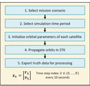
3 Simulation Approach 55 3.1 Orbit Generation & Propagation . . . 55

3.1.1 Input: Scenario Configuration . . . 57

3.1.2 Output: “Truth” State Data for All Satellites . . . 60

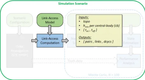
3.2.1 Input: Link-Access Model . . . 63

3.2.2 Output: Satellite Pairs, Available Links, & Duty Cycles . . . . 67

3.3 State & Measurement Simulation . . . 69

3.3.1 Input: Navigation Filter Models . . . 69

3.3.2 Output: Predicted States & Simulated Measurements . . . 73

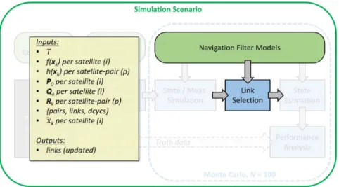
3.4 Link-Access Selection . . . 74

3.4.1 Overview of Inputs and Outputs . . . 75

3.4.2 Output: Selected Links based on CRLB . . . 75

3.5 Navigation Performance Estimation & Analysis . . . 79

3.5.1 Overview of Inputs and Outputs . . . 80

3.5.2 EKF Output: Estimation Error & Uncertainty . . . 81

3.5.3 CRLB Output: Predicted Uncertainty . . . 87

4 Earth-Orbiting Applications 89 4.1 Case Study E1: GEO Relay Satellite Systems . . . 89

4.1.1 Setup of Scenarios . . . 90

4.1.2 Single GEO-Relay with Single User . . . 93

4.1.3 Multiple Relays and/or Multiple Users . . . 101

4.2 Case Study E2: LEO Constellations . . . 106

4.2.1 Setup of Scenarios . . . 107

4.2.2 Two-satellite Navigation . . . 109

4.2.3 Walker Constellation Navigation . . . 113

4.3 Summary of Results . . . 120

4.3.1 LEO Satellites . . . 120

4.3.2 GEO Satellites . . . 120

4.3.3 HEO Satellites . . . 122

5 Deep-Space Orbital Applications 123 5.1 Case Study M1: Existing Mars Mission Orbits . . . 123

5.1.1 Setup of Scenarios . . . 125

5.1.3 Ad-hoc Constellations . . . 128

5.2 Case Study M2: Future Comms. Constellation . . . 131

5.2.1 Setup of Scenarios . . . 131

5.2.2 CRLB Uncertainty Analysis . . . 137

5.2.3 EKF Performance Results . . . 138

5.3 Summary of Results . . . 140

6 Conclusion 143 6.1 Summary of Contributions . . . 143

List of Figures

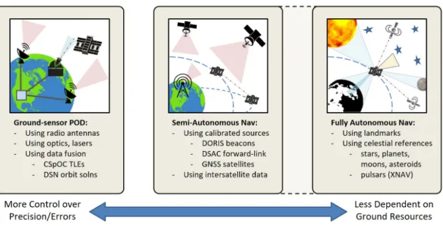
1-1 Overview of satellite navigation methods, categorized into three areas: ground-based precise orbit determination, semi-autonomous naviga-tion, and fully autonomous navigation. . . 31

1-2 Typical 1-sigma orbit estimation error achieved using ground-based tracking and autonomous navigation methods. SLR: Satellite laser ranging, VLBI: Very-long baseline interferometry, UHF: Ultra-high frequency radio ranging, NORAD (TLEs): Two-line element sets pub-lished by the North American Aerospace Defense Command, DORIS/DIODE: Doppler Orbitography and Radiopositioning Integrated by Satellite ground-beacon system and on-board OD software, DF-/SF-GNSS: Dual-/Single-frequency GNSS receivers, Landmark: Autonomous naviga-tion using landmarks, Pulsars: X-ray pulsar-based naviganaviga-tion, Inter-sat: Autonomous navigation using intersatellite measurement data, Mag-SS: Autonomous navigation using magnetometer and sun-sensors, EHS-ST: Autonomous navigation using Earth-horizon sensors and star-tracker [1–13]. . . 34

1-3 Diagram of proposed method of autonomous navigation using laser communication crosslinks between two or more satellites, co-orbital around any central-body with known gravity characteristics (mass and J2-term). This method assumes that the observing spacecraft have star-trackers for inertial attitude knowledge, and known angular off-sets between the boresights of the star tracker and the lasercom termi-nal, and other on-board systems necessary to establish and maintain a crosslink signal with another satellite. . . 39

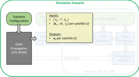
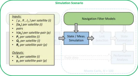
3-1 Block diagram of simulation approach: green ovals indicate inputs, blue boxes indicate written functions, and the gray box denotes external software or functions. . . 56 3-2 Results for the GEO-LEO example case: 50th percentile navigation

er-ror over 100 Monte Carlo samples of simulated lasercom crosslink mea-surements fed through an EKF intersatellite navigation filter. Results for ARTEMIS (GEO) are in black, while results for OICETS (LEO) are in red. Gray vertical bars are used to denote data-gap periods due to inaccessible crosslink geometry. . . 56 3-3 Summary of inputs and outputs for the “orbit generation and

propa-gation” step in the simulation approach. . . 57 3-4 Summary of actions taken to configure a simulation scenario. . . 58 3-5 Summary of inputs and outputs for the “link-access availability

com-putation” step in the simulation approach. . . 63 3-6 Summary of link-access constraints developed for use in this thesis. . 64 3-7 Summary of inputs and outputs for the “state and measurement

simu-lation” step in the simulation approach. . . 69 3-8 Summary of inputs and outputs for the “link-access selection” step in

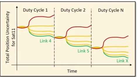
3-9 Notional diagram for the link-selection process developed for use in this thesis. Each simulation scenario is divided in time into duty-cycles, which are used as evaluation periods for link-selection. Each possible link-access partner is used in a two-satellite CRLB computation with a particular satellite (Sat11 in this case). The final CRLB value of each possible partner is compared, and the link that minimizes this value is selected. The full scenario is propagated forward using this selection, up until the start of the next duty-cycle or evaluation period. This process is repeated until the end of the simulation scenario. . . 78 3-10 Summary of inputs and outputs for the “state estimation” function in

the simulation approach. . . 80 3-11 Summary of inputs and outputs for the “performance analysis” function

in the simulation approach. . . 81 3-12 Summary of inputs and outputs for the “Monte Carlo analysis” step in

the simulation approach. . . 82 3-13 Summary of EKF results (50th percentile error averaged over final 0.5

hour) from Monte Carlo simulations (N=100) of simulation approach sensitivity to time-step, 𝑇 , in the GEO-LEO example case: a sin-gle GEO-relay satellite, ARTEMIS (black), with a sinsin-gle LEO user, OICETS (red). . . 84 3-14 Summary of EKF results (50th percentile error averaged over final 0.5

hour) from Monte Carlo simulations (N=100) of simulation approach sensitivity to initial state uncertainty, P0, in the GEO-LEO example case: a single GEO-relay satellite, ARTEMIS (black), with a single LEO user, OICETS (red). . . 84 3-15 Summary of EKF results (50th percentile error averaged over final 0.5

hour) from Monte Carlo simulations (N=100) of simulation approach sensitivity to position-estimation process noise, Qr, in the GEO-LEO example case: a single GEO-relay satellite, ARTEMIS (black), with a single LEO user, OICETS (red). . . 85

3-16 Summary of EKF results (50th percentile error averaged over final 0.5 hour) from Monte Carlo simulations (N=100) of simulation approach sensitivity to velocity-estimation process noise, Qv, in the GEO-LEO example case: a single GEO-relay satellite, ARTEMIS (black), with a single LEO user, OICETS (red). . . 85 3-17 Summary of EKF results (50th percentile error averaged over final 0.5

hour) from Monte Carlo simulations (N=100) of simulation approach sensitivity to measurement noise, R, in the GEO-LEO example case: a single GEO-relay satellite, ARTEMIS (black), with a single LEO user, OICETS (red). . . 86 4-1 Diagram of orbital scenario for the GEO Relay case study, generated

using AGI STK. . . 90 4-2 EKF results (10/50/90 percentiles) from Monte Carlo simulations (N=100)

of baseline GEO-relay example: a single GEO-relay satellite, ARTEMIS (black), with a single LEO user, OICETS (red). . . 93 4-3 CRLB analysis results for GEO satellite (ARTEMIS) with other

Earth-orbiting satellites in varying orbital altitudes and inclinations. LEO altitudes are shown in blue, lower MEO altitudes in green, GPS altitude in gray, and GEO altitude in black. Baseline GEO-LEO example of ARTEMIS & OICETS is shown in red. Lower altitude is better. . . . 95 4-4 Summary of minimum achieved CRLB over 24-hour simulation for

GEO satellite (ARTEMIS) with LEO satellites in varying orbital alti-tudes and inclinations. . . 96 4-5 CRLB analysis results for the parameter-sweep satellite (varying orbit)

in simulations of GEO satellite with other Earth-orbiting satellites in varying orbital altitudes and inclinations. LEO altitudes are shown in blue, lower MEO altitudes in green, GPS altitude in gray, and GEO al-titude in black. Baseline GEO-LEO example of ARTEMIS & OICETS is shown in red. Lower altitude is better. . . 97

4-6 Summary of minimum achieved CRLB over 24-hour simulation for the parameter-sweep satellite (varying orbit) in parameter-sweep simula-tions of GEO satellite with LEO satellites in varying orbital altitudes and inclinations. . . 98

4-7 Summary of total link-access times over 24-hour simulations of GEO "relay" satellite with LEO "user" satellites in varying orbital altitudes and inclinations. More access time is better. . . 99

4-8 EKF results (10/50/90 percentiles) from Monte Carlo simulations (N=100) of a single GEO-relay satellite, ARTEMIS (black), with a single HEO user, MMS-1 (blue). . . 100

4-9 CRLB analysis results for LEO satellite (OICETS) in different multiple-relay/user configuration: 1x GEO-relay in blue, 2x GEO-relays in or-ange, and 3x interconnected GEO-relays in yellow. Dotted curves are used for single LEO user scenarios, and solid curves for multiple users (LEO+HEO). In the legend, ‘O’ denotes those scenarios that include the LEO user OICETS, ‘M’ denotes those scenarios that include the HEO user MMS-1, and ‘G#’ denotes the number of GEO relay satel-lites used in those scenarios. . . 102

4-10 CRLB analysis results for HEO satellite (MMS-1) in different multiple-relay/user configuration: 1x GEO-relay in blue, 2x GEO-relays in or-ange, and 3x interconnected GEO-relays in yellow. Dashed curves are used for single HEO user scenarios, and solid curves for multiple users (LEO+HEO). In the legend, ‘O’ denotes those scenarios that include the LEO user OICETS, ‘M’ denotes those scenarios that include the HEO user MMS-1, and ‘G#’ denotes the number of GEO relay satel-lites used in those scenarios. . . 103

4-11 CRLB analysis results for GEO-Relay satellite #1 (at 0 deg longitude) in different multiple-relay/user configurations: 1x GEO-relay in blue, 2x GEO-relays in orange, and 3x interconnected GEO-relays in yellow. Dotted curves are used for single LEO user scenarios, dashed curves for single HEO user, and solid curves for multiple users (LEO+HEO). In the legend, ‘O’ denotes those scenarios that include the LEO user OICETS, ‘M’ denotes those scenarios that include the HEO user MMS-1, and ‘G#’ denotes the number of GEO relay satellites used in those scenarios. . . 105 4-12 EKF results (10/50/90 percentiles) from Monte Carlo simulations (N=100)

of three GEO-relay satellites equally separated in longitude (black) with a single LEO user, OICETS (red). . . 106 4-13 EKF results (10/50/90 percentiles) from Monte Carlo simulations (N=100)

of three GEO-relay satellites equally separated in longitude (black) with a single HEO user, MMS-1 (blue). . . 107 4-14 EKF results (10/50/90 percentiles) from Monte Carlo simulations (N=100)

of baseline LEO two-satellite example: TerraSAR-X (orange) with NFIRE (red). . . 109 4-15 CRLB analysis results for TerraSAR-X LEO satellite with other LEO

satellites in varying orbital altitudes and inclinations. Different al-titudes are depicted by different shades of blue: lower alal-titudes are lighter shades, and higher altitudes are darker shades. Baseline exam-ple of TerraSAR-X & NFIRE is shown in red. . . 111 4-16 Summary of minimum achieved CRLB over 24-hour simulation for

TerraSAR-X LEO satellite with other LEO satellites in varying orbital altitudes and inclinations. . . 112 4-17 Summary of minimum achieved CRLB over 24-hour simulation for the

parameter-sweep satellite (varying orbit) in parameter-sweep simula-tions of TerraSAR-X LEO satellite with other LEO satellites in varying orbital altitudes and inclinations. . . 113

4-18 Summary of total link-access times over 24-hour simulations of TerraSAR-X LEO satellite with other LEO satellites in varying orbital altitudes and inclinations. . . 114 4-19 Diagrams of orbital scenario and ground-tracks for the smallest and

largest constellations considered for a LEO Walker constellation case study, generated using AGI STK. Walker-06A denotes the Walker Delta 6/2/1 constellation, and Walker-48 denotes the Walker Delta 48/6/1 constellation. . . 115 4-20 Top: EKF results (10/50/90 percentiles) from Monte Carlo simulations

(N=100) of baseline LEO constellation example: a simple six-satellite configuration without any simultaneous links. Bottom: Depiction of which crosslink partner is available for each satellite at any given time over the course of the simulation period. . . 116 4-21 CRLB analysis results for LEO Walker Delta constellations of varying

size and distribution. The baseline Walker Delta 6/2/1 example is denoted by the thick red curve. . . 118 4-22 EKF results for LEO Walker Delta constellations of varying size and

distribution. 50th percentile results (N=100) of the baseline Walker Delta 6/2/1 example is denoted by the thick red curve. . . 119 4-23 Summary of EKF results (50th percentile over 100 Monte Carlo

sim-ulations) for LEO satellites from both the GEO-Relay and LEO Con-stellation case studies. . . 121 4-24 Summary of EKF results (50th percentile over 100 Monte Carlo

simu-lations) for GEO satellites from the GEO-Relay case study. . . 121 4-25 Summary of EKF results (50th percentile over 100 Monte Carlo

simu-lations) for HEO satellites from the GEO-Relay case study. . . 122

5-1 Diagram of orbital scenario for the Mars-orbiters case study, generated using AGI STK. . . 124

5-2 Top: Summary of EKF results (50th percentile only) from Monte Carlo simulations (N=100) of 2001 Mars Odyssey orbiter in separate two-satellite navigation scenarios with each of the other five current Mars-orbiters with a 30:30-minute communications duty cycle. Bottom: De-piction of when a link is available for each crosslink partner scenario at any given time over the course of the simulation period. . . 126

5-3 CRLB analysis results of 2001 Mars Odyssey orbiter in additive con-stellation navigation scenarios in order of launch of other five current Mars-orbiters with a 30:30-minute communications duty cycle. . . 128

5-4 Top: Summary of EKF results (50th percentile only) from Monte Carlo simulations (N=100) of 2001 Mars Odyssey orbiter in different naviga-tion scenarios with each of the other two current NASA Mars-orbiters with a 30:30-minute communications duty cycle. Bottom: Depiction of when a link is available for each crosslink partner scenario at any given time over the course of the simulation period. . . 130

5-5 Diagram of orbital scenario for the Mars communications constellation case study, based on Castellini et al. (2010) [14], generated using AGI STK. . . 132

5-6 Node diagrams depicting the topologies considered in the Mars commu-nications constellation study. “Max links/sat” describes the maximum number of simultaneous links each node can operate. “Link-Selection” shows how many of the total number of possible links in the total net-work can be used at one time, and if link-selection is active. Note that the font colors are chosen to be consistent with Figures 5-7 and 5-8. . 135

5-7 CRLB analysis results of a future 6-satellite Mars communications con-stellation [14] with a 30:30-minute communications duty cycle, and varying network topology architectures. . . 137

5-8 Summary of EKF results (50th percentile only) from Monte Carlo sim-ulations (N=100) of a future 6-satellite Mars communications constel-lation [14] with a 30:30-minute communications duty cycle, and varying network topology architectures. . . 139 5-9 Summary of EKF results (50th percentile over 100 Monte Carlo

simu-lations) for satellites from the Mars-orbiters and Mars communications constellation case studies. . . 141

List of Tables

1.1 Survey of lasercom crosslink missions. Note that the line-break in the table distinguishes past and present missions (above the line) from future missions (below). Future missions are given expected dates (in italics) based on the references cited. . . 37 2.1 Review of previous studies in autonomous navigation using

intersatel-lite measurements. Values in bold indicate those that fit the objective criteria of this thesis. . . 52 3.1 Orbital parameters for GEO-LEO example scenario. . . 59 3.2 STK settings as used to producing “truth” data for all simulations. . . 60 3.3 Central-body constants used in dynamics model, taken directly from

STK gravity model files. . . 71 3.4 Input parameters and values tested for sensitivity in simulation

ap-proach. Note that the values selected for use in this thesis are shown in bold. . . 83 3.5 Overview of case studies considered in this thesis. . . 88 4.1 Orbital parameters for GEO-Relay scenario. . . 91 4.2 Orbital parameters for simulated near-Earth orbiters in

parameter-sweep analysis, valid at time of epoch 𝑡𝑒 = 𝑡0. . . 91 4.3 Orbital parameters for simulated GEO-Relay satellites, modeled off of

the orbital parameters of EDRS-C, valid at time of epoch 𝑡𝑒 = 𝑡0. . . 92 4.4 Orbital parameters for LEO-LEO scenario. . . 108

4.5 Walker constellation configurations at 𝑎=7445.83 km, 𝑒=0, and 𝑖=60∘. 116 5.1 Orbital parameters for considered Mars-orbiter missions. Note that 𝑅

= 3,396 km for Mars. . . 125 5.2 Orbital parameters for Mars communications constellation, as

pro-posed by Castellini et al. (2010). . . 133 5.3 Network architectures used in Mars communications constellation study.134 5.4 “One-to-one” case network map, implemented as “network rules” in

Nomenclature

Symbols

𝛼 Right-ascension angle

𝛿 Declination angle

𝜆 Longitude

𝜇 Standard gravitational parameter

𝜈 True anomaly

Ω Right-ascension of the ascending node

𝜔 Argument of periapsis 𝜑 Azimuth angle 𝜌 Range, or distance 𝜎 Uncertainty/noise 𝜃 Elevation angle 𝑎 Semi-major axis 𝑒 Eccentricity ℎ Height, or altitude 𝑖 Inclination

𝐽2 Dynamic oblateness, the gravity model spherical harmonic coefficient of degree 2 and order 0

𝑀 Mean anomaly 𝑛 Mean motion 𝑅 Equatorial radius 𝑇 Duration of time 𝑡 Time Satellite Missions

ARTEMIS Advanced Relay and Technology Mission Satellite (ESA)

EDRS-A First EDRS payload (ESA), on Eutelsat-9B

EDRS-C Second EDRS payload (ESA), on dedicated satellite of same name

LADEE Lunar Atmosphere and Dust Environment Explorer (NASA)

LCRD Laser Communications Relay Demonstration (NASA), on STPSat-6

LLCD Lunar Laser Communications Demonstration (NASA)

MAVEN Mars Atmosphere and Volatile Evolution orbiter (NASA)

MEX Mars Express orbiter (ESA)

MMS Magnetospheric Multiscale (NASA)

MO 2001 Mars Odyssey orbiter (NASA)

MOM Mars Orbiter Mission (ISRO), also called “Mangalyaan” which trans-lates to “Mars-craft” in English

NFIRE Near Field Infrared Experiment satellite (DoD)

OICETS Optical Inter-orbit Communications Engineering Test Satellite (JAXA), also called “Kirari” which translates to “glitter” or “twinkle” in English STPSat-6 Space Test Program Satellite-6 (DoD)

TGO ExoMars Trace Gas Orbiter (ESA/Roscosmos)

TSX TerraSAR-X satellite (DLR)

Agencies & Organizations

AGI Analytical Graphics, Inc. (U.S. company)

CNES Centre National D’Etudes Spatiales (France), which translates to “Na-tional Center for Space Studies” in English

CSpOC Combined Space Operations Center (DoD), formerly JSpOC

DLR Deutsches Zentrum für Luft- und Raumfahrt (Germany), which

tran-lates to “German Center for Aviation and Space Flight” in English

DoD Department of Defense (U.S.A.)

ESA European Space Agency (22 member states)

ISRO Indian Space Research Organisation (India)

JAXA Japan Aerospace Exploration Agency (Japan)

JPL Jet Propulsion Laboratory (NASA)

NASA National Aeronautics and Space Administration (U.S.A.)

NGA National Geospatial-Intelligence Agency (DoD)

Roscosmos State Corporation for Space Activities (Russia)

Official Programs, Products, or Technologies

DIODE DORIS Immediate Orbit Determination (CNES)

DORIS Doppler Orbitography and Radiopositioning Integrated by Satellite (CNES)

DSAC Deep Space Atomic Clock (JPL)

DSN Deep Space Network (NASA)

DSOC Deep Space Optical Communications (NASA)

EDRS European Data Relay System (ESA)

EGM2008 2008 Earth Gravitational Model (NGA)

GNSS Global Navigation Satellite System

HORIZONS On-line solar system data and ephemeris computation service (JPL)

HPOP High-Precision Orbit Propagator (AGI)

IGS International GNSS Service

MRO110C 2012 Mars gravity model with MRO data, to degree & order 110 (JPL)

STK Systems Took Kit (AGI)

Other Abbreviations

ADC Attitude determination and control

C&DH Command and data-handling

DDOR Delta differential one-way ranging

DF Dual-frequency

DOR Differential one-way ranging

DTE Direct-to-Earth communication

EHS Earth horizon sensor

EKF Extended Kalman filter

FSOC Free-space optical communication

GEO Geosynchronous orbit

GSO Geostationary orbit

HEO Highly-elliptical orbit

ISL Intersatellite links

KF Kalman filter

Lasercom Laser communication

LEO Low Earth orbit

MEO Medium Earth orbit

OD Orbit determination

ODE Ordinary differential equation

OpNav Optical navigation

PF Particle filter

PNT Positioning, navigation, and timing

RF Radio frequency

RMSE Root-mean-square error

RTN Radial, tangential/transverse, normal reference frame

SAR Synthetic aperture radar

SF Single-frequency

SLR Satellite laser ranging

SRIF Square-root information filter

SS Sun sensor

SSO Sun-synchronous orbit

ST Star tracker

SWaP Size, weight, and power

TLE Two-line element set

TT&C Tracking, telemetry, and command

UHF Ultra-high frequency

UKF Unscented Kalman filter

UTC Primary world time standard, known as “Coordinated Universal Time" in English and “Temps Universel Coordonné” in French

VLBI Very-long baseline interferometry

Chapter 1

Introduction

1.1

Motivation

The satellite industry is undergoing a shift towards smaller and more affordable space-craft that can take advantage of reduced cost to launch [15]. This trend is ushering in new distributed satellite architectures to address critical mission areas. For example, Planet Labs Inc. has achieved unprecedented Earth imaging data with their 175+ small-satellite constellation providing global coverage and rapid revisits [16]. Beyond Earth, NASA JPL successfully demonstrated the first interplanetary CubeSats as technology demonstrators of a “carry-your-own-relay” concept, launching two MarCO spacecraft alongside the InSight Mars lander spacecraft specifically for the purpose of relaying data during InSight’s critical landing sequence back to Earth [17].

Distributed architectures, however, come with a fair share of challenges. Though satellite development and manufacturing should benefit from the economy of scale, the same cannot yet be said for ground operations. Typical satellite operations for monitoring vehicle health and status, data processing, orbit determination, task plan-ning and scheduling, and fault response are handled by teams of people per satellite. The brute-force method of handling the operations of many satellites would be build-ing more ground stations and trainbuild-ing more staff, thus resultbuild-ing in greater cost and higher risk/complexity across a global system.

de-velop higher levels of autonomy within the satellite system. Tasks typically performed by an operator and/or ground station could be shared with or fully performed by the spacecraft. Examples include planning and scheduling tasks to meet multiple objectives (e.g., maximizing data return while minimizing latency) [18], on-board data-processing to identify issues [19] or deliver data products more quickly [20], and open-loop instrument operation to obtain higher-quality data (e.g., changing sensing configurations based on geolocation or features identified in the sensor data) [8].

In order to achieve higher levels of autonomous operations, satellites should be able to precisely estimate their position and velocity states in real-time. Many ad-dress orbit determination and navigation using Global Navigation Satellite Systems (GNSS). GNSS-based navigation has become more widely used as receivers and an-tennas have become more volume- and cost-effective, as they have shown the ability to provide sub-meter positioning accuracy for low Earth orbit (LEO) objects. How-ever, achieving those small errors is highly dependent on regular or continuous receipt of ultra-rapid ephemerides and clock products from the International GNSS Service (IGS) [7]. GNSS-equipped LEO satellites more commonly achieve real-time naviga-tion solunaviga-tions on the order of 5 meters [21]. Missions in higher altitude orbits see further degraded performance as the primary service volume currently ends at 3,000 km in altitude [22].

Certain missions and applications require an alternative and enhanced autonomous navigation solution to GNSS. Military satellite applications may require redundancy in order to continue operations in potential GNSS-denied environments. Missions operating at high altitudes or orbiting other bodies (e.g., the moon or Mars) are not able to rely on GNSS-like navigation without additional relay/navigation satellite infrastructure.

The purpose of this thesis is to demonstrate an autonomous navigation method leveraging the distribution and potential connectivity of satellites in a constellation architecture to provide an alternative and enhanced navigation solution to GNSS for Earth-orbit and DSN for deep-space orbital missions. Section 1.2 provides an overview of the topics of satellite navigation methods, intersatellite links, and laser

communications in satellite systems. Section 1.3 summarizes the research objectives and contributions contained in this thesis.

1.2

Context

1.2.1

Satellite Navigation

The field of satellite navigation can be divided into two categories: (1) traditional methods of precise orbit determination (POD) using ground-sensors, and (2) au-tonomous methods using on-board sensors and navigational references. Auau-tonomous navigation can be further separated into fully-autonomous methods, which are com-pletely independent of man-made or ground-based resources, and semi-autonomous methods, which may use some external resources. Figure 1-1 summarizes the common methods in each of these categories. The following sections go into further detail on satellite navigation methods, and their relevance to this thesis.

Figure 1-1: Overview of satellite navigation methods, categorized into three areas: ground-based precise orbit determination, semi-autonomous navigation, and fully au-tonomous navigation.

Traditional Methods

Traditional methods of satellite orbit determination involve the use of ground-based sensors to track satellites and collect measurements, such as radars for range and range-rate, and telescopes for bearing angles [1, 3, 4]. This data is then processed in a filtering algorithm to estimate the six-element state of the satellite, in the form of either classical Keplerian elements such as (𝑎, 𝑒, 𝑖, Ω, 𝜔, 𝜈) or 3-dimensional position and velocity (𝑥, 𝑦, 𝑧, ˙𝑥, ˙𝑦, ˙𝑧).

The U.S. Combined Space Operations Center (CSpOC) tracks all satellites using a global network of radar and optical sensors, and publishes estimated state results in the form of two-line element sets (TLEs) for general public use. While this is useful state information for propagation forward or backward in time, performance is limited and degrades over time since the TLE epoch [23]. CSpOC’s published TLE data is also prone to errors if/when satellites are in close proximity (e.g., when multiple satellites are inserted into the same orbit around the same time) [24].

Autonomous Methods

To mitigate reliance on TLEs or building additional networks of ground sensors, several methods of autonomous navigation have been proposed and used over the last few decades. Autonomous navigation refers to satellites performing on-board, real-time navigation without external input. Such methods allow for reduced cost and risk in ground operations by eliminating the computational and logistical load of regularly tracking the satellites, estimating their individual states, and transmitting the solutions to the spacecraft [25, 26].

Fully autonomous navigation is performed without any external input, only us-ing the sensors and instruments on-board the spacecraft. Multiple techniques exist using some combination of sensors, such as cameras and infrared sensors (which can estimate state with respect to known reference points or landmarks) [13], magne-tometers (which can estimate state with respect to a known magnetic field) [12], and X-ray detectors (which can estimate state with respect to known pulsars) [10].

Semi-autonomous navigation is also performed using sensors and instruments on-board the spacecraft, but with some external input. This includes any observations made with respect to another man-made object, such as another satellite, a ground station, or a beacon. All satellite navigation using a Global Navigation Satellite System (GNSS) receiver is considered semi-autonomous, since it uses signals from a man-made source [27].

Figure 1-2 illustrates orders of magnitude of position errors demonstrated using several different techniques of precise orbit determination and autonomous navigation. Only two satellite payloads have demonstrated sub-meter real-time navigation accu-racy: GNSS receivers and DORIS/DIODE. DORIS/DIODE is a positioning method developed by the French space agency, CNES, that relies on ground beacons trans-mitting to the DORIS receiver onboard the satellite [5]. Orbit determination software specially developed to process the DORIS data (DIODE) is used to generate naviga-tion solunaviga-tions on the order of centimeters, however this has only been demonstrated for low-altitude satellites in circular orbits [28].

Since the objective of this thesis is to provide an alternative navigation method to GNSS, other methods are investigated. The fully autonomous methods shown in Figure 1-2 are only capable of providing solutions on the order of 10s-100s of meters, and utilize sensors that are heavily dependent on orbit conditions and well-characterized references. For instance, magnetometers and landmark-based sensors will likely lose sensing observability at higher altitudes; plus magnetic field models and well-characterized landmarks cannot be readily assumed for other central-bodies. The semi-autonomous navigation method using intersatellite data shows promise for use in distributed constellations. Intersatellite data refers to measurements of relative range, range-rate, or angles between two spacecraft. Previous work has found the intersatellite autonomous navigation method to be accurate on the order of 10s of meters [9, 11], which is better than the fully autonomous methods and resembles the performance of single-frequency GNSS receivers, though results have not yet been experimentally demonstrated on-orbit. Still, the promise of the intersatellite method to this thesis is realized in its independence of the orbit configuration of either satellite,

Figure 1-2: Typical 1-sigma orbit estimation error achieved using ground-based tracking and autonomous navigation methods. SLR: Satellite laser ranging, VLBI: Very-long baseline interferometry, UHF: Ultra-high frequency radio ranging, NORAD (TLEs): Two-line element sets published by the North American Aerospace Defense Command, DORIS/DIODE: Doppler Orbitography and Radiopositioning Integrated by Satellite ground-beacon system and on-board OD software, DF-/SF-GNSS: Dual-/Single-frequency GNSS receivers, Landmark: Autonomous navigation using land-marks, Pulsars: X-ray pulsar-based navigation, Intersat: Autonomous navigation using intersatellite measurement data, Mag-SS: Autonomous navigation using mag-netometer and sun-sensors, EHS-ST: Autonomous navigation using Earth-horizon sensors and star-tracker [1–13].

and thus its ability to leverage greater separations between satellites, such as in a constellation. Assuming intersatellite range and angle measurements are available, this method is viable for satellites in distributed orbits, and could even perform better when used in a constellation.

Current State-of-the-Art

For near-Earth orbiting satellites, Global Navigation Satellite Systems represent the current state-of-the-art for spacecraft navigation, primarily for its capability as an autonomous method, its availability in different orbital regime, and most importantly, its performance. Recent literature has shown that GNSS receivers are capable of

achieving solution errors on the order of 3-5 meters in low Earth orbit (LEO) [21]. A few missions have also been used to test GNSS receivers at altitudes greater than the constellation altitude, and have admirably shown solution errors on the order of 12-15 meters in geosynchronous orbit (GEO) [29], and 25-65 meters in highly eccentric orbit (HEO) [22].

For deep-space applications, the Deep Space Network of tracking stations rep-resents the current state-of-the-art for spacecraft navigation, capable of navigation accuracy (for Mars-orbiters) down to 25 meters during periods of DSN downlink, and 100 meters during periods without downlink [30].

These navigation performance values are used to generate performance targets for the intersatellite navigation method using lasercom crosslinks. In each case, we set a threshold to which we will compare the results of different orbital scenarios in this thesis. These are 3 meters for LEO, 12 meters in GEO, 45 meters in HEO, and 25 meters in Mars-orbit.

1.2.2

Crosslink Communications

Intersatellite measurements may easily be made if the constellation is designed for crosslink communications, also known as intersatellite links (ISLs). One benefit of implementing crosslinks in a satellite system is increasing ground access for space-craft tracking, telemetry, and command (TT&C) operations without needing to add more ground stations. For communications and Earth-observing missions, crosslinks can also serve to increase data-to-ground by mitigating downlink bottlenecks and re-ducing latency between terminals [18, 31]. For Positioning, Navigation, and Timing (PNT) missions, crosslinks are used to improve the quality of the PNT information, increase system reliability and robustness, and enhance availability to higher alti-tude orbits [32, 33]. In addition to intersatellite measurements, crosslinks also enable other new capabilities in satellite systems, such as distributed processing, and new methods of navigation or formation-control by communicating measurements or state estimates between vehicles [34]. A number of previous studies make the assumption that intersatellite links exist in future constellation systems, and can be leveraged for

autonomous navigation. A more detailed review of previous work can be found in Section 2.2. This thesis also assumes the existence of crosslinks for use in autonomous navigation.

Lasercom Links

Lasercom provides improved energy efficiency, data rates, latency, and security com-pared with traditional radio-frequency (RF) communications systems [35]. Muri and McNair (2012) performed a survey of all intersatellite link demonstrations until 2012 as well as those that were expected to launch through 2015 [31]. Since the time of Muri and McNair (2012), there has been an notable uptick in the number of launched and proposed missions to utilize optical ISLs, as shown in Table 1.1. Recent years have seen multiple European Data Relay Satellite (EDRS) systems launched into GEO for the purpose of quickly and efficiently relaying critical Earth-observation data from ESA’s Copernicus/Sentinel satellites to ground [36]. The upcoming slate includes similar relay technology demonstrators from JAXA, NASA, and Airbus.

T able 1.1: Surv ey of lasercom crosslink missions. Note that the line-break in the table di stinguishes past and presen t missi o n s (ab o v e the line) from futu re missions (b elo w). F uture missions are giv en exp ecte d dates (in italics) based on the references cited. Y ear [ref ] Platforms En vironmen t Mission 2001 [31] SPOT-4 – AR TEMIS LEO–GEO T ec hnology Demo. (1st one-w a y link) 2005 [31] OICETS – AR TEMIS LEO–GEO T ec hnology Demo. (1st tw o-w a y link) 2008 [31] T erraSAR-X – NFIRE LEO–LEO T ec hnology Demo. (1st LEO-LEO link) 2014 [37] Sen tinel-1A – Alphasat LEO–GEO GEO Rela y T ec hnology Demo. [ESA] 2016-presen t [36] Sen tinel (x4) – EDRS (x2) LEO–GEO Op erational GE O Rela y System [ESA] 2019 [38] A eroCub e-7B – ISARA LEO–LEO Cub eSat P oin ting Demo. [A erosp a ce Corp.] 2020 [39] ILLUMA-T (ISS) – LCRD LEO–GEO GEO Rela y T ec hnology Demo. [NASA] 2020 [40] ALOS-4 – JDRS LEO–GEO GEO Rela y T ec hnology Demo. [JAXA] 2020 [41] SpaceX “Starlink” Constellation LEO–LEO (W alk er) Global Broadband Comm un ica ti o n s 2021 [42] CLICK-B – CLI CK -C LEO–LEO Cub eSat P a yload Demo. [MIT, UF] 2021 [43] Cloud Constellation “SpaceBelt” LEO–LEO (Ring) Global Data Securit y 2022 [44] T eleSat LEO Constellation LEO–LEO (W alk er) Global Broadband Comm un ica ti o n s 2022 [45] Laser Ligh t Comms. “HALO” MEO–MEO (Ring) Global Net w ork Comm unications Service 2023 [39] Gen-2 GEO Rela y LEO–GEO(–GEO) Op erational GE O Rela y System [NASA]

McCandless and Martin-Mur (2016) also investigated a future DSN-like network using optical communications systems and performed simulations to compare position accuracy with the current capability of DSN radiometric tracking for a future Mars lander and Mars orbiter. The authors concluded that optical tracking stations could feasibly be an improvement over the current radiometric capability [30].

This thesis builds on the notion of using lasercom systems for crosslinks in order to collect intersatellite data measurements for autonomous navigation.

1.3

Thesis Overview

In order to measure intersatellite range and bearing between satellites in a constel-lation, we propose using lasercom crosslinks, expanding on the concept studied by Yong et al. (1983) [46]. Figure 1-3 provides a depiction of our proposed method.

Time-of-flight ranging measurements can be captured using time-embedded sig-nals over communications links [47]. Laser communications payloads operate at op-tical wavelengths with greater frequency bandwidth than RF systems. The higher bandwidth enables lasercom systems to measure range between two terminals with more precision. RF systems typically achieve meter-level ranging precision [48]. Lasercom systems can achieve centimeter-level precision; the current state-of-the-art performance in satellite lasercom ranging was demonstrated to about 1-cm precision in two-way links from Earth to lunar orbit during the Lunar Laser Communication Demonstration (LLCD) mission in 2015 [49]. However, this was a ground-to-satellite demonstration, not satellite-to-satellite.

When compared to RF systems, intersatellite lasercom systems have narrow beamwidths, typically less than 1 degree [42]. In order to point the narrow beam signal directly at the receiving terminal, lasercom demands highly accurate pointing systems, which can be leveraged to obtain the bearing between the two satellites. Assuming a lasercom crosslink can be established between two satellites, we propose deriving intersatellite bearing by determining the body attitude of the spacecraft using an on-board star tracker, using any angular offsets between boresights of the lasercom transceiver and

Figure 1-3: Diagram of proposed method of autonomous navigation using laser com-munication crosslinks between two or more satellites, co-orbital around any central-body with known gravity characteristics (mass and J2-term). This method assumes that the observing spacecraft have star-trackers for inertial attitude knowledge, and known angular offsets between the boresights of the star tracker and the lasercom terminal, and other on-board systems necessary to establish and maintain a crosslink signal with another satellite.

star tracker. If the lasercom payload is fixed to the spacecraft body, these offsets are fixed values that are either known from the design of the spacecraft, or defined using an on-board calibration process. If the lasercom payload is on a gimbal, then commanded offsets must also be included in order to fully capture angular offsets between the boresights of the payload and star tracker.

Long-range RF crosslinks typically cannot be used to similarly derive bearing to the receiving satellite due to the relatively large beamwidth of RF systems. For instance, GNSS satellite antenna half-beamwidths are on the order of 23-26 degrees [50]. In order to measure intersatellite bearing, additional sensors must also be used, such as telescopes or camera/beacon systems. Passive electro-optical sensors are

limited by observability constraints that effectively limit the separation between the two satellites in which bearing can be measured. For example, cameras are affected by apparent magnitude and proper illumination of the other spacecraft [48], and can only work for separations of a few hundreds of kilometers between satellites. Active sensors, such as beacon systems, can be used for longer ranges [51, 52]. Lasercom crosslinks can be considered a form of an active electro-optical system, capable of working over longer ranges [38, 42].

For this study, we assume that all satellites have at least one lasercom termi-nal, with parameters consistent with those offered by commercial companies [53] or currently being developed [42], along with the accompanying subsystems for power, attitude determination and control (ADC), and command & data handling (C&DH). These systems must operate together in order to establish and maintain a lasercom crosslink between two communicating spacecraft. We assume that crosslinks are es-tablished using methods such as performing a scanning maneuver or implementing a coarse beacon system [42].

1.3.1

Research Contributions

The three contributions in this thesis are:

∙ Creation of a simulation framework to estimate the performance of autonomous navigation methods using intersatellite measurements for varying orbital envi-ronments, satellite constellations, sensor network configurations, and measure-ment models. This includes a kinematic uncertainty approximation algorithm using Cramér Rao lower bound (CRLB) covariance estimates as a link selection heuristic when multiple links are available.

∙ Analysis of the navigation performance over relevant past, present, and future crosslinked satellite missions to demonstrate the method’s applicability to both near Earth and deep space environments, including assessment of lasercom in-terconnectivity on constellation navigation.

∙ Demonstration of improved navigation performance using autonomous laser-com crosslinks over current spacecraft navigation techniques (GNSS for Earth orbiters, DSN for deep space) with median total position errors (from Monte Carlo simulations) better than 3 meters for LEO, 12 meters for GEO, 45 meters for HEO, and 25 meters for Mars orbiters.

1.3.2

Organization

Chapter 2 contains background in spacecraft navigation and a review of previous literature in the area of intersatellite navigation with the goal of identifying research gaps to be addressed by the work in this thesis. Chapter 3 describes the simulation approach, and Chapters 4 and 5 present the results of simulations in Earth-orbiting and Mars-orbiting applications, respectively. Chapter 6 summarizes the contributions and conclusions made in this thesis.

Chapter 2

Background & Literature Review

This chapter provides a high-level review of traditional spacecraft navigation esti-mators and measurements, then performs a deeper analysis of previous work in au-tonomous navigation using intersatellite measurements in order to identify research gaps and highlight relevant insights towards achieving the objectives of this thesis.

2.1

Spacecraft Navigation Methodology

Spacecraft navigation estimation relies on using a time-series of measurements to estimate observables that are directly influenced by the gravitational forces existing in the space environment. This section describes commonly used estimation methods and measurements for spacecraft navigation.

2.1.1

Estimation Methods

State estimation can either be done by considering measurements all-at-once (a batch process) or as each measurement is made (a sequential process). Batch processes rep-resent the traditional methods for determining post-processed orbit solutions. Sequen-tial processes represent filtering methods that can be used for real-time navigation solutions.

Batch Least-Squares Processing

Least-squares estimation is a commonly used method for approximating the values of unknown parameters that best-fit the input data based on an expected model of behavior. The term “least-squares” refers to the objective of minimizing the sum of the square of the difference between an observed value and an expected value based on the model. This is captured by the following equation:

^

x = (H𝑇H)−1H𝑇y (2.1)

where ^x is the estimated state, and H is the measurement model that describes the relationship between the state vector, x, and the measurements, y. For a nonlinear, differentiable measurement model function ℎ(x) and measurement noise v:

y = ℎ(x) + v (2.2)

the following Jacobian can be calculated to linearize the model at each measurement time-step:

H = 𝜕ℎ

𝜕x (2.3)

Sequential Kalman Filtering

The Kalman Filter (KF) is an optimal estimator for linear Gaussian systems. As a method of sequential processing, it is commonly used for real-time navigation solu-tions. The filter is divided into two phases, the prediction phase, which propagates the most recent state estimate and covariance to the current time-step, and the up-date phase, which uses any available measurements at the current time-step to upup-date the predicted state estimate and covariance.

The dynamics model (or state-transition model) F𝑘 is described by:

x𝑘 = F𝑘x𝑘−1+ w𝑘 (2.4)

and w𝑘 is the process noise with normal distribution and covariance Q𝑘. The measurement model is described by:

y𝑘= H𝑘x𝑘+ v𝑘 (2.5)

where y𝑘 are the measurements observed at each filter step 𝑘 ∈ {1, · · · , 𝑁 }, and v𝑘 is the measurement noise with normal distribution and covariance R𝑘.

The prediction phase is:

^

x𝑘|𝑘−1= F𝑘x^𝑘−1 (2.6)

P𝑘|𝑘−1 = F𝑘P𝑘−1F𝑇𝑘 + Q𝑘 (2.7)

where x0 and P0 reflect the a priori knowledge of the initial state and covariance values.

The update phase is:

^

x𝑘 = ^x𝑘|𝑘−1+ K𝑘[y𝑘− H𝑘x^𝑘|𝑘−1] (2.8)

P𝑘 = (I − K𝑘H𝑘)P𝑘|𝑘−1 (2.9)

where K𝑘 is the Kalman gain:

K𝑘 = P𝑘|𝑘−1H𝑇𝑘(H𝑘P𝑘|𝑘−1H𝑇𝑘 + R𝑘)−1 (2.10)

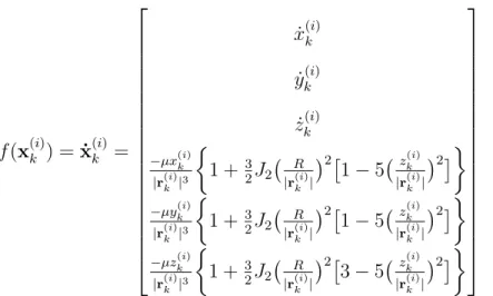
The Extended Kalman Filter (EKF) performs the same computations as the Kalman Filter except that the dynamics and measurement models may be nonlin-ear, differentiable functions, 𝑓 (x) and ℎ(x), respectively:

x𝑘 = 𝑓 (x𝑘−1) + w𝑘 (2.11)

y𝑘= ℎ(x𝑘) + v𝑘 (2.12)

Jacobian matrices, F𝑘 and H𝑘, are computed matrices for use in the prediction and update phases:

F𝑘= 𝜕𝑓 𝜕x ⃒ ⃒ ⃒ ⃒ ^ x𝑘−1 (2.13) H𝑘= 𝜕ℎ 𝜕x ⃒ ⃒ ⃒ ⃒ ^ x𝑘|𝑘−1 (2.14)

The use of Jacobians linearizes the nonlinear functions around the most recent es-timate, which is effective for low-order nonlinearity, but can be problematic for highly nonlinear functions for which Jacobian matrices cannot be easily derived (analytically or numerically). For these types of problems, the Unscented Kalman Filter (UKF) can be used. The UKF avoids linearization via Jacobians by computing mean and covariance estimates using a set of deterministic sample points (called sigma points) propagated through the nonlinear functions 𝑓 (x) and/or ℎ(x).

Kalman filters and its variants are commonly used for navigation problems, but are known to exhibit initialization and numerical stability issues. Applications that may be affected by such effects often implement a Square-Root Information Filter (SRIF) instead, which propagates the square-root of a state information matrix in-stead of a state-transition matrix that requires matrix inversions, leading to more robust numerical stability and the ability to handle high initial variance. Another common estimator is the Particle Filter (PF), which uses probability density func-tions to randomly generate sample points to model nonlinear dynamical systems. This is similar to the UKF, although PF methods tend to use a higher quantity of sample points. Thus PF methods have seen more use recently as computation and processing have become faster and cheaper. Only the EKF is used in this thesis, but other filters like SRIF and PF can be implemented in future work.

Cramér-Rao Lower Bound (CRLB)

The Cramér-Rao lower bound computes the lowest achievable covariance or expected errors assuming optimal filter performance. It is commonly used to evaluate state estimator precision and observability [48, 54–56]. Relevant to the context of this thesis, it can also be used to predict covariance for “efficient” estimators, those that

achieve the CRLB, such as the extended Kalman filter [54]. The CRLB is defined by the following equations:

P𝑘 ≥ J−1_𝑘 (2.15) where J𝑘 = (¯F𝑘−1J−1𝑘−1F¯ 𝑇 𝑘−1+ Q𝑘)−1+ ¯H𝑇𝑘R −1 𝑘 H¯𝑘 , J0 = P−10 (2.16)

2.1.2

Measurement Types

This section presents background framework on common measurements made for spacecraft navigation. For each measurement type, we describe how the measure-ments are derived, and list a couple example systems that collect that type of mea-surement.

Range

Range is the measurement of distance or relative position between two points:

𝜌(𝑖𝑗) = |Δr(𝑖𝑗)| (2.17)

where Δr(𝑖𝑗) = r(𝑗) _{− r}(𝑖) _{is the relative position vector between points 𝑖 and} 𝑗. In terms of spacecraft navigation, point 𝑖 describes the Cartesian position of the observer, and point 𝑗 describes the Cartesian position of the observed satellite. The observer may be a ground-based or space-based sensor.

Range is typically derived by measuring the one-way or two-way time-of-flight, 𝑡, of an electromagnetic signal between the two points. Since the signal travels at the speed of light, 𝑐, the distance traveled by the signal can be determined by the kinematic equation 𝑑 = 𝑐×𝑡, assuming any sources of error are calibrated out, and any ambiguities are resolved using estimation algorithms. In two-way methods, 𝜌 = 𝑑/2. This technique is commonly used by radar and laser sensors, such as those in Deep Space Network and Satellite Laser Ranging tracking stations.

Range can also be derived via signal intensity. One example of this technique is in optical astrometry, in which the size of an observed target on its sensor plane is mapped to a specific range value via a well-characterized and calibrated function of size versus range. This is commonly used for optical autonomous navigation (OpNav).

Range-Rate

Range-rate is the rate-of-change in the distance or relative position between two points:

˙

𝜌(𝑖𝑗) = Δr

(𝑖𝑗)_{· Δ˙r}(𝑖𝑗)

|Δr(𝑖𝑗)| (2.18)

where Δ˙r(𝑖𝑗) = ˙r(𝑗) _{− ˙r}(𝑖) _{is the relative velocity vector between points 𝑖 and} 𝑗. In terms of spacecraft navigation, point 𝑖 describes the Cartesian position of the observer, and point 𝑗 describes the Cartesian position of the observed satellite. The observer may be a ground-based or space-based sensor.

Range-rate is typically obtained by measuring the Doppler frequency shift, 𝑓𝑑, of an electromagnetic signal received or returned by the observed target. This relation-ship is described by the equation:

˙

𝜌 = 𝜆𝑓𝑑

2 (2.19)

where 𝜆 is the wavelength of the transmit signal. This technique is commonly used by radar sensors like DSN antennas, and beacon systems like the DORIS receiver.

Bearing (Angles)

A bearing measurement is the angle between a reference direction and the position of an object, in this case the observed satellite target. For spacecraft navigation, two bearing angles (𝜑 and 𝜃) are typically used to fully describe the relative direction to a target, either Azimuth and Elevation, or Right Ascension and Declination (which are equivalent angles in different reference frames):

𝜑(𝑖𝑗) = arctan(︂ ∆𝑦 (𝑖𝑗) ∆𝑥(𝑖𝑗) )︂ , from 0 to 2𝜋 (2.20) 𝜃(𝑖𝑗) = − arcsin(︂ ∆𝑧 (𝑖𝑗) |Δr(𝑖𝑗)_| )︂ (2.21) where ∆𝑥(𝑖𝑗) = 𝑥(𝑗)− 𝑥(𝑖) _{, ∆𝑦}(𝑖𝑗) _{= 𝑦}(𝑗)_{− 𝑦}(𝑖) _{, ∆𝑧}(𝑖𝑗)_{= 𝑧}(𝑗)_{− 𝑧}(𝑖) _(2.22)

Bearing angles can be derived from measuring mechanical displacement (i.e., the angular displacement of a telescope mount or a gimbaled platform in mechanically-pointed sensors), measuring relative signal delays at known positions (e.g., the method used in very-long baseline interferometry, or VLBI), or via astrometry (i.e., determin-ing the attitude of a sensor image relative to the directions of known, fixed objects in the image like stars).

2.2

Autonomous Navigation with Intersatellite Data

2.2.1

Seminal Research

The first study of using intersatellite range and inertially-referenced bearing measure-ments for determining the orbits of two satellites without any a priori information was conducted by F.L. Markley and published in 1984. The author first performed an observability analysis to determine the feasibility of such a method. Using a simple spherical Earth gravity model, Markley concluded that a few certain orbit cases are unobservable using this method: when both spacecraft have equal semi-major axis 𝑎, equal eccentricity 𝑒, equal “phasing” (i.e., mean-anomaly, 𝜈), and are either coplanar, or “oriented so that the two spacecraft cross the line of intersection of the two planes simultaneously” when non-coplanar [9].

These findings were furthered in a study by M.L. Psiaki in 1999, using a higher-fidelity Earth gravitational model with 𝐽2 secular perturbations. This study

con-cluded that only one orbit case is absolutely unobservable: the same case as described earlier (when both spacecraft have equal 𝑎, equal 𝑒, and equal 𝜈), but specifically when the satellites are coplanar at the inclination 𝑖 of 0∘ . This means that inclined and non-coplanar orbit cases are semi-observable due to the non-spherical Earth, and that errors would grow as the two-spacecraft system more closely resembles the absolute unobservable case. This conclusion largely affects satellites in GEO observing each other, as they are all in low-inclination circular orbits. Missions in other orbits can be affected too, though satellites in LEO and MEO tend to be inclined. We would also like to note that the absolute unobservable case can still be mitigated by observing satellites at other altitudes, such as between GEO and LEO. This is of particular interest for study in this thesis.

Psiaki also established some baseline performance references by reporting posi-tion uncertainty as a funcposi-tion of altering intersatellite geometry between two Earth-orbiting satellites. This analysis showed observability errors caused by small sepa-rations between satellites (on the order of 100 km), lack of measurement variability in specific state elements, proximity to the absolute unobservable case, orbital alti-tude, and high angle measurement uncertainty [11]. We intend to report on similar effects but in an expanded range of potential orbital geometries afforded by the longer separations possible using lasercom links.

In this thesis, while the source of the measurement is different from those used in the aforementioned observability analyses (RF systems vs. lasercom systems), the measurement types (range and bearing) have not changed; therefore an observability analysis is not repeated in this work. However, we are interested in evaluating the effect of estimation observability on navigation performance. As mentioned Section 2.1.1, one way to evaluate the effect of observability on error performance is to com-pute the CRLB. Thus, CRLB computations are an important part of our analyses.

2.2.2

Other Relevant Studies & Analyses

Table 2.1 shows a summary of previous work in autonomous navigation using inter-satellite measurements. In reviewing this area of research, we report a few

differenti-ating characteristics of each study that are of particular interest to this thesis. These include the quantity and distribution of satellites and the uncertainty values of the measurements, all as modeled and used in each study’s respective simulations. In the final column, we report the magnitude of the resulting navigation performance of each study.

Of the 17 studies reviewed, five studies simulate constellations larger than 4 satel-lites, five studies simulate intersatellite geometry with separations on the order of tens of thousands of kilometers, six studies model ranging precision below 1 meter, and six studies model angular precision below 5 arcsec. However, only four studies possessed two or more of these characteristics, while only one possessed all, Gao et al. (2014).

Psiaki (1999) modeled precise range and bearing measurements for largely sep-arated satellites, but only for two-satellite Earth-orbiting systems [11]. Zhao et al. (2011) simulated a 30-satellite constellation comprised of distributed satellites in both LEO and GEO using a neutral value of ranging precision, but did not model any bearing measurements (possibly due to the large separations between satellites) [61]. Li et al. (2017) simulates a 6-satellite constellation with very precise bearing mea-surements, but a strangely high uncertainty in ranging [68]. This study also does not provide any details regarding the orbital configuration of the constellation, and therefore the actual modeled distribution of satellites is unknown.

Gao et al. (2014) was the only study to possess all of the characteristics of interest in this thesis [63]. In this study, the authors propose a navigation constellation com-prised of 12 GNSS satellites in MEO and 4 satellites in Earth-Moon Lagrangian point orbits (LPO). Three cases are considered: (1) only GNSS satellites with only ranging measurements, (2) only GNSS satellites with range and angle measurements, and (3) GNSS + LPO satellites with only ranging measurements. The authors conclude that while range and angle measurements (case 2) show improved precision and stability over case 1, ranging with satellites in Lagrangian points demonstrates even better performance. Position errors were reported on the order to tens of meters. Case 2 is of most immediate relevance to this thesis, however no details are given regarding