Autonomous aerobatic maneuvering of miniature helicopters

(1)

Autonomous Aerobatic Maneuvering of Miniature

Helicopters

by

Vladislav Gavrilets

Submitted to the Department of Aeronautics and Astronautics in partial fulfillment of the requirements for the degree of

Doctor of Philosophy at the

MASSACHUSETTS INSTITUTE OF TECHNOLOGY

May 2003

MASSACHUSETTS INSTITUTE OF TECHNOLOGY

SEP 1 0 2003

LIBRARIES

@

Author...

Certified by...

...

Dep ment of Aeronautics and Astronautics

May 2, 2003

...

Eric Fei on Associate Professor of Aeronautics and Astronautics Thesis Supervisor

Munther Dahleh Profes pf Electrical Engineering 'S' S ervisor

...

David Vos Chief Technology Officer, Athena Technologies Thesis Supervisor Certified by...

V fCarlos Uesnik

Associate Professor of Aerospace Engineering, University of Michigan Thesis Supervisor Accepted by...

Edward Greitzer Slater Professor of Aeronautics and Astronautics Chairman, Department Committee on Graduate Students

(2)

(3)

Autonomous Aerobatic Maneuvering of Miniature Helicopters by

Vladislav Gavrilets

Submitted to the Department of Aeronautics and Astronautics on May 2, 2003, in partial fulfillment of the

requirements for the degree of Doctor of Philosophy Abstract

In this thesis, I present an experimentally proven control methodology for the autonomous execution of aerobatic maneuvers with small-scale helicopters, and a low-order dynamic model which adequately describes a miniature helicopter in a wide range of flight conditions, including aerobatics. The control laws consist of steady-state trim trajectory controllers, used prior to, and upon exit from the maneuvers; and a maneuver execution logic inspired by human pilot strategies. In order to test the control laws, a miniature helicopter was outfitted with a custom digital avionics system, and a hardware-in-the-loop simulation was developed. The logic was tested with several aerobatic maneuvers and maneuver sequences, which demonstrated smooth maneuver entry, automatic recovery to a steady-state trim trajectory, and robustness of the trim-trajectory control system toward measurement and modeling errors. Based on these results, I further propose a simplified hybrid model for a helicopter under such closed loop control. The model can be utilized in the development of computationally tractable motion-planning algorithms for agile vehicles.

Thesis Supervisor: Eric Feron

Title: Associate Professor of Aeronautics and Astronautics Thesis Supervisor: Munther Dahleh

Title: Professor of Electrical Engineering Thesis Supervisor: David Vos

Title: Chief Technology Officer, Athena Technologies Thesis Supervisor: Carlos Cesnik

(4)

(5)

Acknowledgments

First of all, I would like to thank my advisors Eric Feron and David Vos for their constant support, and infinitely many insights, technical and beyond, they gave me over the years.

I am happy to credit Eric with the idea that started this thesis: to demonstrate that aerobatic maneuvers can be performed fully autonomously by an aerial robot, in a manner similar to the way human pilots perform them. Eric has been an incredibly enthusiastic supporter, and at the same time steered the course of the project with great wisdom. I have greatly enjoyed our many irreverent conversations; his house, full of kids, was always warm with hospitality.

Dave Vos largely shaped me as an engineer while I worked under his guidance at Aurora Flight Sciences, and later, when he generously agreed to volunteer his precious time to advise me in the Ph.D. program. I can not overestimate the value of his expert advice throughout the course of the project. His ability to see through seemingly complicated engineering problems is truly unique. One winter day I spent at Dave's house on Cape Cod, discussing approaches to modeling and control of aerobatic helicopters, gave me the roadmap for the rest of the project.

I was lucky to have a chance to interact with Prof. Munther Dahleh, who served on my thesis committee. Munther is a great teacher, being his teaching assistant in the class on dynamic systems was intellectually stimulating, and truly enjoyable.

Prof. John Hansman has kindly provided technical advice in the design of helicopter ground station display, and offered useful critical feedback for this manuscipt.

Prof. Carlos Cesnik, currently of University of Michigan, gave an excellent introduction to structures in his class, and effectively steered my program of studies in this area.

During both my Master's and Ph.D. program I got invaluable knowledge and inspiration from M.I.T. faculty. I am happy to acknowledge professors John Deyst, Dave Trumper, Jim Paduano, Mark Drela, Sanjoy Mitter, Dimitri Bertsekas, Marthinus Van Schoor and Klaus-Jurgen Bathe, for providing me with world-class education and making the process of acquiring it enjoyable.

I would like to thank Dr. Bernard Mettler, my colleague at M.I.T. and frequent co-author, for sharing his expertise in helicopter dynamics and his infinite patience in teaching me a proper style of technical writing.

I would like to acknowledge Prof. Emilio Frazzoli, currently of University of Illinois at Urbana-Champaign, who provided many insights during our discussions while he was a student at M.I.T. and afterwards.

This work would be impossible without the contributions of several M.I.T. students who worked with me on this hard project. I am very thankful to Ioannis Martinos, Kara Sprague, Alex Shterenberg, Rodin Lyasoff, David Dugail, and Allen Wu for contributing countless hours, frequently during week-ends and well into the nights.

My experience at M.I.T. was especially enjoyable thanks to many other interesting people, among them LIDS students Jan DeMot, Masha Ishutkina and Tom Schovenaars.

I owe infinite gratitude to my family, especially to my mother Elizaveta and my sister Evgenia, for their unconditional love and support.

(6)

(7)

3.1 Overview of Modeling Approaches . . . . 3.2 Helicopter parameters . . . . 3.3 Equations of motion . . . . 3.4 Component forces and moments . . . . 3.4.1 Main rotor forces and moments . . . . 3.4.2 Engine, governor and rotorspeed model . . . . . 3.4.3 Fuselage forces . . . . 3.4.4 Vertical fin forces and moments . . . . 3.4.5 Horizontal stabilizer forces and moments . . . . . 3.4.6 Tail rotor . . . . 3.5 Actuator models . . . . 3.6 Sensor m odels . . . . 3.6.1 Inertial measurement unit . . . . 3.6.2 Global Positioning System Receiver . . . . 3.6.3 Barometric altimeter . . . . 4 Control system design for autonomous aggressive

4.1 Control approach and autopilot modes . . . . 4.2 Longitudinal-vertical trim trajectory controller

4.2.1 Linearized longitudinal-vertical dynamics 4.2.2 Model reduction for control system design 4.2.3 Control system design . . . . 4.3 Lateral-directional trim trajectory controller . . . . 4.3.1 Linear model and control design . . . . 4.4 Human-inspired logic for automatic maneuvering .

mane ivering 55 . . . . 55 . . . . 61 . . . . 61 . . . . 62 . . . . 62 . . . . 65 . . . . 66 . . . . 69

4.4.1 Axial roll maneuver . . . . 13 13 16 17 . . . . 1 7 . . . . 1 9 . . . . 22 . . . . 28 31 . . . . 3 1 . . . . 3 2 . . . . 33 . . . . 3 3 . . . . 33 . . . . 44 . . . . 46 . . . . 47 . . . . 48 . . . . 48 . . . . 5 2 . . . . 52 . . . . 5 2 . . . . 54 . . . . 54 70

(8)

4.4.2 Split-S maneuver . . . . 71 4.4.3 Autonomous airshow routine . . . . 72 4.5 Simplified hybrid model for motion planning . . . . 73

5 Conclusions and future work 79

5.1 Summary . . . . 79 5.2 Future research . . . . 81

(9)

List of Figures

1-1 Miniature helicopter undergoing a Split-S maneuver. The same maneuver was performed fully autonomously using the control methods developed in

this thesis. Drawing courtesy of Popular Mechanics magazine. . . . . 14

2-1 Instrumented X-Cell helicopter in flight . . . . 18

2-2 Transmissibility function for different materials . . . . 19

2-3 Vibration-isolated avionics assembly . . . . 20

2-4 Hardware-in-the-loop simulation . . . . 28

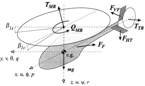
3-1 Moments and forces acting on helicopter . . . . 35

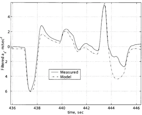
3-2 Modeling vertical acceleration response at hover . . . . 38

3-3 _{Rotor moments acting on the helicopter fuselage . . . .} ₄₀

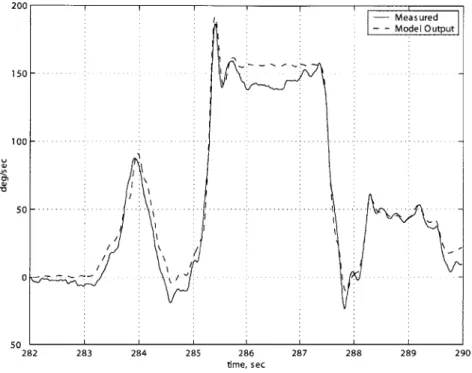
3-4 _{Actual and model roll rate response during axial roll maneuver . . . .} ₄₂

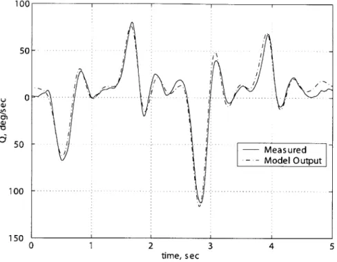
3-5 _{Actual and model pitch rate response in low-speed flight . . . .} ₄₃

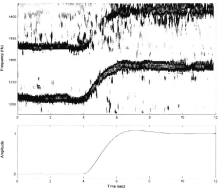
3-6 (top) Two frequency bands in the engine noise spectrum; (bottom) Simulated response to rotorspeed step command . . . . 46

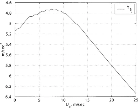
3-7 Linearized tail rotor sideforce due to side velocity . . . . 50

3-8 Linearized tail rotor sideforce due to tail rotor pitch . . . . 50

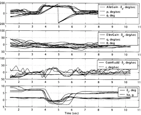
4-1 Recorded state and input time histories for multiple axial roll maneuvers. The variables of interest are the pilot lateral cyclic control (6a), the helicopter roll angle (#), and the pilot collective controll (coll) . . . . 57

4-2 Recorded state trajectory during a manual axial roll . . . . 58

4-3 Recorded state trajectory during an axial roll with rate tracking controllers 59 4-4 Comparing pilot rate command with a piece-wise linear approximation . . . 60

4-5 _{Longitudinal cyclic to pitch rate transfer function approximations . . . .} ₆₃

4-6 _{Longitudinal-vertical control architecture . . . .} ₆₄

4-7 Forward velocity and altitude time histories during rapid acceleration and deceleration . . . . 65

4-8 Lateral-directional controller structure . . . . 66

4-9 Lateral-directional gain variation with forward speed . . . . 67

4-10 Bank angle response . . . . 68

4-11 Phases of an autonomous aerobatic maneuver . . . . 69

4-12 Reference roll rate trajectory for axial roll maneuver . . . . 70

4-13 Recorded state trajectory during an autonomous axial roll . . . . 71

4-14 Pitch and roll rate reference trajectories for split-S maneuver . . . . 72

4-15 Recorded state trajectory during an autonomous split-S . . . . 73

(10)

4-17 A state machine for the autonomous airshow routine . . . . 75

4-18 Flight data for the autonomous split-S -hammerhead sequence . . . . 76

4-19 A state machine representation of helicopter behavior. Dashed lines are used to indicate that certain transitions may not be allowed depending on vehicle state ... ... 76

4-20 First-order approximation of the closed-loop velocity response . . . . 77

4-21 First-order approximation of the closed-loop yaw rate response . . . . 77

(11)

List of Tables

3.1 Parameters of MIT Instrumented X-Cell 60 SE Helicopter . . . . 34 4.1 Autopilot Modes for MIT X-Cell Helicopter . . . . 61

(12)

(13)

Chapter 1 Introduction

1.1 Motivation, research contribution and prior work

Unmanned aerial vehicles came to play a critical role in surveillance applications in the past decade. Such vehicles usually are stable, non-agile, fixed-wing platforms, flown well above ground to collect imagery. As surveillance in a hostile urban environment becomes a necessity, so does the need for agile miniature rotorcraft with a sufficient degree of autonomy for a safe remote operation. Historically, nap-of-the-earth flying was essential for survival of helicopter crews in hostile environments [42], the same agility-enabled tactic can be envisaged for unmanned rotorcraft in an urban or mountain canyon.

Miniature helicopters with stiff hub retention and high thrust-to-weight ratio possess natural agility required for such tasks [37]. Following physical scaling rules, as the vehicle size decreases, the moments of inertia decrease with the fifth power of the scale factor, while the rotor thrust nominally decreases proportionally to the vehicle mass, i.e., to the third power. Some miniature helicopters can develop thrust 2-3 times higher than their weight, which accentuates the scaling effects. Moreover, the rotor heads of miniature rotorcraft are relatively more rigid than those in full-scale helicopters, allowing for large rotor control moments. These traits enable fast time response and high angular rates, allowing these vehicles to perform tasks that are impossible for full-scale helicopters. Many such vehicles can fly with a negative thrust, providing for sustained inverted flight. For example, expert R/C pilots perform negative-g maneuvers like the split-S, shown in Figure 1-1. Most full-scale helicopters can not sustain negative loading due to flexibility of the blades and hub retention, those few helicopters with hingeless rotors and stiff blades usually do not have high enough negative collective range.

Remotely controlled miniature helicopters equipped with film and video cameras were used in cities and mountain canyons to shoot birds-eye footage for documentaries, car commercials and action movies. This particular application requires not only agile, but also smooth maneuvering between obstacles like skyscrapers, in order to produce a high-quality footage. Such a task requires an exceptionally skilled pilot.

To enable a broader use of these extremely agile vehicles, a control methodology for an autonomous execution of aggressive maneuvers is proposed in this thesis. The result-ing control laws consist of a maneuver execution logic inspired by human pilot strategies, and steady-state trim trajectory controllers, which enable safe recovery from the maneu-vers. The key enabling step was the study and mathematical modeling of pilot's feedback and feedforward strategies for maneuver execution, and finding an appropriate feedback

(14)

Figure 1-1: Miniature helicopter undergoing a Split-S maneuver. The same maneuver was performed fully autonomously using the control methods developed in this thesis. Drawing courtesy of Popular Mechanics magazine.

structure, which provided repeatable execution of the maneuvers.

This control approach was tested on a 5 ft rotor diameter helicopter designed for com-petition aerobatics [41], which performed several aerobatic maneuvers, including a split-S, under exclusive computer control [15]. The helicopter was instrumented with a custom-designed avionics box [47], and control logic was implemented in software.

To enable the development of model-based control laws, we developed a unique nonlinear simulation model [17], which adequately represents a miniature hingeless rotor helicopter in aerobatic flight. Miniature helicopters are dominated by the strong moments produced by the rotor, which relieves the need for complicated models of secondary effects usually found in the literature on full-scale helicopters. We demonstrated that a simple physics-based model captures salient dynamics for the miniature helicopters in a wide range of flight conditions. Previously developed modeling techniques for small-scale helicopters relied on a frequency-domain system identification [40, 28]. The linear models obtained with these techniques show that a relatively low order of the state vector is sufficient for an adequate description of the helicopter dynamics around trim conditions. However, the accuracy of the frequency domain identification methods reduces in the presence of feedback [31], which is necessary in the case of an open-loop unstable system, such as a helicopter. While a

(15)

good accuracy can be achieved for higher frequency modes, the methods are unreliable for describing low-frequency modes, primarily because of the pilot feedback. The modeling framework suggested here relies on simple flight test responses such as steps and pulses to estimate those parameters that can not be measured in the lab. The resulting model is not computationally intensive, and was used in a real-time hardware-in-the-loop simulator [47], developed for exhaustive testing of the digital control system in the conditions close to those in the actual flights.

Applications of control systems to full-scale helicopters primarily dealt with improving handling qualities via limited-authority control augmentation systems [50, 9]. These sys-tems were designed with classical control methods, sometimes using an optimization routine to match specifications [7]. Some of the recently developed attack helicopters (e.g. Boe-ing's Apache or Eurocopter's Tiger helicopters) featuring rotors without a flapping hinge have demonstrated an axial roll maneuver, while flown by a pilot with the assistance of a control augmentation system (apparently using angular rate feedback). Full-scale airframe manufacturers have recognized that aerobatic capability in itself is frequently an attractive feature of a vehicle, as it is used in airshows to promote sales. However, full scale heli-copter aerobatics remains largely esoteric, being extremely dangerous and demanding for a pilot. To our knowledge, until now there were no reports of aerobatic maneuvers performed entirely under computer control with either full scale or miniature helicopters.

The first fully integrated autopilot for helicopters was developed in the late sixties-early seventies for CH-53A helicopter used by the Marines [42]. It was capable of waypoint navigation and automatic terrain following at low altitude. The autopilot was developed using classical techniques with sequential loop closures, which impose well-known bandwidth constraints because of the frequency separation requirement. The use of classical, decoupled feedback loops was probably driven by the available hardware, i.e. analog circuits used to implement control laws. The advent of digital control systems enabled the use of model-following controllers on US Army RAH-66 Comanche helicopter [9], first flown in the late nineties. It is interesting to note that while digital fly-by-wire systems, and hence, modern control methods (which have the potential to provide better performance than the classical control methods at a higher computational cost), found widespread use in the fixed-wing aircraft, helicopter manufacturers have been rather slow to follow the trend. This is despite the fact that flying a helicopter is, generally, much more demanding and fatiguing than flying an airplane.

Previous experimental work on autonomous control of miniature helicopters concen-trated on tracking non-agile trajectories. LaCivita et al. [27] have tested an H-infinity loop shaping controller on a Yamaha R-50 helicopter. Johnson and Kannan [24] have imple-mented a neural network-based adaptive controller on an improved version of the R-50, the Yamaha RMAX helicopter. In both cases, an accurate tracking of simple trajectories at moderate speeds was achieved. The Yamaha helicopters are an order of magnitude heavier than the X-Cell, feature a relatively flexible hub, and are not capable of extremely agile maneuvering.

The method developed in this thesis can be used in a higher-level motion planning algo-rithm to utilize the agility of a vehicle. For example, Frazzoli et al. [13] developed a motion planning method based on a maneuver automaton, where vehicle motion is described by trim trajectories and discrete finite-time transitions between trim trajectories, or maneu-vers. By discretizing the set of states describing the trim trajectories, and enumerating all allowable maneuvers it is possible to reduce a problem of optimal path planning for a vehicle to a tractable optimization problem [13]. To use the method in practice, the maneuvers

(16)

need to be executed in a repeatable fashion, with a guaranteed quick recovery. This calls for feedback control laws for maneuver execution, and trim trajectory controllers with fast response, examples of which are presented here.

Here we suggest another hybrid model for motion planning, which describes vehicle dynamics under the control laws developed in this thesis. It is shown here that the closed-loop dynamics under the trim-trajectory tracking controllers can be approximated by a set of decoupled first-order models (in velocity, turn rate, and altitude rate). Furthermore, vehicle behavior can be represented as a state machine, with the states being either trim trajectory control mode, or one of the maneuvers in the assembled library of maneuvers. Each maneuver has a predefined set of entry conditions (e.g. speed and altitude), and if these conditions are met for each successive maneuver, sequences of maneuvers can be performed. This connectivity property was demonstrated in flight, when the helicopter performed a hammerhead maneuver immediately after completing a split-S.

To summarize, the main contributions of the thesis are: a human-inspired control logic which enabled for the first time a fully automatic execution of aerobatic maneuvers; high-bandwidth trim trajectory controllers, which provide a smooth recovery from the maneuvers; a modeling framework for hingeless rotor miniature helicopters, which yields accurate and simple simulation models for aerobatic helicopters; and a simplified hybrid model for motion planning, which describes closed-loop helicopter dynamics under the control laws developed in this thesis.

1.2 Thesis outline

We start with describing the experimental setup used in this work in Chapter 2. First, we briefly describe the custom avionics [47] and vibration isolation mount [18] designed for a miniature aerobatic helicopter. Next, we summarize the state estimation algorithm used for modeling work in post-processing and for feedback control in real-time, and an improved measurement update algorithm, which avoids the need for normalization of attitude repre-sentation. Section 2.4 covers the hardware-in-the-loop simulation developed and used for testing the algorithms.

Chapter 3 contains a complete self-contained description of the nonlinear dynamic model for a hingeless rotor miniature helicopter. It contains equations of motion, identified and measured parameter values, as well as flight test data used for derivation of the model. For completeness we also provide dynamic models for the actuators, and error models for the sensors.

Chapter 4 describes the control logic for automatic execution of aerobatic maneuvers. Sections 4.2 and 4.3 cover the design of and flight test data for the trim trajectory controllers, which provide smooth exit from the maneuvers. Section 4.4 describes the human-inspired logic for a fully autonomous execution of aerobatic maneuvers. Section 4.5 describes the simplified hybrid model of closed loop dynamics.

(17)

Chapter 2 Experimental setup

2.1 Airframe and avionics payload suspension system

An X-Cell 60 hobby helicopter [41] was chosen as the platform for testing the autonomous aerobatics algorithms. The helicopter weighs close to 10 lbs empty, carries a 7 lb avionics payload and 1 lb of fuel, which lasts for about 9 minutes. A hingeless main rotor is equipped with a Bell-Hiller stabilizer bar [2], which provides lagged rate feedback and augments the servo torque with aerodynamic moment to change the cyclic pitch of the blades. The helicopter is powered by a piston engine running on a mixture of methanol, nitromethane and oil. In the course of the project we replaced the original engine (engine capacity .6 cubic inches, or 10 cc, with maximum horsepower of approximately 2.2) with a more powerful one (.9 cubic inches, or 15 cc, 3 horsepower maximum) to retain more maneuver margin. The helicopter is equipped with an electronic governor, an off-the-shelf device which measures rotorspeed with a magnetic sensor and adjusts throttle setting to maintain the setpoint (1600 rpm). The detailed specifications for dynamic response of the governor were not available. Based on the flight data analysis shown in Chapter 3 we concluded that the governor acts as a proportional-integral controller, and estimated the feedback gains.

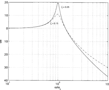
Figure 2-1 shows the helicopter in flight carrying the avionics box mounted on a custom suspension system to attenuate vibration inputs. High vibration levels significantly degrade performance of inertial sensors leading to high drift rates. Vibration also makes electronics more prone to failures, such as broken solder joints or loose connectors. There are several sources of vibration on a helicopter: the main rotor, the engine, the tail rotor, all of which can excite lightly damped structural modes, e.g. first bending mode of the tail boom. Data from an experiment with hard mounted inertial sensors have shown that the most important vibration source is the one-per-rev component from the main rotor, with the nominal frequency of 26.7 Hz. The suspension system consists of four neoprene isolators, located in the corners of a rectangle. The center of gravity of the suspended assembly is located at the center of the rectangle, which serves to decouple the translational modes and the rotational ones [10]. Neoprene has a low damping ratio ( = 0.05, which leads to fast decay of the transmissibility function, at the cost of a high peak at resonance (x10). The transmissibility function, depicted in Figure 2-2 for neoprene and another material with a higher damping ratio (( = 0.15), shows the ratio of the vibration amplitude of the suspended assembly to that of the base (airframe), given as a function of the ratio of the base vibration frequency to the natural frequency of the suspension system. According to Figure 2-2, for a low-damping material the airframe vibration inputs are attenuated

(18)

Figure 2-1: Instrumented X-Cell helicopter in flight

roughly by the square of the ratio, for a wide range of these ratios (e.g. 2-10). The choice of natural frequencies represents a tradeoff: the suspension should be flexible enough to provide adequate vibration isolation, but stiff enough to avoid coupling with the modes of interest for vehicle control. Note also that high transmissibility at resonance may lead to insufficient gain margin in a closed loop system. The gain margin problem can be alleviated by using digital notch filters at the resonant frequencies, but this leads to phase lag at lower frequencies, thereby reducing available bandwidth of the controllers. As a result, we chose desired frequencies to be in the range of 9 to 13 Hz. An additional requirement on the minimum stiffness is posed by aerobatics: the suspension system was designed to withstand 3 g's normal acceleration without bottoming out. The translational frequencies are set by the radial and axial spring stiffness ratings of the isolators given the mass of the assembly. The frequencies of the rotational modes are proportional to the distance between the isolators (and inversely proportional to the respective radii of inertia, determined with the effective torsional pendulum tests [10]). The isolators had to be located inside the box (see Figure 2-3) to achieve the desired frequencies.

For certain applications, like aerial imaging, superior vibration isolation can be achieved by using vibration mounts made of viscoelastic materials (Sorbothane, Barry-LT compound, etc), which feature higher damping ratios than neoprene. As can be seen in Figure 2-2, for a material with a damping ratio of 0.15, representative of a number of such materials, the transmissibility at resonance is reduced significantly (by a factor of 3), while it is increased only slightly at higher frequencies (e.g. at a frequency ratio of 3:1 the increase is by a factor of 1.28). Even in the absence of periodic inputs, the resonant frequency will be occasionally excited by step-like inputs from the pilot, or other disturbances (e.g. occasional engine sputtering), in which case the higher-damping materials will provide much better isolation.

(19)

101 10 0 101

Figure 2-2: Transmissibility function for different materials

2.2 Avionics system

Autonomous aerobatics calls for a high-bandwidth control system, which in turn necessi-tates fast servomechanisms, low latencies in the computers, and fast sensor response. The fastest actuator response is required for modulating the tail rotor pitch. We used a newly available digital servo, Futaba S9450, which features 7 Hz no-load small-signal bandwidth (i.e. frequency at which phase lag reaches 90 degrees). The torque on the tail rotor servo is small compared to the torque rating of the servo (105 oz.-in.), pitching inertia of the tail rotor blades is almost negligible, therefore the no-load bandwidth test is representative of its performance in flight. The main rotor actuators are older analog servos Futaba S9402. These servos were tested with a mean torque load of 35 oz.-in. (stall torque 111 oz.-in.) and a small inertial load. These tests resulted in an estimate of small-signal bandwidth of 5 Hz.

The core of the sensor suite was an inertial measurement unit (IMU) from Inertial Science [23]. It contains three gyroscopes and three accelerometers. The range of gyroscopes was set at

+300

deg/sec, and the range of accelerometers at ±5 g's. The helicopter with the payload is capable of achieving roll rates of 200 deg/sec, and yaw rates in excess of 1,000 deg/sec. The yaw rate command was limited in software to avoid sensor saturation and ensuing instability. The IMU had an internal power regulation, temperature compensation, serial output at 100 Hz and internal first order analog anti-aliasing filters, with the corner frequency set at 9 Hz. In hindsight, the frequency of the anti-aliasing filters should have been set higher, around 20 Hz, to reduce the phase lag at lower frequencies. The drift

(20)

5 7 8 910 13 13 12 List of Parts

1 Proxim Wireless LAN Adapter 2 Power Regulator

3 DSP Design TP300 PC 104 CPU 4 CMVC Superstar GPS Receiver 5 R/C Receiver & Battery its 6 Honeywell HPB200A Altimeter

7 Inertial Sciences ISIS IMU 8 MCU

2 9 Main Batteries

210 Servo Battery

11 Aluminum Enclosure

3 12 Mounting Bracket

13 ME500-1 Neoprene Isolators

(21)

rates of the gyroscopes were on the order of 0.02 deg/sec, and for accelerometers 0.02 g's for the duration of flight. To compensate for these low-frequency errors of the gyros and accelerometers, several more sensors were used to provide Kalman filter measurement updates.

A barometric altimeter, HPA200 from Honeywell, featured 2 ft resolution (0.001 psi), and excellent stability. Since the duration of flight was short, ambient pressure changes were negligible. The altimeter has an internal power regulation, temperature compensation and serial output, which was sampled at 5 Hz. Internally, pressure was sampled at 120 Hz, and averaged for 200 msec to produce the output. Since the altimeter is used to provide low-frequency updates, this effective delay was deemed tolerable. The altimeter and its pressure port were housed inside the avionics box, which shields the measurement from the pressure changes in the main rotor wake and from dynamic pressure induced by the vehicle motion and wind. It provides a reliable altitude measurement out of ground effect (about

2 rotor diameters, or 3 meters).

A Global Positioning System (GPS) receiver was used to provide 2-D (North and East) position and velocity updates. In the beginning a low-cost receiver with 1 Hz sampling period and 1 sec latency was used. A system of gravity-aiding complementary filters [47]

was used to estimate vehicle attitude, and velocity estimates were re-set each time a new GPS measurement was available. A triaxial magnetic compass was used to provide heading updates. An autonomous axial roll was performed with this suite, however the attitude and velocity estimates were rather crude. A high-end receiver, G12 from Ashtech, was installed. This receiver features 10 Hz update rate and maximum 50 msec latency. An Extended Kalman Filter (EKF), described in the next section, was implemented to provide a more accurate state estimate.

A low-cost triaxial magnetic compass, used for heading updates in the original sensor suite, was discarded. The magnetoresistive sensor required an external in-flight temperature and offset compensation provided by short duration high amplitude current pulses. The sensor provided analog outputs, and highly accurate voltage reference was used. Still, after the compensation and hard-iron calibration of the compass, the heading accuracy was around 15 degrees. The EKF with the updates from the low-latency receiver provided heading accuracy on the order of 6 degrees.

It is interesting to note that the development of a sensor suite in the university environ-ment is best impleenviron-mented with smart sensors, i.e. temperature compensated, with precise internal voltage reference, and providing a digital output. To develop a highly integrated, high performance sensor suite from low-cost components requires a significant investment into laboratory equipment, and development time. For a custom one-of-a-kind, or even a low-volume-production research unit it makes economic sense to pay extra for smart sensors. The best solution would be to use an off-the-shelf miniature avionics suite with adequate performance characteristics, however such a device has not been available on the market during the project.

Other avionic devices included a flight control computer (TP400 from DSP design, with a Pentium MMX 300 MHz compatible processor, ample random access and non-volatile memory and I/O), a wireless LAN transceiver, a remote-control (R/C) receiver for pilot commands, and a custom-designed servo board for sampling pilot commands and driving the servomechanisms at 50 Hz. The flight control processor ran the QNX 4.25 real-time operating system (RTOS) [25]. The software was implemented in the C programming language with multiple processes for modularity and, hence, ease of development and testing.

(22)

context switching time is the time it takes for the processor to switch from one process, or task, to another one). The most time-critical, and therefore the highest priority software process consisted of sampling the IMU (arrival of each serial port data packet triggered a hardware interrupt), running the estimation and control logic, and sending a serial message to the servo board to drive the actuators. Since the IMU sent data at 100 Hz, and the servos were driven at 50 Hz, this sequence was performed every second IMU message. A single execution of the estimation and control logic took less than 2 msec, thereby leaving roughly 18 msec out of each 20 msec interval for the lower-priority processes (measurement updates from GPS and altimeter, sampling battery voltage, telemetry, etc). In addition, it is beneficial to minimize the time lag from sampling the IMU to driving the servos to reduce phase lag. The IMU data transfer took 1.4 msec, servo command data transfer 2.6 msec, and all the servos were commanded in parallel for 2 milliseconds (the angle of a servo deflection is proportional to a commanded pulse width, which ranges from 1 to 2 msec). Therefore the pure time delay amounted to 8 msec, well below the servo control interval of 20 msec.

Radio frequency (RF) interference was addressed in the design. An aluminum box housing the avionics provided partial protection for the RF interference; and a semi-flexible antenna guide pointing downwards was used to put the antenna in the experimentally determined most favorable location. The guide was flexible enough to land on, and at the same time kept the antenna wire away from the main rotor blades during inverted flight.

By design the servo board, R/C receiver and the servos were electrically isolated from the rest of the avionics so that the pilot still could control the servos in case of the main computer failure. However, a small-scale helicopter like X-Cell is hard to fly at low speed without the yaw rate feedback to tail rotor pitch, because of the large tail rotor control sensitivity and small natural yaw damping. In moderately fast forward flight the helicopter becomes more manageable because of the weathercocking provided by the fin and the tail rotor, and the pilot could attempt a run-in landing.

The wireless datalink was used only to download telemetry information to the ground station, where the operator monitored the status of various indicators, such as the number of GPS satellites, battery voltage, attitude indicator, etc. No information was uploaded to the helicopter after the start of the program.

2.3 State estimation algorithm

Accurate state estimation was essential for modeling work, and the Extended Kalman Filter (EKF) is a commonly used means to achieve it by blending information from various sensors. The EKF used for helicopter state estimation employed a novel representation of attitude error, suggested by Frazzoli [12]. A robust and efficient numerical implementation of the filter is described below.

The nonlinear navigation equations contain sixteen states: north-east-down position (p),

north-east-down velocity (b), a 4-state quaternion representation of attitude (q), and 3D vectors of acceleration biases (4b) and gyro biases (C4). The quaternion is free of singularities associated with the attitude representation based on the three Euler angles, but is subject to a unit norm constraint [46]. Denote accelerometer readings by am and gyro readings W.

Then the navigation equations are:

(23)

v = C(am-&b)+ 0 9 (2.2) 1

q = - 2 m

A

4+ k4 (2.3)

b = 0 (2.4)

Wb = 0 (2.5)

where C is the direction cosine matrix transforming body axis coordinates to the North-East-Down (NED) system, Qm and !b are 4 x 4 skew-symmetric matrices [48] composed of the gyro measurements and gyro bias estimates, A = 1 - ||qll2 is a deviation of the square of the quaternion norm from unity due to numerical integration errors, and k is the factor that determines the convergence speed of the numerical error. These factors serve the role of Lagrange multipliers ensuring that the norm of the quaternion remains close to unity [46]. The constraint on the speed of convergence for stability of the numerical solution is k - dt < 1, where dt is the integration time step. The quaternion propagation equation can be discretized with an analytical computation of the exponent of the skew-symmetric matrix, given by Stevens [48]. The discrete-time attitude update can be written as:

q(t + dt) = exp - Q - dt q(t) (2.6)

Denote

#

w - dt -an effective rotation, undergone by the body during the time period of dt, assuming that the angular rate w remained constant during the interval. Accordingly, introduce the 4 x 4 skew-symmetric matrix 4 = Q -dt:

0 #2 #y #2

4 =(# _-4y 0 -#z #y 2.7)

Oz 0 -4X

-#z -d #5 O 0

Then, using the idempotent property of the 4 x 4 skew symmetric matrices, we get:

11 sins (28

exp (-4)4 = I cos s - -44 (2.8)

2 2 s

where s =

l|#||.

Eqs. (2.6) and (2.8) ensure in theory that the updated quaternion q(t

+

dt) has a unit norm. However, a small Lagrange multiplier term was added to Eq. (2.8) to maintain numerical stability. The use of the Lagrange multiplier term relaxes the requirement on the accuracy of computation of the trigonometric functions, and allows us to use truncated series for cos(s) and sin(s)/s.

q(t + dt) I (cos s + k - dt - A) - 14 S _S2 _{8 1}q(t) (2.9) Eq. (2.9) and discrete-time counterparts of the velocity and position propagation equations ((2.1) and (2.2)) were integrated each time a new IMU measurement arrived, i.e. every 10 msec.

The differential equations for the state estimation error are obtained by linearizing Eqs. (2.1)-(2.5) around the current state estimate [45]. The resulting Jacobian matrix is used to

(24)

propagate the covariance matrix. The upper-triangular square root time update algorithm based on Householder orthogonalization procedure was used for higher precision [34]. The algorithm was optimized to gain speed from the sparseness of the Jacobian matrix, and the time to run the time update (by far the most expensive computation in the entire flight software) took less than 2 msec during each 20 msec control cycle.

The linear error model contains 15 states: 3D position (p), 3D velocity (v), 3D attitude error representation (#), and 3D vectors for bias estimation errors for accelerometers (n)

and gyros (p). Note that whereas the attitude vector is represented by a 4-dimensional quaternion with the unit norm constraint, the attitude error vector is three dimensional. This allows us to perform an unconstrained estimation of the attitude error. A number of 3D attitude error representations have been suggested, and a survey can be found in ref. [29]. A commonly used attitude error representation [45] is given first in the following. Let C be the true direction cosine matrix, and 4 be a 3 x 3 skew-symmetric matrix, whose components

#, #y,

and

#z

represent small rotations around each of the body axis. Note also that D, given in Eq. (2.10), represents a vector product matrix, such that for a vector a

C

R3 we have 4Da = (Ox)a = -(ax)o.

0 -#z

4Y

0 -#X (2.10)

-#Y #2 0

Then the relation between the true and estimated direction cosine matrices is represented as

C ~ C (I+ D) (2.11)

The measurement update step provides an estimate of the attitude error vector

#.

Eq. (2.11) is then used to generate a new estimate of the direction cosine matrix, and, hence, the quaternion. However, the orthogonality property of the direction cosine matrix is lost in the update given by Eq. (2.11). An explicit orthogonalization step is required [45], introducing another source of error, and increasing computational burden. The errors introduced by the orthogonalization step grow with the magnitude of the correction, and will be most noticeable in tasks such as an in-flight alignment (attitude determination after a crude initialization). Another common 3D attitude error representation is the Gibbs vector [20], based directly on the variation of the attitude quaternion, rather than the direction cosine matrix. It also requires a normalization step after the measurement update to preserve the unit norm of the quaternion [33].

Following Frazzoli [12], instead of Eq. (2.11), the attitude error can be represented by Eq. (2.12).

C = C exp (1) (2.12)

This is equivalent to

q = exp 4 q (2.13)

given that the same 3D attitude error vector (#) is used for the elements of matrix I4 (Eq. (2.7)). To see the equivalence, consider attitude propagation equations based on the direction cosine and quaternion representations.

(25)

1 44 _(2.15) 2

Assume that the angular rate vector w is constant during a time interval t, and denote

#=

wt. Then, provided the initial attitude represented by Co or qo, the solutions of the differential equations (2.14) - (2.15) are:

C(t) = Co exp (D) q(t) = exp (- 4 qo

Clearly, C(t) and q(t) represent the same attitude.

The attitude error representation in Eq. (2.12) maintains the orthogonality of the direction cosine matrix:

CCT =

0

exp (4) (exp (+))TOT =Oexp(+)exp(-4)OT =Oexp( - 5)OT = I (2.16)

At the same time the linearization of Eq. (2.12) leads to Eq. (2.11), therefore the linear equations for time propagation of the state estimation error do not change. They are given in Eqs. (2.17)-(2.19).

p= v (2.17)

=

O(&x)#-Oi+O

_(2.18)

= -(Ox)#+pA+-Y (2.19)

Here & = (am - 1b) and Z = (Pm - b) are accelerometer and gyro measurements with the current bias estimates subtracted, 7 and -y are random noise components of accelerometer and gyro measurement errors, n and p are bias estimate errors, modeled as random walks [19] according to the linearization of Eqs. (2.4) and (2.5).

Let us provide the derivations for velocity and attitude error propagation equations, given in Eqs. (2.18) and (2.19), respectively. Denote by V the true inertial velocity vector, the differential equation for which is:

Y

= C (a, - ab - 7) (2.20)

Subtract Eq. (2.20) from Eq. (2.2), and neglecting second order terms with respect to the error vector we obtain:

v = - V=C(am-b)-C(am-ab--7)

=

0(am-&b)-C(a,-&b)+C(am-&b)-C(am-ab-,)

= 0 -O-C)±(am-CC+ C77

=

O(ax)#-OK+

Oq

Attitude propagation can be alternatively expressed with the derivative of the direction cosine matrix, resulting in the counterpart of Eq. (2.3):

(26)

Similarly, we can express the derivative of the true direction cosine matrix:

6

= C (Qr - Qb+ F) (2.22)

where F is a skew symmetric matrix composed of the elements of the gyro noise vector (y). Next, subtract Eq. (2.22) from Eq. (2.21), and neglect second-order terms:

O-c

0

(m -b - C (m - Qb+ rF)-= (m -C (Qm -)+C ( -)-- C (m Qb -C F ->

O

(Qm - 2b)D -

O6=-$

(m - (b) -CM - C F 4)(Qm -b) Qn- 0b>I)+ M±+ r # = -

(6^x)#+

P +-Y

Here M is a skew symmetric matrix composed of the elements of the gyro bias estimation error (p).

The measurement update step remains the same until the incorporation of the computed attitude correction. Pressure altitude, 2D GPS position and 2D GPS velocity measurements were used. The updates were implemented with a fast upper triangular square root algo-rithm developed by Carlson [5, 34]. The method improves numerical stability of the classical measurement update step by substituting the inversion of a potentially ill-conditioned sym-metric matrix with the inversion of its square root. The method maintains the square root of the covariance matrix in the upper triangular form, and was shown to incur small computational penalty compared with the original algorithm [5].

After the state error vector is calculated, the navigation filter states from the Eqs. (2.1)-(2.5) are updated. To incorporate the attitude correction (#) into the quaternion estimate, we use Eq. (2.13), calculating the skew-symmetric matrix exponent analytically according to Eq. (2.8). This algorithm ensures that the quaternion norm remains equal to unity without an additional normalization step. It is also computationally more efficient than first calculating an updated direction cosine matrix from Eq. (2.12) and then finding the quaternion vector that corresponds to it.

The source of attitude updates comes from the 2D GPS position and velocity mea-surements. Note that the heading error becomes unobservable when the resultant of the non-gravity forces acting on the body (measured by accelerometers) is aligned with the local vertical [51]. To show this, let us rearrange the velocity error propagation equation in Eq. (2.18):

=Ox r

O#-O

O+x4-

O

+07

(2.23)

where &n represents a vector of forces acting on the body in the NED coordinate frame, and

#1

=

#

6=

)4@ is the attitude error vector expressed in the NED frame. From

the vector product in Eq. (2.23) it follows that if &I is aligned with the local vertical, 64' becomes unobservable. Therefore, some maneuvering is required for convergence of the heading error. This constraint did not represent a problem for the particular task at hand (autonomous aggressive maneuvering), however for applications requiring a prolonged

(27)

continuous hover or flight along a straight line an additional source of heading measurement would be needed.

Such a source is usually provided by a magnetometer, which measures a projection of the Earth magnetic field vector on the body axes. The measurement equation for a magnetometer with three sensitive axes is:

Z=ob+v , (2.24)

where b represents a known local magnetic field vector, and v is the measurement noise. Therefore the error equation for the measurement is

z = (0 - C) b+v = -O ($x) b+v (2.25)

From Eq. (2.25) we can see that the rotation angle around the magnetic field vector does not contribute to the measurement. In the absence of the gyro and numerical errors an initial error rotation angle around the magnetic vector will remain constant. To show this, consider propagation of the attitude error under these conditions. Denote an initial attitude error vector by 0. Then

C(to) =

O(to)

exp((o)

Since ideal gyro measurements are assumed, the estimate of the direction cosine matrix is propagated according to the same differential equation as the true one, with different initial conditions:

C

=

CQ

Integrating the attitude matrix propagation equations 0(t) =

0(to)F(t,to)

C(t) = C(to)F(t, to) = 0(to) exp(4o)F(t, to) where F(t,to) = exp (jt (r)dT)

At the same time:

C(t) = 0(t) exp(1(t)) Hence, observing that F(t, to) is an orthogonal matrix:

exp(D(t)) = FT (t, to) exp(1o)F(t, to) (2.26) Eq. (2.26) shows that the attitude error follows coordinate transformation rules, therefore

0

and

#(t)

represent the same attitude error vector, expressed in the original and current coordinate systems. Therefore, if

#o

represents a rotation around the magnetic field vector, this error will not be changed by the magnetometer measurement updates.

Thus a magnetometer, like a star-tracker in a satellite, provides effectively two attitude angles (albeit not aligned with any of the Euler angles). Obviously, the utility of the magnetometer measurement udpate for estimating attitude depends highly on the accuracy of the local magnetic field measurement. Prominent factors affecting the accuracy are

(28)

VISUALIZATION COMPUTER SERVO RACK SIMULATION COMPUTER

ETHERNET AID CONVERTER

RPM SERIAL PORTS DIA CONVERTER

RUDDER IMUll 1111GPS COMPASS E LEVATO ALTIMETER AILERON COLLECTIVE SERVO COMMANDS DIRECT CONNECTION PILOT INPUTS

SERVO BOARD ONBOARD CLONE GROUND STATION

PILOT INPUTS

R/C RECEIVER R/C TRANSMITTER

Figure 2-4: Hardware-in-the-loop simulation

temperature drifts and the magnetic field imposed by the helicopter and its payload. A combination of hardware solutions and hard-iron calibration, applied to a high-end magnetic sensor can result in accurate two-component attitude updates.

2.4 Hardware-in-the-loop simulation

An essential tool in the development of a real-time control system is a hardware-in-the-loop simulation (HILSim). It allows the engineer to test the actual software running on the target hardware in conditions as close to a real flight as is achievable in the lab.

Figure 2-4 presents a diagram of the HILSim. The so-called "clone" computer is a copy of the flight control computer running the same software; the servo board, R/C receiver and servomechanisms are also exact copies of their counterparts on the helicopter. The commands coming from the pilot get delivered to the clone via the servo board. The control logic in the clone generates servo commands based on the pilot commands and modeled sensor inputs from the simulation computer, and delivers them back to the servo board. The servo board drives the servos, their positions are sampled at 100 Hz by the simulation computer via potentiometers. In the servo rack the second row of servos represents the potentiometers (low-cost servos with the electric motors removed). The simulation computer interprets servo deflections as corresponding actuator commands, and integrates equations

(29)

of motion accordingly. It then generates sensor models based on the computed state vector and a priori models of sensor errors, and feeds these data to the clone via the interfaces the latter expects. The HILSim captures the latencies inherent in the system, an essential feature for testing real-time software.

Ideally, the servomechanisms should be appropriately spring- and inertia- loaded to simulate the effect of these factors on bandwidth. As was mentioned earlier, the actuator with the most stringent requirement for bandwidth is the tail rotor pitch, which is very lightly loaded. Therefore, we did not use loading to extend the lifetime of the servos. This deficiency of the HILSim was taken into account when the control system was designed: additional phase margin was built in.

(30)

(31)

Chapter 3 Dynamic model of a miniature

helicopter

3.1 Overview of Modeling Approaches

There exists an extensive body of literature on the dynamics of full-scale helicopters. Step-by-step procedures for developing first-principles dynamic models have been devised and published [44, 2, 49, 22]. The models used in full-scale helicopter simulators typically are high-order and contain a large number of parameters that often cannot be measured directly. Moreover, once developed, models require extensive validation and refinement until they can predict the vehicle dynamic behavior accurately. Applying detailed modeling techniques is therefore not a trivial task, and may not be warranted given the differences between full-scale and miniature helicopters. Helicopters evolve in a wide range of aerodynamic conditions. Complex interactions take place between the rotor wake and the fuselage or tail. In miniature helicopters, these subtle effects tend to be "overpowered" by the large rotor forces and moments that follow quasi-instantaneously the rotor control inputs. To the author's knowledge, no examples of helicopter models covering aerobatic conditions have been published prior to this work.

Modeling techniques based on system identification have been used to derive linear models for control design, study the vehicle flying qualities, and for the validation and refinement of detailed non-linear first-principle models. Frequency domain identification methods such as CIFER [43, 50], were used to derive relatively simple linear parameterized models that capture high-frequency range of the vehicle dynamics around specific operating points. These models poorly describe lower-frequency modes because of necessary pilot's feedback during data gathering flights. Linear models are also inadequate for simulating many aspects of aerobatic flight because of the large deviations of state variables (attitudes, angular rates, and velocities) from the trim conditions.

Mettler [37] applied frequency-domain systems identification methods (CIFER) to study the characteristics of small-scale helicopters. He developed and identified parameterized lin-ear models for hover and cruise flight conditions for the Yamaha R-50 (a 10 ft rotor diameter, 150 lb helicopter). He later applied the same parameterized model to MIT's X-Cell .60, val-idating and extending the observation that the rotor forces and moments largely dominate the dynamic response of small-scale helicopters. This significantly simplifies the modeling task. Both flight conditions are accurately modeled by a rigid-body model augmented with the first-order rotor and stabilizer bar dynamics; no inflow dynamics were necessary. The

(32)

coupled rotor and stabilizer bar equations can be lumped into one first-order effective rotor equation of motion (for both the lateral and longitudinal tip-path-plane flapping). The lin-ear models accurately capture the vehicle dynamics for a relatively large region around the nominal operating point. The model accurately predicts the vehicle angular rate response for aggressive control inputs.

Following the work by Mettler, LaCivita et al. [28] developed a technique that makes use of the frequency responses identified from multiple operating points, for the identification of key parameters of a more broadly descriptive non-linear model. He applied the technique to Yamaha R-50 helicopter using the hover and cruise data collected in [37]. The nonlinear model with 30 states is linearized to permit a fit with the local frequency responses. It was also shown that the reduced-order linearized model, similar to the one proposed by Mettler [37], provides practically the same level of accuracy, further validating proposed simple structure of a dynamic model for miniature helicopters.

The model has typical rigid body states with the quaternion attitude representation used in order to enable simulation of extreme attitudes [46], two states for the lateral and longitudinal flapping angles, one for the rotorspeed, and one for the integral of the ro-torspeed tracking error. This last state comes from the governor action, modeled with a proportional-integral feedback from the rotorspeed tracking error to the throttle command. The model covers a large portion of the X-Cell's natural flight envelope: from hover flight to about 20 m/sec forward flight. The maximum forward speed corresponds to an advance ratio y = 0.15, which is considered as relatively low [44], and permits a number of as-sumptions (e.g. thrust perpendicular to the rotor disk, see [6]). The cross-coupling effects in the rotor hub were also shown to be negligible for this helicopter, which further sim-plified model development. The mathematical model was developed using basic helicopter theory, accounting for the particular characteristics of a miniature helicopter. Most of the parameters were measured directly, several were estimated using data collected from simple flight-test experiments, involving step and pulse responses in various actuator inputs. No formal system identification procedures are required for the proposed model structure. The model's accuracy was verified using comparison between model predicted responses and responses collected during flight test data. The model was also "flown" by an expert RC pilot to determine how well it reproduces the piloted flying qualities.

Analytical linearization of the model with respect to forward speed was used to derive simple linear models. These were subsequently used for a model-based design of the con-trollers used for the automatic execution of aerobatic maneuvers. The actual aggressive trajectories flown by the helicopter were adequately predicted by the simulation based on the developed nonlinear model.

In the remainder of the chapter we provide a full list of model parameters with the numerical values, dynamics equations of motion, and expressions for forces and moments exerted on the helicopter by its components. Throughout the chapter we provided flight test data to validate the model for various flight regimes, including aerobatics.

3.2 Helicopter parameters

The physical helicopter parameters used for our model are given in Table 3.1. The moments of inertia around the aircraft body axes passing through the vehicle center of gravity were determined using torsional pendulum tests [10]. The cross-axis moments of inertia are hard to measure without a balancing device; and since they are usually small they were

(33)

neglected. The X-Cell main and tail rotors, as well as the stabilizer bar, have symmetric airfoils. The lift curve slopes of these surfaces were estimated according to their respective aspect ratios [26]. The effective torsional stiffness in the hub was estimated from angular rate responses to step commands in cyclic, as described in Section 3.4.1.

Note that in the table "m.r." stands for the main rotor, "t.r." stands for the tail rotor.

3.3 Equations of motion

The rigid body equations of motion for a helicopter are given by the Newton-Euler equations shown below. Here the cross products of inertia are neglected.

6 = vr -wq-gsin0+(Xmr+XfuS)/m

v = wp-ur+gsin bcos0+(Ymr+Yfus+Ytr+Yvf)/m

b = uq-vp+gcosbcos0+(Zmr+Zfus+Zht)/m = qr(Iyy - Izz)/Ixx + (Lmr + Lvf + Ltr) /Itx = pr(Izz - Ixx)/Iyy + (Mmr + Mht) /'yy

= pq(Ixx - Iyy)/Izz + (-Qe + Nv5 + Ntr) /Izz

The set of forces and moments acting on the helicopter are organized by components: ()mr for the main rotor; Otr for the tail rotor; ()fus for the fuselage (includes fuselage aerodynamic effects); (),f for the vertical fin and ()ht for the horizontal stabilizer. These forces and moments are shown along with the main helicopter variables in Fig. 3-1. Qe is

the torque produced by the engine to counteract the aerodynamic torque on the main rotor blades. The helicopter blades rotate clockwise when viewed from above, therefore Qe > 0. In the above equations we assumed that the fuselage center of pressure coincides with the c.g., therefore the moments created by the fuselage aerodynamic forces were neglected. The rotational kinematic equations were mechanized using quaternions [46]. The inertial velocities are derived from the body-axis velocities by a coordinate transformation (fiat Earth equations are used), and integrated to obtain inertial position. A 4th order

Runge-Kutta integration method is used, with an integration step of 0.01 seconds.

3.4 Component forces and moments

3.4.1 Main rotor forces and moments Thrust

For the main rotor thrust we assumed that the inflow is steady and uniform. According to Padfield [44, p. 126], the time constant for settling of the inflow transients at hover is given by

0.849

TA = 4 4 9 (3.1)

Atrim mr

For our helicopter the induced velocity at hover trim condition can be determined from simple momentum theory:

Vimr g - 4.2 m/sec (3.2)

Autonomous aerobatic maneuvering of miniature helicopters