Below P vs NP: Fine-Grained Hardness for
Big Data Problems
by
Arturs Backurs
B.S., University of Latvia (2012)
S.M., Massachusetts Institute of Technology (2014)
Submitted to the Department of Electrical Engineering and Computer
Science
in partial fulfillment of the requirements for the degree of
Doctor of Philosophy
at the
MASSACHUSETTS INSTITUTE OF TECHNOLOGY
September 2018
c
○ Massachusetts Institute of Technology 2018. All rights reserved.
Author . . . .
Department of Electrical Engineering and Computer Science
August 30, 2018
Certified by . . . .
Piotr Indyk
Professor of Electrical Engineering and Computer Science
Thesis Supervisor
Accepted by . . . .
Leslie A. Kolodziejski
Professor of Electrical Engineering and Computer Science
Chair, Department Committee on Graduate Students
Below P vs NP: Fine-Grained Hardness for
Big Data Problems
by
Arturs Backurs
Submitted to the Department of Electrical Engineering and Computer Science on August 30, 2018, in partial fulfillment of the
requirements for the degree of Doctor of Philosophy
Abstract
The theory of NP-hardness has been remarkably successful in identifying problems that are unlikely to be solvable in polynomial time. However, many other important problems do have polynomial-time algorithms, but large exponents in their runtime bounds can make them inefficient in practice. For example, quadratic-time algorithms, although practical on moderately sized inputs, can become inefficient on big data problems that involve gigabytes or more of data. Although for many data analysis problems no sub-quadratic time algorithms are known, any evidence of quadratic-time hardness has remained elusive.
In this thesis we present hardness results for several text analysis and machine learning tasks:
∙ Lower bounds for edit distance, regular expression matching and other pattern matching and string processing problems.
∙ Lower bounds for empirical risk minimization such as kernel support vectors machines and other kernel machine learning problems.
All of these problems have polynomial time algorithms, but despite extensive amount of research, no near-linear time algorithms have been found. We show that, under a natural complexity-theoretic conjecture, such algorithms do not exist. We also show how these lower bounds have inspired the development of efficient algorithms for some variants of these problems.
Thesis Supervisor: Piotr Indyk
Acknowledgments
First and foremost, I would like to thank my advisor Piotr Indyk for the guidance and support that he provided during my graduate studies.
I thank Costis Daskalakis and Virginia Vassilevska Williams for serving on my thesis committee.
I would also like to say thank you to all people from Piotr’s group, in particular, Sepideh Mahabadi, Ilya Razenshteyn, Ludwig Schmidt, Ali Vakilian and Tal Wagner for all that I learned from them.
I am grateful to Andris Ambainis who introduced me to theoretical computer science. I thank Krzysztof Onak and Baruch Schieber for hosting me at IBM during my summer internship in 2015.
Finally, I thank my past and current collaborators: Amir Abboud, Kyriakos Axiotis, Mohammad Bavarian, Karl Bringmann, Moses Charikar, Nishanth Dikkala, Thomas Dueholm Hansen, Piotr Indyk, Marvin Künnemann, Cameron Musco, Krzysztof Onak, Mădălina Persu, Eric Price, Liam Roditty, Baruch Schieber, Ludwig Schmidt, Gilad Segal, Anastasios Sidiropoulos, Paris Siminelakis, Christos Tzamos, Ali Vakilian, Tal Wagner, Nicole Wein, Ryan Williams, Virginia Vassilevska Williams, David P. Woodruff, Or Zamir.
Contents
Acknowledgments 5 Contents 7 List of Figures 11 List of Tables 13 1 Introduction 151.1 Main contributions: an overview . . . 16
1.2 Hardness assumption . . . 17
1.3 Pattern matching and text analysis . . . 18
1.3.1 Hardness for sequence alignment problems . . . 18
1.3.2 Regular expression pattern matching and membership . . . 20
1.4 Statistical data analysis and machine learning . . . 21
1.4.1 Kernel methods and neural networks . . . 21
1.4.2 Efficient density evaluation for smooth kernels . . . 22
2 Preliminaries 23
I
Pattern matching and text analysis
27
3 Edit distance 29 3.1 Preliminaries . . . 293.2 Reductions . . . 30
3.2.1 Vector gadgets . . . 30
3.2.2 Properties of the vector gadgets . . . 32
3.2.3 Hardness for pattern matching . . . 35
3.2.4 Hardness for edit distance . . . 37
3.2.5 Reduction from the almost orthogonal vectors problem . . . . 38
4 Longest common subsequence and dynamic time warping 39 4.1 Preliminaries . . . 40
4.2 Hardness for longest common subsequence . . . 41
4.2.2 Reducing the almost orthogonal vectors problem to LCS . . . 43
4.3 Hardness for dynamic time warping . . . 48
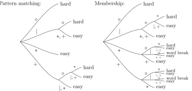
5 Regular expressions 51 5.1 Preliminaries . . . 58
5.2 Reductions for the pattern matching problem . . . 59
5.2.1 Hardness for type “|∘|” . . . 60
5.2.2 Hardness for type “|∘+” . . . 61
5.2.3 Hardness for type “∘*” . . . 62
5.2.4 Hardness for type “∘+∘” . . . 65
5.2.5 Hardness for type “∘|∘” . . . 68
5.2.6 Hardness for type “∘+|” . . . 69
5.2.7 Hardness for type “∘|+” . . . 71
5.3 Reductions for the membership problem . . . 72
5.3.1 Hardness for type “∘*” . . . 72
5.3.2 Hardness for type “∘+∘” . . . 72
5.3.3 Hardness for type “∘|∘” . . . 74
5.3.4 Hardness for type “∘+|” . . . 74
5.3.5 Hardness for type “∘|+” . . . 75
5.4 Algorithms . . . 76
5.4.1 Algorithm for the word break problem . . . 76
5.4.2 Algorithm for type “∘+” . . . 81
5.4.3 Algorithms for types “|*∘” and “|+∘” . . . 82
5.4.4 Algorithms for types “|∘+” and “*∘+” . . . 83
6 Hardness of approximation 85 6.1 Our results . . . 85
6.2 Valiant series-parallel circuits . . . 87
6.3 VSP circuits and the orthogonal row problem . . . 90
6.4 The reduction to approximate LCS . . . 93
6.5 Hardness for binary LCS and edit distance . . . 100
II
Statistical data analysis and machine learning
102
7 Empirical risk minimization 103 7.1 Our contributions . . . 1047.1.1 Kernel ERM problems . . . 104
7.1.2 Neural network ERM problems . . . 105
7.1.3 Gradient computation . . . 106
7.1.4 Related work . . . 106
7.2 Preliminaries . . . 107
7.3 Hardness for kernel SVM . . . 108
7.3.1 Hardness for SVM without the bias term . . . 108
7.3.3 Hardness for soft-margin SVM . . . 118
7.4 Hardness for kernel ridge regression . . . 119
7.5 Hardness for kernel PCA . . . 121
7.6 Hardness for training the final layer . . . 122
7.7 Gradient computation . . . 125
7.8 Conclusions . . . 128
8 Kernel density evaluation 131 8.1 Our results . . . 132
8.2 Preliminaries . . . 133
8.3 Algorithm for kernel density evaluation . . . 134
8.4 Removing the aspect ratio . . . 138
8.5 Algorithms via embeddings . . . 140
8.5.1 A useful tool . . . 140
8.5.2 Algorithms . . . 140
8.6 Hardness for kernel density evaluation . . . 142
List of Figures
3-1 Visualization of the vector gadgets . . . 31 5-1 Tree diagrams for depth-3 expressions . . . 56 5-2 Visualization of the preprocessing phase . . . 80
List of Tables
5.1 Classification of the complexity of depth-2 expressions . . . 54 5.2 Classification of the complexity of depth-3 expressions . . . 55
Chapter 1
Introduction
Classically, an algorithm is called “efficient” if its runtime is bounded by a polynomial function of its input size. Many well-known computational problems are amenable to such algorithms. For others, such as satisfiability of logical formulas (SAT), no polynomial time algorithms are not known. Although we do not know how to prove that no such algorithm exists, its non-existence can be explained by the fact that SAT is NP-hard. That is, a polynomial-time algorithm for SAT would imply that the widely believed P ̸= NP hypothesis is false. Thus, no polynomial-time algorithm for SAT and other NP-hard problems exists, as long as P ̸= NP.
As the data becomes large, however, even polynomial time algorithms often cannot be considered “efficient”. For example, a quadratic-time algorithm can easily take hundreds of CPU-years on inputs of gigabyte size. For even larger (say terabyte-size) inputs, the running time of an “efficient” algorithm must be effectively linear. For many problems such algorithms exist; for others, despite decades of effort, no such algorithms has been discovered so far. Unlike for SAT, however, an explanation for the lack of efficient solutions is hard to come by, even assuming P ̸= NP. This is because the class 𝑃 puts all problems solvable in polynomial time into one equivalence class, not making any distinctions between different exponents in their runtime bounds. Thus, in order to distinguish between, say, linear, quadratic or cubic running times, one needs stronger hardness assumptions, as well as efficient reduction techniques that transfer hardness from the assumptions to the problems. Over the last few years, these research directions has been a focus of an emerging field of fine-grained complexity.
The goal of this thesis is to investigate the fine-grained complexity of several funda-mental computational problems, by developing conditional lower bounds under strong yet plausible complexity-theoretic assumptions. On a high level, the implications of our results are two-fold. On the one hand, a lower bound that matches a known upper bound gives an evidence that a faster algorithm is not possible or at least demonstrates a barrier for a further improvement. On the other hand, the lack of conditional hardness for a problem suggests that a better algorithm might be possible. Indeed, in this thesis we present several new algorithms inspired by this approach.
1.1
Main contributions: an overview
Here we will give an overview of the main contributions. We describe the results in more detail in the subsequent sections.
Sequence similarity and pattern matching Measuring (dis)-similarity between sequences and searching for patterns in a large data corpus are basic building blocks for many data analysis problems, including computational biology and natural language processing. In this thesis we study the fine-grained complexity of these problems. First, we show a conditional (nearly) quadratic-time lower bound for computing the edit distance between two sequences. The edit distance (a.k.a. the Levenshtein distance) between two sequences is equal to the minimum number of symbol insertions, deletions and substitutions needed to transform the first sequence into the second. This is a classical computational task with a well-known quadratic-time algorithm based on dynamic programming. Our hardness result is the first complexity-theoretic evidence that this runtime is essentially optimal.
The techniques developed for this problem allows us to show computational hard-ness for several other similarity measures, such as the longest common subsequence and dynamic time warping. We also give evidence that some of those computational tasks are hard to solve even approximately, at least for deterministic algorithms. Finally, we also study pattern matching with regular expressions. In turn, this study has led to faster algorithms for the word break problem, a popular interview question.
This part of the thesis is based on the following papers:
∙ Arturs Backurs, Piotr Indyk, Edit Distance Cannot Be Computed in Strongly Subquadratic Time (unless SETH is false), appeared at STOC 2015 and HALG 2016 [BI15]. Accepted to the special issue of the SIAM Journal of Computing. ∙ Arturs Backurs, Amir Abboud, Virginia Vassilevska Williams, Tight Hardness
Results for LCS and Other Sequence Similarity Measures, appeared at FOCS 2015 [ABVW15].
∙ Arturs Backurs, Amir Abboud, Towards Hardness of Approximation for Poly-nomial Time Problems, appeared at ITCS 2017 [AB17].
∙ Arturs Backurs, Piotr Indyk, Which Regular Expression Patterns are Hard to Match?, appeared at FOCS 2016 [BI16].
Statistical data analysis and machine learning In the second part of this thesis we study the complexity of a number of commonly used machine learning problems and subroutines, all of which are solvable in polynomial time. These include a collection of kernel problems, such as support vector machines (SVMs) and density estimation, as well as (batch) gradient evaluation in neural networks. We show that, in the typical case when the underlying kernel is Gaussian or exponentially decaying, all of those problems require essentially quadratic time to solve up to high accuracy. In contrast,
we give a nearly-linear-time algorithm for density estimation for kernel functions with polynomial decay.
This part of the thesis is based on the following two papers:
∙ Arturs Backurs, Piotr Indyk, Ludwig Schmidt, On the Fine-Grained Complexity of Empirical Risk Minimization: Kernel Methods and Neural Networks, appeared
at NIPS 2017 [BIS17].
∙ Arturs Backurs, Moses Charikar, Piotr Indyk, Paris Siminelakis, Efficient Den-sity Evaluation for Smooth Kernels, to appear at FOCS 2018 [BCIS18].
1.2
Hardness assumption
Given a problem that is solvable in quadratic 𝑂(𝑛2) time, how can we argue that it
cannot be solved in a strongly sub-quadratic 𝑂(𝑛2−𝜀) time, for a constant 𝜀 > 0? As we discussed above, the P ̸= NP conjecture seems to be insufficient for this purpose, as it does not make a distinction between problems that are solvable in linear time and those that require quadratic time. Thus, we need a stronger hardness assumption to achieve such separations.
One such commonly used hardness assumption is known as the Strong Exponential Time Hypothesis (SETH) [IPZ01, IP01]. SETH is a statement about the complexity of the 𝑘-SAT problem: decide whether a given conjunctive normal form formula on 𝑁 variables and 𝑀 clauses, where each clause has at most 𝑘 literals, is satisfiable. It postulates that 𝑘-SAT cannot be solved in time 𝑂(︀2(1−𝜀)𝑁)︀ where 𝜀 > 0 is a constant
independent of 𝑘. In contrast, despite decades of research, the best known algorithm for 𝑘-SAT runs in time 2𝑁 −𝑁/𝑂(𝑘) (e.g., [PPSZ05]), so the constant in the exponent approaches 1 for large 𝑘. Thus, SETH is a strengthening of the P ̸= NP hypothesis, as the latter merely states that the satisfiability problem cannot be solved in polynomial time. Over the last few years, the hypothesis has served as the basis for proving conditional lower bounds for several important computational problems, including the diameter in sparse graphs [RVW13, CLR+14], local alignment [AVWW14], dynamic
graph problems [AVW14], Fréchet distance [Bri14], and the approximate nearest neighbor search [Rub18].
Many of the aforementioned are in fact obtained via a reduction from an interme-diary problem, known as the Orthogonal Vectors Problem (OVP), whose hardness is implied by SETH. It is defined as follows. Given two sets 𝐴, 𝐵 ⊆ {0, 1}𝑑 such that
|𝐴| = |𝐵| = 𝑁 , the goal is to determine whether there exists a pair of vectors 𝑎 ∈ 𝐴 and 𝑏 ∈ 𝐵 such that the dot product 𝑎 · 𝑏 = ∑︀𝑑
𝑖=1𝑎𝑖𝑏𝑖 (taken over reals) is equal to
0, that is, the vectors are orthogonal. An alternative formulation of this problem is: given two collections of 𝑁 sets each, determine if there is a set in the first collection that does not intersect a set from the second collection.1 A strongly subquadratic-time
algorithm for OVP, i.e., with a running time of 𝑂(𝑑𝑂(1)𝑁2−𝛿), would imply that SETH
1Equivalently, after complementing sets from the second collection, determine if there is a set in
is false, even in the setting 𝑑 = 𝜔(log 𝑁 ). In this thesis we adopt this approach and obtain our conditional hardness results via reductions from OVP.
1.3
Pattern matching and text analysis
1.3.1
Hardness for sequence alignment problems
The edit distance measures the similarity of two input sequences and is defined as the minimum number of insertions, deletions or substitutions of symbols needed to transform one sequence into another. The metric and its generalizations are widely used in computational biology, text processing, information theory and other fields. In particular, in computational biology it can be used to identify regions of similarity between DNA sequences that may be due to functional, structural, or evolutionary relationships [Gus97]. The problem of computing the edit distance between two sequences is a classical computational task, with a well-known algorithm based on the dynamic programming. Unfortunately, that algorithm runs in quadratic time, which is prohibitive for long sequences.2 A considerable effort has been invested into designing faster algorithms, either by assuming that the edit distance is bounded, by considering the average case or by resorting to approximation.3 However, the
fastest known exact algorithm, due to [MP80, BFC08, Gra16], has a running time of 𝑂(𝑛2(log log 𝑛)/ log2𝑛) for sequences of length 𝑛, which is still nearly quadratic.
In this thesis we provide evidence that the (near)-quadratic running time bounds known for this problem might, in fact, be tight. Specifically, we show that if the edit distance can be computed in time 𝑂(𝑛2−𝜀) for some constant 𝜀 > 0, then the Orthogonal Vectors Problem can be solved in 𝑂(𝑑𝑂(1)𝑁2−𝛿) time for a constant 𝛿 > 0.
The latter result would violate the Strong Exponential Time Hypothesis, as described in the previous section.
How do we reduce the Orthogonal Vectors Problem to the edit distance computa-tion? The key component in the reduction is the construction of a function that maps binary vectors into sequences in a way that two sequences are “close” if and only if the vectors are orthogonal. The first step of our reduction mimics the approach in [Bri14]. We assign a “gadget” sequence for each 𝑎 ∈ 𝐴 and 𝑏 ∈ 𝐵. Then, the gadget sequences 𝐺(𝑎) for all 𝑎 ∈ 𝐴 are concatenated together to form the first input sequence, and the gadget sequences 𝐺′(𝑏) for all 𝑏 ∈ 𝐵 are concatenated to form the second input sequence. The correctness of the reduction is proven by showing that:
∙ If there is a pair of orthogonal vectors 𝑎 ∈ 𝐴 and 𝑏 ∈ 𝐵, then one can align the two sequences in a way that the gadgets assigned to 𝑎 and 𝑏 are aligned, which implies that the distance induced by the global alignment is “small”.
2For example, the analysis given in [Fri08] estimates that aligning human and mouse genomes
using this approach would take about 95 years.
3There is a rather large body of work devoted to edit distance algorithms and we will not attempt
to list all relevant works here. Instead, we refer the reader to the survey [Nav01] for a detailed overview of known exact and probabilistic algorithms, and to papers [AKO10, CDG+18] for an overview of approximation algorithms.
∙ If there is no orthogonal pair, then no such global alignment exists, which implies that the distance induced by any global alignment is “large”.
For a fixed ordering 𝑎1, . . . , 𝑎𝑁 of vectors in 𝐴 and ordering 𝑏1, . . . , 𝑏𝑁 of vectors
in 𝐵, the edit distance between the final two sequences is (roughly) captured by the formula: 𝑁 min 𝑖=1 𝑁 ∑︁ 𝑗=1 edit(𝐺(𝑎𝑗), 𝐺′(𝑏𝑗+𝑖)),
where 𝑏𝑡= 𝑏𝑡−𝑁 for 𝑡 > 𝑁 . The edit distance finds an alignment between the sequences
of gadgets such that the sum of the distances is minimized. The cost of the optimal alignment is a sum of 𝑁 distances and we need that it is small if and only if there is a pair of orthogonal vectors.
What requirements does this impose on the construction of the gadgets? First of all, the distance between gadgets should be small if and only if the vectors are orthogonal. Furthermore, when vectors are not orthogonal, we need that the distance is equal to some quantity 𝐶 that does not depend on the vectors. Otherwise, if 𝐶 grew with the number of overlapping 1s between the vectors, the contribution from highly non-orthogonal pairs of vectors could overwhelm a small contribution from a pair of orthogonal vectors. Therefore, we need that there exists a value 𝐶 such that if two vectors 𝑎 and 𝑏 are not orthogonal, the distance between their gadgets is equal to 𝐶 and otherwise it is less than 𝐶. Because of this condition, our gadget design and analysis become more involved.
Fortunately, the edit distance is expressive enough to support this functionality. The basic idea behind the gadget construction is to use the fact that the edit distance between two gadget sequences, say 𝐺 (from the first sequence) and 𝐺′ (from the second sequence), is the minimum cost over all possible alignments between 𝐺 and 𝐺′. Thus, we construct gadgets that allow two alignment options. The first option results in a cost that is linear in the number of overlapping 1s of the corresponding vectors (this is easily achieved by using substitutions only). On the other hand, the second “fallback” option has a fixed cost (say 𝐶1) that is slightly higher than the cost of the
first option when no 1s are overlapping (say, 𝐶0). Thus, by taking the minimum of
these two options, the resulting cost is equal to 𝐶0 when the vectors are orthogonal
and equal to 𝐶1 (> 𝐶0) otherwise, which is what is needed.
Longest common subsequence and dynamic time warping distance We
refine the ideas from the above construction to show quadratic hardness for other popular measures, including the longest common subsequence (LCS) and the dynamic time warping (DTW) distance. For the LCS problem we construct gadgets with similar properties as for the edit distance. For the DTW distance we obtain a conditional lower bound by showing how to embed the constructed hard sequences for the edit distance problem into DTW instances.
Approximation hardness for sequence alignment problems The hardness results described above are for algorithms that solve the problems exactly. If one
allows approximation, often it is possible to obtain significantly faster algorithms. For example, one can compute a poly-logarithmic approximation to the edit distance in near-linear time [AKO10] and constant approximation in strongly sub-quadratic time [CDG+18]. However, no limitations for the approximate problem are known. In this thesis we make the first step to close this gap by showing quadratic hardness for approximately solving the edit distance and the LCS problems for deterministic algorithms, assuming a plausible hypothesis. Furthermore, we show that disproving the hypothesis would imply new circuit lower bounds currently not known to be true.
1.3.2
Regular expression pattern matching and membership
Regular expressions constitute a fundamental notion in formal language theory and are frequently used in computer science to define search patterns. In particular, regular expression pattern matching and membership testing are widely used computational primitives, employed in many programming languages and text processing utilities such as Perl, Python, JavaScript, Ruby, AWK, Tcl and Google RE2. Apart from text processing and programming languages, regular expressions are used in computer networks [KDY+06], databases and data mining [GRS99].
The two key computational problems that involve regular expressions are pat-tern matching and membership testing. In patpat-tern matching the goal is to determine whether a given sequence contains a substring that matches a given pattern; in mem-bership testing the goal is to decide if the entire sequence matches the given regular expression. A classic algorithm for these problems constructs and simulates a non-deterministic finite automaton corresponding to the expression, resulting in an 𝑂(𝑚𝑛) running time (where 𝑚 is the length of the pattern and 𝑛 is the length of the text). This running time can be improved slightly (by a poly-logarithmic factor), but no sig-nificantly faster solutions are known. At the same time, much faster algorithms exist for various special cases of regular expressions, including dictionary matching [AC75], wildcard matching [FP74, Ind98, Kal02, CH02], subset matching [CH97, CH02], word break problem [folklore] etc. This raises a natural question: Is it possible to charac-terize easy pattern matching and membership tasks and separate them from those that are hard?
In this thesis we answer this question affirmatively and show that the complexity of regular expression pattern matching can be characterized based on its depth (when interpreted as a formula). Our results hold for expressions involving concatenation, OR, Kleene star and Kleene plus. For regular expressions of depth two (involving any combination of the above operators), we exhibit the following dichotomy: pattern matching and membership testing can be solved in near-linear time, except for “con-catenations of stars”, which cannot be solved in strongly sub-quadratic time assuming the Strong Exponential Time Hypothesis (SETH). For regular expressions of depth three the picture is more complex. Nevertheless, we prove that all problems can either be solved in strongly sub-quadratic time, or cannot be solved in strongly sub-quadratic time assuming SETH.
An intriguing special case of membership testing involves regular expressions of the form “a star of an OR of concatenations”, e.g., [𝑎|𝑎𝑏|𝑏𝑐]*. This corresponds to the
so-called word break problem (a popular interview question [Tun11, Lee]), for which a dynamic programming algorithm with a runtime of (roughly) 𝑂(𝑛√𝑚) is known. We show that the latter bound is not tight and improve the runtime to 𝑂(𝑛𝑚0.44...). This runtime has been further improved in a follow-up work [BGL17].
1.4
Statistical data analysis and machine learning
1.4.1
Kernel methods and neural networks
Empirical risk minimization (ERM) has been highly influential in modern machine learning [Vap98]. ERM underpins many core results in statistical learning theory and is one of the main computational problems in the field. Several important methods such as support vector machines (SVM), boosting, and neural networks follow the ERM paradigm [SSBD14]. As a consequence, the algorithmic aspects of ERM have received a vast amount of attention over the past decades. This naturally motivates the following basic question: What are the computational limits for ERM algorithms? In this thesis, we address this question both in convex and non-convex settings. Convex ERM problems have been highly successful in a wide range of applications, giving rise to popular methods such as SVMs and logistic regression. Using tools from convex optimization, the resulting problems can be solved in polynomial time. However, the exact time complexity of many important ERM problems such as kernel SVMs is not yet well understood. In this thesis we show that, assuming SETH, the kernel SVM, kernel ridge regression and kernel principal component analysis as well as training the last layer of a neural net require essentially quadratic time for a sufficiently small approximation factor. All of these methods are popular learning algorithms due to the expressiveness of the kernel or network embedding. Our results show that this expressiveness also leads to an expensive computational problem.
Non-convex ERM problems have also attracted extensive research interest, e.g., in the context of deep neural networks. First order methods that follow the gradient of the empirical loss are not guaranteed to find the global minimizer in this setting. Nev-ertheless, variants of gradient descent are by far the most common method for training large neural networks. Here, the computational bottleneck is to compute a number of gradients, not necessarily to minimize the empirical loss globally. Although we can compute gradients in polynomial time, the large number of parameters and examples in modern deep learning still makes this a considerable computational challenge. We prove a matching conditional lower bound for (batch) gradient evaluation in neural nets, assuming SETH. In particular, we show that computing (or even approximating, up to polynomially large factors) the norm of the gradient of the top layer in a neural network takes time that is “rectangular”. The time complexity cannot be significantly better than 𝑂(𝑛 · 𝑚), where 𝑚 is the number of examples and 𝑛 is the number of units in the network. Hence, there are no algorithms that compute batch gradients faster than handling each example individually, unless SETH fails.
Our results hold for a significant range of the accuracy parameter. For kernel methods, our bounds hold for algorithms approximating the empirical risk up to a
factor of 1+𝜀, for log(1/𝜀) = 𝜔(log2𝑛). Thus, they provide conditional quadratic lower bounds for algorithms with, say, a log 1/𝜀 runtime dependence on the approximation error 𝜀. A (doubly) logarithmic dependence on 1/𝜀 is generally seen as the ideal rate of convergence in optimization, and algorithms with this property have been studied extensively in the machine learning community (cf. [BS16]). At the same time, approximate solutions to ERM problems can be sufficient for good generalization in learning tasks. Indeed, stochastic gradient descent (SGD) is often advocated as an efficient learning algorithm despite its polynomial dependence on 1/𝜀 in the optimization error [SSSS07, BB07]. Our results support this viewpoint since SGD sidesteps the quadratic time complexity of our lower bounds.
For other problems, our assumptions about the accuracy parameter are less strin-gent. In particular, for training the top layer of the neural network, we only need to assume that 𝜀 ≈ 1/𝑛. Finally, our lower bounds for approximating the norm of the gradient in neural networks hold even if 𝜀 = 𝑛𝑂(1), i.e., for polynomial approximation
factors (or alternatively, a constant additive factor for ReLU and sigmoid activation functions).
1.4.2
Efficient density evaluation for smooth kernels
The work on the kernel problems leads us to the study of the kernel density evaluation problem. Given a kernel function 𝑘(·, ·) and point-sets 𝑃, 𝑄 ⊂ R𝑑, the kernel density evaluation problem asks to approximate ∑︀
𝑝∈𝑃𝑘(𝑞, 𝑝) for every point 𝑞 ∈ 𝑄. This
task has numerous applications in scientific computing [GS91], statistics [RW10], computer vision [GSM03], machine learning [SSPG16] and other fields. Assuming SETH we show that the problem requires essentially |𝑃 | · |𝑄| time for Gaussian kernel 𝑘(𝑞, 𝑝) = exp(−‖𝑞 − 𝑝‖2) and any constant approximation factor. This hardness result crucially relies on the property that the Gaussian kernel function decays very fast. We complement the lower bound with a better algorithm for “polynomially-decaying” kernel functions. For example, for the Cauchy kernel 𝑘(𝑞, 𝑝) = 1+‖𝑞−𝑝‖1 2 we achieve
roughly |𝑃 | + |𝑄|/𝜀2 runtime for 1 ± 𝜀 approximation.
The main idea behind the faster algorithm is to combine a randomized dimension-ality reduction with a hierarchical partitioning of the space, via multi-dimensional quadtrees. This allows us to construct a randomized data structure such that, given a query point 𝑞, we can partition 𝑃 into a short sequence of sets such that the variance of the kernel with respect to 𝑞 is small in each of the sets. The overall estimator then can be obtained by computing and aggregating the estimators for individual layers. A convenient property of the overall estimator is that it is unbiased, which makes easy to extend the algorithm to other metrics via low-distortion embeddings. This property is due to the fact that we use the dimensionality reduction only to partition the points, while the kernel values are always evaluated in the original space. This means that the distortion induced by the dimensionality reduction only affects the variance, not the mean of the estimator.
Chapter 2
Preliminaries
Our hardness assumption is about the complexity of the SAT problem, which is defined as follows: given a conjunctive normal form formula, decide if the formula is satisfiable. The 𝑘-SAT problem is a special case when the input formula has at most 𝑘 literals in each of the clauses. Throughout the paper we will use the following conjecture.
Conjecture 2.1 (Strong exponential time hypothesis (SETH) [IPZ01, IP01]). For every constant 𝜀 > 0 there exists a large enough constant 𝑘 such that 𝑘-SAT problem on 𝑁 variables cannot be solved in time 𝑂(︀2(1−𝜀)𝑁)︀.
To show conditional lower bounds that are based on SETH, it is often convenient to perform the reductions from the following intermediary problem.
Definition 2.2 (Orthogonal vectors problem). Given two sets 𝐴, 𝐵 ⊆ {0, 1}𝑑 such that |𝐴| = |𝐵| = 𝑁 , determine whether there exists a pair of vectors 𝑎 ∈ 𝐴 and 𝑏 ∈ 𝐵 such that the dot product 𝑎 · 𝑏 =∑︀𝑑
𝑖=1𝑎𝑖𝑏𝑖 (taken over reals) is equal to 0, that is, the
vectors are orthogonal.
The orthogonal vectors problem has an easy 𝑂(𝑁2𝑑)-time solution. The cur-rently best known algorithm for this problem runs in time 𝑛2−1/𝑂(log 𝑐), where 𝑐 =
𝑑/ log 𝑁 [AWY15, CW16]. The following theorem enables us to use the orthogonal vectors problem as a starting point for our reductions.
Theorem 2.3 ([Wil05]). The orthogonal vectors problem cannot be solved in 𝑂(𝑑𝑂(1)𝑁2−𝛿) time, unless SETH is false. The statement holds for any 𝑑 = 𝜔(log 𝑁 ).
The orthogonal vectors problem is a special case of the following more general problem.
Definition 2.4 (Almost orthogonal vectors problem). Given two sets 𝐴, 𝐵 ⊆ {0, 1}𝑑
such that |𝐴| = |𝐵| = 𝑁 and an integer 𝑟 ∈ {0, . . . , 𝑑}, determine whether there exists a pair of vectors 𝑎 ∈ 𝐴 and 𝑏 ∈ 𝐵 such that the dot product 𝑎 · 𝑏 =∑︀𝑑
𝑖=1𝑎𝑖𝑏𝑖
(taken over reals) is at most 𝑟. We call any two vectors that satisfy this condition as 𝑟-orthogonal.
For 𝑟 = 0 we ask to determine if there exists a pair of orthogonal vectors, which recovers the orthogonal vectors problem.
Clearly, an 𝑂(𝑑𝑂(1)𝑁2−𝛿) algorithm for the almost orthogonal vectors problem in 𝑑 dimensions implies a similar algorithm for the orthogonal vectors problem, while the other direction might not be true. In fact, while mildly sub-quadratic algo-rithms are known for the orthogonal vectors problem when 𝑑 is poly-logarithmic, with 𝑁2/(log 𝑁 )𝜔(1)running times [CIP02, ILPS14, AWY15], we are not aware of any such algorithms for the almost orthogonal vectors problem.
The lemma below shows that such algorithms for the almost orthogonal vectors problem would imply new 2𝑛/𝑛𝜔(1) algorithms for MAX-SAT Problem on a polyno-mial number of clauses. Given a conjunctive normal form formula on 𝑛 variables, the MAX-SAT Problem asks to output the maximum number of clauses that an assignment to the variables can satisfy. While such upper bounds are known for the SAT problem [AWY15, DH09], 2𝑛/𝑛𝜔(1) upper bounds are known for MAX-SAT
only when the number of clauses is a sufficiently small polynomial in the number of variables [DW06, SSTT17]. The reductions that we present in Chapters 3 and 4 from the almost orthogonal vectors to edit distance, LCS and DTW incur only a poly-logarithmic overhead (for poly-poly-logarithmic dimension 𝑑). This implies that shaving a super-poly-logarithmic factor over the quadratic running times for these problems might be difficult.
Lemma 2.5. If the almost orthogonal vectors problem on 𝑁 vectors in {0, 1}𝑑 can be
solved in 𝑇 (𝑁, 𝑑) time, then given a conjunctive normal form formula on 𝑛 variables and 𝑚 clauses, we can compute the maximum number of satisfiable clauses (MAX-SAT), in 𝑂(𝑇 (2𝑛/2, 𝑚) · log 𝑚) time.
Proof. We will use the split-and-list technique from [Wil05]. Given a conjunctive normal form formula on 𝑛 variables and 𝑚 clauses, split the variables into two sets of size 𝑛/2 and list all 2𝑛/2 partial assignments to each set. Define a vector 𝑎(𝛼) for
each partial assignment 𝛼 to the first half of variables. 𝑎(𝛼) contains 0 at coordinate 𝑗 ∈ [𝑚] if 𝛼 sets any of the literals of the 𝑗-th clause of the formula to true, and 1 otherwise. In other words, it contains a 0 if the partial assignment satisfies the clause and 1 otherwise. In the same way construct a vector 𝑏(𝛽) for each partial assignment 𝛽 to the second half of variables. Now, observe that if 𝛼, 𝛽 is a pair of partial assignments for the first and second set of variables, then the inner product of 𝑎(𝛼) and 𝑏(𝛽) is equal to the number of clauses that the combined assignment 𝛼 and 𝛽 does not satisfy. Therefore, to find the assignment that maximizes the number of satisfied clauses, it is enough to find a pair of partial assignments 𝛼, 𝛽 such that the inner product of 𝑎(𝛼), 𝑏(𝛽) is minimized. The latter can be easily reduced to 𝑂(log 𝑚) calls to an oracle for the almost orthogonal vectors problem on 𝑁 = 2𝑛/2 vectors in {0, 1}𝑚 with the standard binary search.
By the above discussion, a lower bound that is based on the almost orthogonal vectors problem can be considered stronger than one that is based on the orthogonal vectors problem. In our hardness proofs for the kernel problems it will be more convenient to work with the following closely related problem.
Definition 2.6 (Bichromatic Hamming close pair (BHCP) problem). Given two sets 𝐴, 𝐵 ⊆ {0, 1}𝑑 such that |𝐴| = |𝐵| = 𝑁 and an integer 𝑡 ∈ {0, . . . , 𝑑}, determine
whether there exists a pair of vectors 𝑎 ∈ 𝐴 and 𝑏 ∈ 𝐵 such that the number of coordinates in which they differ is less than 𝑡. Formally, the Hamming distance is less than 𝑡: Hamming(𝑎, 𝑏), ‖𝑎 − 𝑏‖1 < 𝑡. If there is such a pair 𝑎, 𝑏 of vectors, we call
it a close pair.
It turns out that the best runtimes for the bichromatic Hamming close pair problem and the almost orthogonal vectors problem are the same up to factors polynomial in 𝑑 as is shown by the following lemma.
Lemma 2.7. If the bichromatic Hamming close pair problem can be solved in 𝑇 (𝑁, 𝑑) time, then the almost orthogonal vectors problem can be solved in 𝑂(𝑑2𝑇 (𝑁, 𝑑)) time.
Similarly, if the almost orthogonal vectors problem can be solved in 𝑇′(𝑁, 𝑑), then the bichromatic Hamming close pair problem can be solved in 𝑂(𝑑2𝑇′(𝑁, 𝑑)) time.
Proof. We show how to reduce the almost orthogonal vectors problem to (𝑑 + 1)2
instances of the bichromatic Hamming close pair problem. Let 𝐴 and 𝐵 be the sets of input vectors to the almost orthogonal vectors problem. Let 𝑟 be the threshold. We split 𝐴 = 𝐴0∪ 𝐴1∪ . . . ∪ 𝐴𝑑 into 𝑑 + 1 sets such that 𝐴𝑖 contains only those vectors
that have exactly 𝑖 entries equal to 1. Similarly, we split 𝐵 = 𝐵0∪ 𝐵1∪ . . . ∪ 𝐵𝑑. Let
¯
𝐵𝑗 be the set of vectors 𝐵𝑗 except we replace all entries that are equal to 1 with 0 and
vice versa. We observe that 𝐴𝑖 and 𝐵𝑗 have a pair of vectors that are 𝑟-orthogonal
(dot product is ≤ 𝑟) if and only if there is a pair of vectors from 𝐴𝑖 and ¯𝐵𝑗 with the
Hamming distance at most 𝑑 − 𝑖 − 𝑗 + 2𝑟. Thus, to solve the almost orthogonal vectors problem, we invoke an algorithm for the bichromatic Hamming close pair problem on all (𝑑 + 1)2 pairs 𝐴𝑖 and 𝐵𝑗.
It remains to show how to reduce the Hamming close pair problem to (𝑑 + 1)2
instances of the bichromatic almost orthogonal vectors problem. As before, we split 𝐴 = 𝐴0∪ 𝐴1∪ . . . ∪ 𝐴𝑑 and 𝐵 = 𝐵0∪ 𝐵1∪ . . . ∪ 𝐵𝑑. Let 𝑡 be the distance threshold.
We observe that 𝐴𝑖 and 𝐵𝑗 have a pair of vectors that differ in less than 𝑡 entries if
and only if 𝐴𝑖 and ¯𝐵𝑗 have a pair of vectors with dot product < (𝑖 − 𝑗 + 𝑡)/2. Thus,
to solve the bichromatic Hamming close pair problem, we invoke an algorithm for the almost orthogonal vectors problem on all (𝑑 + 1)2 pairs 𝐴𝑖 and ¯𝐵𝑗.
Unbalanced orthogonal vectors problem. Some of our reductions are from the unbalanced version of the orthogonal vectors problem in which the sets of the input vectors have different sizes. More precisely, |𝐴| = 𝑁 and |𝐵| = 𝑀 , where 𝑀 = 𝑁𝛼
for a constant 𝛼 > 0. It turns out that this variant of the problem cannot be solved in 𝑑𝑂(1)(𝑁 𝑀 )1−𝛿 time unless SETH is false [BK15]. The following short argument proves this. Without loss of generality we assume that 𝛼 ≤ 1. Given a balanced instance of orthogonal vectors problem with |𝐴′| = |𝐵′| = 𝑁 , we split the set 𝐵′
into 𝑁/𝑀 subsets of size 𝑀 : 𝐵′ = 𝐵1′ ∪ . . . ∪ 𝐵′
𝑁/𝑀. This gives 𝑁/𝑀 instances of
the unbalanced problem: one instance for every pair of sets 𝐴′ and 𝐵𝑖′. If a faster algorithm for the unbalanced problem exists, then we can solve the balanced problem in time 𝑁/𝑀 · 𝑑𝑂(1)(𝑁 𝑀 )1−𝛿 = 𝑑𝑂(1)𝑁2−𝛼𝛿, which contradicts SETH.
The same argument works for the unbalanced version of the bichromatic Hamming close pair problem, which we will use in our hardness proofs for the empirical risk minimization problems.
Notation. We use the ˜𝑂(·) notation to hide poly log factors. For an integer 𝑖, we use [𝑖] to denote the set {1, . . . , 𝑖}. For a symbol (or a sequence) 𝑠 and an integer 𝑖, 𝑠𝑖 denotes the symbol (or the sequence) 𝑠 repeated 𝑖 times. We use ∑︀-style notation
to denote the concatenation of sequences. For sequences 𝑠1, 𝑠2, . . . , 𝑠𝑘, we write
○𝑘
𝑖=1𝑠𝑖 = 𝑠1∘ 𝑠2∘ . . . ∘ 𝑠𝑘= 𝑠1𝑠2 . . . 𝑠𝑘
Part I
Chapter 3
Edit distance
Many applications require comparing long sequences. For instance, in biology, DNA or protein sequences are frequently compared using sequence alignment tools to iden-tify regions of similarity that may be due to functional, structural, or evolutionary relationships. In speech recognition, sequences may represent time-series of sounds. Sequences could also be English text, computer viruses, points in the plane, and so on. Because of the large variety of applications, there are many notions of sequence simi-larity. Some of the most important and widely used notions are the edit distance, the longest common subsequence (LCS) and the dynamic time warping (DTW) distance.
In this section we show conditional lower bound for the edit distance problem. We obtain the hardness by a reduction from the orthogonal vectors problem. In Section 3.2.5 we show how to modify the construction so that the reduction is from the almost orthogonal vectors problem.
3.1
Preliminaries
Edit distance. For any two sequences 𝑃 and 𝑄 over an alphabet Σ, the edit distance edit(𝑃, 𝑄) is equal to the minimum number of symbol insertions, symbol deletions or symbol substitutions needed to transform 𝑃 into 𝑄. It is well known that the edit distance induces a metric; in particular, it is symmetric and satisfies the triangle inequality.
In our hardness proof we will use use an equivalent definition of the edit distance that will make the analysis of our reductions easier.
Observation 3.1.1. For any two sequences 𝑃, 𝑄, edit(𝑃, 𝑄) is equal to the minimum, over all sequences 𝑇 , of the number of deletions and substitutions needed to transform 𝑃 into 𝑇 and 𝑄 into 𝑇 .
Proof. It follows directly from the metric properties of the edit distance that edit(𝑃, 𝑄) is equal to the minimum, over all sequences 𝑇 , of the number of insertions, deletions and substitutions needed to transform 𝑃 into 𝑇 and 𝑄 into 𝑇 . Furthermore, observe that if, while transforming 𝑃 , we insert a symbol that is later aligned with some symbol of 𝑄, we can instead delete the corresponding symbol in 𝑄. Thus, it suffices to allow deletions and substitutions only.
Definition 3.1.2. We define the following similarity distance between sequences 𝑃 and 𝑄 and call it the pattern matching distance between 𝑃 and 𝑄.
pattern(𝑃, 𝑄), min
𝑄′ is a contiguous subsequence of 𝑄
edit(𝑃, 𝑄′).
Simplifying assumption. We assume that in the orthogonal vectors problem, for all vectors 𝑏 ∈ 𝐵, 𝑏1 = 1, that is, the first entry of any vector 𝑏 ∈ 𝐵 is equal to 1. We
can make this assumption without loss of generality because we can always add a 1 to the beginning of each 𝑏 ∈ 𝐵, and add a 0 to the beginning of each 𝑎 ∈ 𝐴. Note that the added entries do not change orthogonality of any pair of vectors.
3.2
Reductions
The key component in the reduction is the construction of a function that maps binary vectors into sequences in a way that two sequences are “close” if and only if the vectors are orthogonal. The first step of our reduction mimics the approach in [Bri14]. We assign a “gadget” sequence for each 𝑎 ∈ 𝐴 and 𝑏 ∈ 𝐵. Then, the gadget sequences 𝐺(𝑎) for all 𝑎 ∈ 𝐴 are concatenated together to form the first input sequence, and the gadget sequences 𝐺′(𝑏) for all 𝑏 ∈ 𝐵 are concatenated to form the second input sequence. The correctness of the reduction is proven by showing that:
∙ If there is a pair of orthogonal vectors 𝑎 ∈ 𝐴 and 𝑏 ∈ 𝐵, then one can align the two sequences in a way that the gadgets assigned to 𝑎 and 𝑏 are aligned, which implies that the distance induced by the global alignment is “small”.
∙ If there is no orthogonal pair, then no such global alignment exists, which implies that the distance induced by any global alignment is “large”.
For a fixed ordering 𝑎1, . . . , 𝑎𝑁 of vectors in 𝐴 and ordering 𝑏1, . . . , 𝑏𝑁 of vectors
in 𝐵, the edit distance between the final two sequences is (roughly) captured by the formula: 𝑁 min 𝑖=1 𝑁 ∑︁ 𝑗=1 edit(𝐺(𝑎𝑗), 𝐺′(𝑏𝑗+𝑖)),
where 𝑏𝑡= 𝑏𝑡−𝑁 for 𝑡 > 𝑁 . The edit distance finds an alignment between the sequences of gadgets such that the sum of the distances is minimized. The cost of the optimal alignment is a sum of 𝑁 distances and we need that it is small if and only if there is a pair of orthogonal vectors.
3.2.1
Vector gadgets
We now describe vector gadgets as well as provide some intuition behind the construc-tion.
We will construct sequences over an alphabet Σ = {0, 1, 2, 3, 4, 5, 6}. We start by defining an integer parameter 𝑙0 , 10𝑑, where 𝑑 is the dimensionality of the vectors
𝑍1= 4𝑙1 𝐿 = ○𝑖∈[𝑑]CG(𝑎𝑖) 𝑉0= 3𝑙1 𝑅 = ○𝑖∈[𝑑]CG(𝑎′𝑖) 𝑍2= 4𝑙1 𝑉1= 3𝑙1 𝑉2= 3𝑙1 𝐷 = ○𝑖∈[𝑑]CG′(𝑏𝑖) G(𝑎, 𝑎′) G′(𝑏)
Figure 3-1: A visualization of the vector gadgets. A black rectangle denotes a run of 3s, while a white rectangle denotes a run of 4s. A gray rectangle denotes a sequence that contains 0s, 1s and 2s. A short rectangle denotes a sequence of length 𝑙, while a long one denotes a sequence of length 𝑙1.
in the orthogonal vectors problem. We then define coordinate gadget sequences CG and CG′ as follows. For an integer 𝑥 ∈ {0, 1} we set
CG(𝑥), {︃ 2𝑙00 1 1 1 2𝑙0 if 𝑥 = 0; 2𝑙00 0 0 1 2𝑙0 if 𝑥 = 1, CG′(𝑥) , {︃ 2𝑙00 0 1 1 2𝑙0 if 𝑥 = 0; 2𝑙01 1 1 1 2𝑙0 if 𝑥 = 1.
The coordinate gadgets were designed so that they have the following properties. For any two integers 𝑥, 𝑥′ ∈ {0, 1},
edit(CG(𝑥), CG′(𝑥′)) = {︃
1 if 𝑥 · 𝑥′ = 0; 3 if 𝑥 · 𝑥′ = 1.
Further, we define another parameter 𝑙1 , (10𝑑)2. For vectors 𝑎, 𝑎′, 𝑏 ∈ {0, 1}𝑑, we
define the vector gadget sequences as
G(𝑎, 𝑎′) , 𝑍1𝐿(𝑎) 𝑉0𝑅(𝑎′) 𝑍2 and G′(𝑏) , 𝑉1𝐷(𝑏) 𝑉2,
where we set
𝑉0 = 𝑉1 = 𝑉2 , 3𝑙1, 𝑍1 = 𝑍2 , 4𝑙1,
𝐿(𝑎) , ○𝑖∈[𝑑]CG(𝑎𝑖), 𝑅(𝑎′) , ○𝑖∈[𝑑]CG(𝑎′𝑖), 𝐷(𝑏) , ○𝑖∈[𝑑]CG′(𝑏𝑖).
In what follows we skip the arguments of 𝐿, 𝑅 and 𝐷. We denote the length of 𝐿, 𝑅 and 𝐷 by 𝑙, |𝐿| = |𝑅| = |𝐷| = 𝑑(4 + 2𝑙0).
We visualize the defined vector gadgets in Fig. 3-1.
Intuition behind the construction. Before going into the analysis of the gadgets in Section 3.2.2, we will first provide some intuition behind the construction. Given three vectors 𝑎, 𝑎′, 𝑏 ∈ {0, 1}𝑑, we want that edit(G(𝑎, 𝑎′), G′(𝑏)) grows linearly in the
minimum of 𝑎 · 𝑏 and 𝑎′ · 𝑏. More precisely, we want that
edit(G(𝑎, 𝑎′), G′(𝑏)) = 𝑐 + 𝑡 · min(𝑎 · 𝑏, 𝑎′· 𝑏), (3.1) where the integers 𝑐, 𝑡 > 0 are values that depend on 𝑑 only. In fact, we will have that 𝑡 = 2. To realize this, we construct our vector gadgets G and G′ such that there are only two possibilities to achieve small edit distance. In the first case, the edit distance grows linearly in 𝑎 · 𝑏. In the second case, the edit distance grows linearly in 𝑎′· 𝑏. Because the edit distance is equal to the minimum over all possible alignments, we take the minimum of the two inner products. After taking the minimum, the edit distance will satisfy the properties stated in Eq. (3.1). More precisely, we achieve the minimum edit distance cost between G and G′ by following one of the following two possible sequences of operations:
∙ Case 1. Delete 𝑍1 and 𝐿. Substitute 𝑍2 with 𝑉2. This costs 𝑐′ , |𝑍1| + |𝐿| +
|𝑍2| = 2𝑙1 + 𝑙. Transform 𝑅 and 𝐷 into the same sequence by transforming the
corresponding coordinate gadgets into the same sequences. By the construction of the coordinate gadgets, the cost of this step is 𝑑 + 2 · (𝑎′· 𝑏). Therefore, this case corresponds to edit distance cost 𝑐′ + 𝑑 + 2 · (𝑎′ · 𝑏) = 𝑐 + 2 · (𝑎′ · 𝑏) for
𝑐 , 𝑐′+ 𝑑.
∙ Case 2. Delete 𝑅 and 𝑍2. Substitute 𝑍1 with 𝑉1. This costs 𝑐′. Transform 𝐿
and 𝐷 into the same sequence by transforming the corresponding coordinate gadgets. Similarly as before, the cost of this step is 𝑑 + 2 · (𝑎 · 𝑏). Therefore, this case corresponds to edit distance cost 𝑐′+ 𝑑 + 2 · (𝑎 · 𝑏) = 𝑐 + 2 · (𝑎 · 𝑏).
Taking the minimum of these two cases yields the desired Eq. (3.1).
In the reduction given in Section 3.2.3, we ensure that the dot product 𝑎′ · 𝑏 is always equal to 1 by setting 𝑎′ to be equal to a fixed vector. This gives us a gadget G(𝑎), G(𝑎, 𝑎′) with the property that edit(G(𝑎), G′(𝑏)) is small (equal to 𝐶0) if the
vectors 𝑎 and 𝑏 are orthogonal, and is slightly larger (equal to 𝐶1) otherwise. That is:
edit(G(𝑎), G′(𝑏)) = {︃
𝐶0 if 𝑎 · 𝑏 = 0
𝐶1 otherwise
for 𝐶1 > 𝐶0. This property is crucial for our construction, as it guarantees that the
sum of several terms edit(G(𝑎), G′(𝑏)) is smaller than some threshold if and only if 𝑎 · 𝑏 = 0 for at least one pair of vectors 𝑎 and 𝑏. This enables us to detect whether such a pair exists. In contrast, this would not hold if edit(G(𝑎), G′(𝑏)) depended linearly on the value of 𝑎 · 𝑏.
3.2.2
Properties of the vector gadgets
Theorem 3.2.1. For any vectors 𝑎, 𝑎′, 𝑏 ∈ {0, 1}𝑑,
Proof. Follows from Lemmas 3.2.2 and 3.2.3 below. Lemma 3.2.2. For any vectors 𝑎, 𝑎′, 𝑏 ∈ {0, 1}𝑑,
edit(G(𝑎, 𝑎′), G′(𝑏)) ≤ 2𝑙1+ 𝑙 + 𝑑 + 2 · min (𝑎 · 𝑏, 𝑎′· 𝑏) .
Proof. Without loss of generality, 𝑎 · 𝑏 ≤ 𝑎′ · 𝑏. We delete 𝑅 and 𝑍2 from G(𝑎, 𝑎′).
This costs 𝑙1+ 𝑙. We transform 𝑍1𝐿 𝑉0 into 𝑉1𝐷 𝑉2 by using substitutions only. This
costs 𝑙1+ 𝑑 + 2 · (𝑎 · 𝑏). We get the upper bound on the edit cost and this finishes the
proof.
Lemma 3.2.3. For any vectors 𝑎, 𝑎′, 𝑏 ∈ {0, 1}𝑑,
edit(G(𝑎, 𝑎′), G′(𝑏)) ≥ 𝑋 , 2𝑙1+ 𝑙 + 𝑑 + 2 · min (𝑎 · 𝑏, 𝑎′· 𝑏) .
Proof. Consider an optimal transformation of G(𝑎, 𝑎′) and G′(𝑏) into the same se-quence. Every symbol (say 𝑥) in the first sequence is either substituted, preserved or deleted in the process. If a symbol is not deleted but instead is preserved or sub-stituted by another symbol (say 𝑦), we say that 𝑥 is aligned with 𝑦, or that 𝑥 and 𝑦 have an alignment.
We state the following fact without a proof.
Fact 3.2.4. Suppose we have two sequences 𝑃 and 𝑄 of symbols. Let 𝑖 < 𝑗 and 𝑖′ < 𝑗′ be four positive integers. If 𝑃𝑖 is aligned with 𝑄𝑗′, then 𝑃𝑗 cannot be aligned with 𝑄𝑖′.
From now on we proceed by considering three cases.
Case 1. The subsequence 𝐷 has alignments with both 𝑍1𝐿 and 𝑅 𝑍2. In this
case, the cost induced by symbols from 𝑍1 and 𝑍2, and 𝑉0 is 𝑙1 for each one of these
sequences because the symbols must be deleted or substituted. This implies that edit(G(𝑎, 𝑎′), G′(𝑏)) ≥ 3𝑙1, which contradicts an easy upper bound. We have an upper
bound edit(G(𝑎, 𝑎′), G′(𝑏)) ≤ 2𝑙1+ 3𝑙 and it is obtained by deleting 𝐿, 𝑅, 𝐷, 𝑍1 and
replacing 𝑍2 with 𝑉2 symbol by symbol. Remember that 𝑙0 = 10𝑑 and 𝑙1 = (10𝑑)2,
and 𝑙 = 𝑑(4 + 𝑙0). Thus, 𝑙1 > 3𝑙 and the lower bounds contradicts the upper bound.
Therefore, this case cannot occur.
Case 2. 𝐷 does not have any alignments with 𝑍1𝐿. We will show that, if this
case happens, then
edit(G(𝑎, 𝑎′), G′(𝑏)) ≥ 2𝑙1+ 𝑙 + 𝑑 + 2 · (𝑎′ · 𝑏) .
We start by introducing the following notion. Let 𝑃 and 𝑄 be two sequences that decompose as 𝑃 = 𝑃1𝑃2 and 𝑄 = 𝑄1𝑄2. Consider two sequences 𝒯 and ℛ of
deletions and substitutions that transform 𝑃 into 𝑆 and 𝑄 into 𝑆, respectively. An operation in 𝒯 or ℛ is called internal to 𝑃2 and 𝑄2 if it is either a (1) deletion of a
symbol in 𝑃2 or 𝑄2, or (2) a substitution of a symbol in 𝑃2 so that it aligns with a
symbol in 𝑄2, or vice versa. All other operations, including substitutions that align
with symbols in 𝑃2 (𝑄2, resp.) to those outside of 𝑄2 (𝑃2, resp.) are called external
to 𝑃2 and 𝑄2.
Fact 3.2.5. Let 𝑃1𝑃2and 𝑄1𝑄2 be sequences such that 𝑃2 = 4𝑡, 𝑄2 = 3𝑡for an integer
𝑡 and 𝑃1 and 𝑄1 are arbitrary sequences over an arbitrary alphabet not including 3
or 4. Consider edit(𝑃1𝑃2, 𝑄1𝑄2) and the corresponding operations minimizing the
distance. Among those operations, the number of operations that are internal to 𝑃2
and 𝑄2 is at least 𝑡.
Given that |𝑍2| = |𝑉2| = 𝑙1 and 𝑍2 consists only of 4s and 𝑉2 consists of only 3s,
Fact 3.2.5 implies that the number of operations that are internal to 𝑍2 and 𝑉2 is at
least 𝑆1 , 𝑙1.
Because 𝐷 does not have any alignments with 𝑍1𝐿, we must have that every
symbol in 𝑍1𝐿 gets deleted or substituted. Thus, the total contribution from symbols
in 𝑍1𝐿 to an optimal alignment is 𝑆2 , |𝑍1𝐿| = 𝑙1+ 𝑙. Now we will lower bound
the contribution to an optimal alignment from symbols in sequences 𝑅 and 𝐷. First, observe that both 𝑅 and 𝐷 have 𝑑 runs of 1s. We consider the following two subcases. Case 2.1. There exist 𝑖, 𝑗 ∈ [𝑑] with 𝑖 ̸= 𝑗 such that the 𝑖th run in 𝐷 has alignments with the 𝑗th run in 𝑅. The number of symbols of type 2 to the right of the 𝑖th run in 𝐷 and the number of symbols of type 2 to the right of the 𝑗th run in 𝑅 differ by at least 2𝑙0. Therefore, the induced edit cost of symbols of type 2 in 𝑅 and
𝐷 is at least 2𝑙0 ≥ 𝑆3 , 𝑑 + 2 · (𝑎′ · 𝑏), from which we conclude that
edit(G(𝑎, 𝑎′), G′(𝑏)) ≥ 𝑆1+ 𝑆2+ 𝑆3
= 𝑙1+ (𝑙1+ 𝑙) + (𝑑 + 2 · (𝑎′· 𝑏))
= 𝑋.
In the inequality we used the fact that the contributions from 𝑆1, 𝑆2 and 𝑆3
are disjoint. This follows from the definitions of the quantities. More precisely, the contribution from 𝑆1 comes from operations that are internal to 𝑉2 and 𝑍2. Thus, it
remains to show that the contributions from 𝑆2 and 𝑆3 are disjoint. This follows from
the fact that the contribution from 𝑆2 comes from symbols 𝑍1𝐿 and the assumption
that 𝐷 does not have any alignments with 𝑍1𝐿.
Case 2.2. (The complement of Case 2.1.) Consider any 𝑖 ∈ [𝑑]. If a symbol of type 1 from the 𝑖th run in 𝐷 is aligned with a symbol of type 1 in 𝑅, then the symbol of type 1 comes from the 𝑖th run in 𝑅. Define the set 𝑍 as the set of all numbers 𝑖 ∈ [𝑑] such that the 𝑖th run of 1s in 𝐷 has alignment with the 𝑖th run of 1s in 𝑅.
For all 𝑖 ∈ 𝑍, the 𝑖th run in 𝑅 aligns with the 𝑖th run in 𝐷. By the construction of coordinate gadgets, the 𝑖th run in 𝑅 and 𝐷 incur edit cost ≥ 1 + 2𝑎′𝑖𝑏𝑖.
For all 𝑖 ̸∈ 𝑍, the 𝑖th run in 𝐷 incurs edit cost at least 2 (since there are at least two symbols of type 1). Similarly, the 𝑖th run in 𝑅 incurs edit cost at least 1 (since there is at least one symbol of type 1). Therefore, for every 𝑖 /∈ 𝑍, the 𝑖th run in 𝑅 and 𝐷 incur edit cost ≥ 1 + 2 ≥ 1 + 2𝑎′𝑖𝑏𝑖.
We get that the total contribution to the edit cost from the 𝑑 runs in 𝐷 and the 𝑑 runs in 𝑅 is ∑︁ 𝑖∈𝑍 (1 + 2𝑎′𝑖𝑏𝑖) + ∑︁ 𝑖∈[𝑑]∖𝑍 3 ≥ 𝑑 ∑︁ 𝑖=1 (1 + 2𝑎′𝑖𝑏𝑖) = 𝑆4 , 𝑑 + 2 · (𝑎′· 𝑏) .
We conclude:
edit(G(𝑎, 𝑎′), G′(𝑏)) ≥ 𝑆1+ 𝑆2+ 𝑆4
= 𝑙1+ (𝑙1+ 𝑙) + (𝑑 + 2 · (𝑎′· 𝑏))
= 𝑋.
We used the fact that the contributions from 𝑆1, 𝑆2 and 𝑆4 are disjoint. The
argument is analogous as in the previous case.
Case 3. The symbols of 𝐷 are not aligned with any symbols in 𝑅 𝑍2. If this case
happens, then
edit(G(𝑎, 𝑎′), G′(𝑏)) ≥ 2𝑙1+ 𝑙 + 𝑑 + 2 · (𝑎 · 𝑏) = 𝑋.
The analysis of this case is analogous to the analysis of Case 2. More concretely, for any sequence 𝑃 , define reverse(𝑃 ) to be the sequence 𝑄 of length |𝑃 | such that 𝑄𝑖 = 𝑃|𝑃 |+1−𝑖 for all 𝑖 = 1, 2, . . . , |𝑃 |. Now we repeat the proof in Case 2 but for
edit(reverse(G(𝑎, 𝑎′)), reverse(G′(𝑏))). This yields exactly the lower bound that we need.
The proof of the lemma follows. We showed that Case 1 cannot happen. By combining lower bounds corresponding to Cases 2 and 3, we get the lower bound stated in the lemma.
We set 𝑎′ , 1 0𝑑−1, that is, 𝑎′ is a binary vector of length 𝑑 such that 𝑎′
1 = 1 and
𝑎′𝑖 = 0 for 𝑖 = 2, . . . , 𝑑. We define
G(𝑎), G(𝑎, 𝑎′).
Theorem 3.2.6. Let 𝑎 ∈ {0, 1}𝑑 be any binary vector and 𝑏 ∈ {0, 1}𝑑 be any binary
vector that starts with 1, that is, 𝑏1 = 1. Then,
edit(G(𝑎), G′(𝑏)) = {︃
𝐶0 , 2𝑙1+ 𝑙 + 𝑑 if 𝑎 · 𝑏 = 0;
𝐶1 , 2𝑙1+ 𝑙 + 𝑑 + 2 if 𝑎 · 𝑏 ≥ 1.
Proof. Follows from Theorem 3.2.1 by setting 𝑎′ = 1 0𝑑−1 and observing that 𝑎′· 𝑏 = 1
because 𝑏1 = 1.
3.2.3
Hardness for pattern matching
We proceed by concatenating vector gadgets into sequences.
We note that the length of the vector gadgets G depends on the dimensionality 𝑑 of the vectors but not on the entries of the vectors. The same is true about G′. We set 𝑙′ to be the maximum of the two lengths. Furthermore, we set 𝑙2 , 10𝑑𝑙′. We
define ^G(𝑎), 5𝑙2G(𝑎) 5𝑙2 and ^G′(𝑎) , 5𝑙2G′(𝑎) 5𝑙2. Let 𝑏′ be a vector consisting of 𝑑
Let 𝐴 and 𝐵 be sets from the orthogonal vectors instance. We define sequences 𝑃 , ○𝑎∈𝐴G(𝑎),^ 𝑄 , (︁ ○|𝐴|−1𝑖=1 G^′(𝑏′) )︁ (︁ ○𝑏∈𝐵G^ ′ (𝑏) )︁ (︁ ○|𝐴|−1𝑖=1 G^′(𝑏′) )︁ .
Theorem 3.2.7. Let 𝐶 , |𝐴|𝐶1. If there are two orthogonal vectors, one from set 𝐴,
another from set 𝐵, then pattern(𝑃, 𝑄) ≤ 𝐶 − 2; otherwise we have pattern(𝑃, 𝑄) = 𝐶. Proof. Follows from Lemmas 3.2.8 and 3.2.9 below.
Lemma 3.2.8. If there are two orthogonal vectors, one from 𝐴, another from 𝐵, then pattern(𝑃, 𝑄) ≤ 𝐶 − (𝐶1− 𝐶0) = 𝐶 − 2.
Proof. Let 𝑎 ∈ 𝐴 and 𝑏 ∈ 𝐵 be vectors such that 𝑎 · 𝑏 = 0.
We can choose a contiguous subsequence 𝑄′ of 𝑄 consisting of a sequence of |𝐴| vector gadgets ^G′ such that 𝑄′ has the following property: transforming the vector gadgets ^G from 𝑃 and their corresponding vector gadgets ^G′ from 𝑄′ into the same sequence one by one as per Theorem 3.2.6, we achieve a cost smaller than the upper bound. We use the fact that at least one transformation is cheap because 𝑎 · 𝑏 = 0 and we choose 𝑄′ so that ^G(𝑎) and ^G′(𝑏) get transformed into the same sequence. Lemma 3.2.9. If there are no two orthogonal vectors, one from 𝐴, another from 𝐵, then
pattern(𝑃, 𝑄) = 𝐶.
Proof. Consider a graph (𝑉 ∪ 𝑉′, 𝐸) with vertices 𝑣(𝑎) ∈ 𝑉 , 𝑎 ∈ 𝐴, 𝑣′(𝑏) ∈ 𝑉′, 𝑏 ∈ 𝐵. We also add 2|𝐴| − 2 copies of 𝑣′(𝑏′) to the set 𝑉′ corresponding to 2|𝐴| − 2 vectors 𝑏′ in sequence 𝑉′. Consider an optimal transformation of 𝑃 and a subsequence of 𝑄 into the same sequence according to Definition 3.1.2. We connect two vertices 𝑣(𝑎) and 𝑣′(𝑏) if and only if G(𝑎) and G′(𝑏) have an alignment in the transformation.
We want to claim that every vector gadget G(𝑎) from 𝑃 contributes a cost of at least 𝐶1 to the final cost of pattern(𝑃, 𝑄). This will give pattern(𝑃, 𝑄) ≥ |𝐴|𝐶1 = 𝐶.
We consider the connected components of the graph. We will show that a connected component that has 𝑟 ≥ 1 vertices from 𝑉 , contributes ≥ 𝑟𝐶1 to the final cost of
pattern(𝑃, 𝑄). From the case analysis below we will see that these contributions for different connected components are separate. Therefore, by summing up the contributions for all the connected components, we get pattern(𝑃, 𝑄) ≥ |𝐴|𝐶1 = 𝐶.
Consider a connected component of the graph with at least one vertex from 𝑉 . We examine several cases.
Case 1. The connected component has only one vertex from 𝑉 . Let 𝑣(𝑎) be the vertex.
Case 1.1. 𝑣(𝑎) is connected to more than one vertex. In this case, G(𝑎) induces a cost of at least 2𝑙2 > 𝐶1 (this cost is induced by symbols of type 5).
Case 1.2. 𝑣(𝑎) (corresponding to vector gadget G(𝑎)) is connected to only one vertex 𝑣′(𝑏) (corresponding to vector gadget G′(𝑏)). Let 𝑄′ be a contiguous substring of 𝑄 that achieves the minimum of edit(𝑃, 𝑄′) (see Definition 3.1.2).
Case 1.2.1. The vector gadget G′(𝑏) is fully contained in the substring 𝑄′. We claim that the contribution from symbols in the sequences G(𝑎) and G′(𝑏) is at least edit(G(𝑎), G′(𝑏)). This is sufficient because we know that edit(G(𝑎), G′(𝑏)) ≥ 𝐶1 from
Theorem 3.2.6. If no symbol in G(𝑎) or G′(𝑏) is aligned with a symbol of type 5, the claim follows directly by applying Theorem 3.2.6. Otherwise, every symbol that is aligned with a symbol of type 5 contributes cost 1 to the final cost. The contribution from symbols in the sequences G(𝑎) and G′(𝑏) is at least edit(G(𝑎), G′(𝑏)) because we can transform the sequences G(𝑎) and G′(𝑏) into the same sequence by first deleting the symbols that are aligned with symbols of type 5 (every such alignment contributes cost 1) and then transforming the remainders of the sequences G(𝑎) and G′(𝑏) into the same sequence.
Case 1.2.2. The complement of Case 1.2.1. We need to consider this case because of the following reason. We could potentially achieve a contribution of G(𝑎) to pattern(𝑃, 𝑄) that is smaller than 𝐶1 by transforming G(𝑎) and a contiguous
substring of G′(𝑏) into the same string (instead of transforming G(𝑎) and G′(𝑏) into the same string). In the next paragraph we show that this cannot happen.
G′(𝑏) shares symbols with 𝑄′ and is not fully contained in 𝑄′. G′(𝑏) must be the left-most (right-most, resp.) vector gadget in 𝑄′ but then 𝑙2 left-most (right-most,
resp.) symbols of type 5 of ^G(𝑎) induce a cost of at least 𝑙2 > 𝐶1 since the symbols of
type 5 cannot be preserved and must be substituted or deleted.
Case 1.3. 𝑣(𝑎) is connected to no vertex. We get that G(𝑎) induces cost of at least |G(𝑎)| > 𝐶1.
Case 2. The connected component has 𝑟 > 1 vertices 𝑣(𝑎) from 𝑉 . In this case, the cost induced by the vector gadgets G(𝑎) corresponding to the vertices from 𝑉 in the connected component is at least 2𝑙2(𝑟 − 1) > 𝑟𝐶1 (this cost is induced by symbols
of type 5).
This finishes the argument that pattern(𝑃, 𝑄) ≥ 𝐶. It remains to argue that we can achieve cost 𝐶 (to show that pattern(𝑃, 𝑄) ≤ 𝐶) and it can be done as in Lemma 3.2.8.
3.2.4
Hardness for edit distance
We set 𝑃′ , 6|𝑄|𝑃 6|𝑄| and 𝑄′ , 𝑄. The following theorem immediately implies hardness for the edit distance problem.
Theorem 3.2.10. Let 𝐶′ , 2|𝑄′| + 𝐶. If there are no two orthogonal vectors, then edit(𝑃′, 𝑄′) = 𝐶′; otherwise edit(𝑃′, 𝑄′) ≤ 𝐶′− 2.
Proof. Follows from Lemmas 3.2.11 and 3.2.12 below.
Lemma 3.2.11. If there are two orthogonal vectors, then edit(𝑃′, 𝑄′) ≤ 𝐶′− 2. Proof. We transform 𝑃 and a subsequence of 𝑄′ into the same sequence as in Lemma 3.2.8. We replace the remaining prefix and suffix of 𝑄′ with the symbols of type 6 and delete the excess of symbols of type 6 from 𝑃′.
Lemma 3.2.12. If there are no two orthogonal vectors, then edit(𝑃′, 𝑄′) = 𝐶′.
Proof. We can easily check that edit(𝑃′, 𝑄′) ≤ 𝐶′ as in Lemma 3.2.11. It remains to prove the opposite inequality.
𝑃′ contains 2|𝑄′| symbols of type 6. Those will incur a cost of at least 2|𝑄′|. 𝑃′
has the remaining subsequence 𝑃 , which will incur cost at least pattern(𝑃, 𝑄′). Using Lemma 3.2.9, we finish the proof.
3.2.5
Reduction from the almost orthogonal vectors problem
We do the following changes to the above reduction to obtain a reduction from the almost orthogonal vectors problem. First, we change the simplifying assumption in Section 3.1. Instead of making an assumption that the first entry of the vector 𝑏 is 1, we make an assumption that the first 𝑟 + 1 entries are equal to 1. Remember that 𝑟 is the threshold in the almost orthogonal vectors instance and our goal is to determine if there is a pair of vectors with the dot product at most 𝑟. Next, at the end of Section 3.2.2 we set 𝑎′ , 1𝑟+10𝑑−𝑟−1 (instead of 1 0𝑑−1). Finally, in Theorem 3.2.6 we set 𝐶0 , 2𝑙1+ 𝑙 + 𝑑 + 2𝑟 and 𝐶1 , 2𝑙1+ 𝑙 + 𝑑 + 2𝑟 + 2. The rest of the construction goes
through by replacing the condition that the vectors are orthogonal with the condition that the vectors are 𝑟-orthogonal.
Chapter 4
Longest common subsequence and
dynamic time warping
In this section we extend hardness results described in Chapter 3 to other similarity measures, including longest common subsequence and dynamic time warping.
Longest common subsequence. This problem asks to output the length of the longest common subsequence between two given sequences of length 𝑛. LCS has attracted an extensive amount of research, both due to its mathematical simplic-ity and to its large number of important applications, including data comparison programs (e.g., diff in UNIX) and bioinformatics (e.g., [JP04]). There are many algo-rithms for LCS, beyond the classical quadratic-time dynamic programming solution, in many different settings, e.g., [Hir75, HS77] (see [BHR00] for a survey). Never-theless, the best algorithms on arbitrary sequences are only slightly sub-quadratic and have an 𝑂(𝑛2/ log2
𝑛) running time [MP80] if the alphabet size is constant, and 𝑂(𝑛2(log log 𝑛)/ log2𝑛) otherwise [BFC08, Gra16].
Dynamic time warping distance. DTW distance assumes a distance measure between any two symbols and is defined in terms of a “best” joint traversal of the sequences. The traversal places a marker at the beginning of each sequence and during each step one or both markers are moved forward one symbol, until the end of both sequences is reached. Each step aligns two symbols, one from each sequence. DTW defines the quality of the traversal to be the sum of distances between all pairs of aligned symbols.
Dynamic time warping is useful in scenarios in which one needs to cope with differing speeds and time deformations of time-dependent data. Because of its gen-erality, DTW has been successfully applied in a large variety of domains: automatic speech recognition [RJ93], music information retrieval [Mül07] , bioinformatics [AC01], medicine [CPB+98], identifying songs from humming [ZS03], indexing of historical
handwriting archives [RM03], databases [RK05, KR05] and more.
DTW compares sequences over an arbitrary feature space, equipped with a distance function for any pair of symbols. The sequences may represent time series or features sampled at equidistant points in time. The cost function differs with the application.