HAL Id: tel-01340109
https://hal.archives-ouvertes.fr/tel-01340109
Submitted on 30 Jun 2016HAL is a multi-disciplinary open access archive for the deposit and dissemination of sci-entific research documents, whether they are pub-lished or not. The documents may come from teaching and research institutions in France or abroad, or from public or private research centers.
L’archive ouverte pluridisciplinaire HAL, est destinée au dépôt et à la diffusion de documents scientifiques de niveau recherche, publiés ou non, émanant des établissements d’enseignement et de recherche français ou étrangers, des laboratoires publics ou privés.
Apports de l’électromagnétisme dans les procédés
d’élaboration des matériaux : quelques applications
nouvelles
Pascal Rivat
To cite this version:
Pascal Rivat. Apports de l’électromagnétisme dans les procédés d’élaboration des matériaux : quelques applications nouvelles. Electromagnétisme. INSTITUT NATIONAL POLYTECHNIQUE DE GRENOBLE, 1990. Français. �tel-01340109�
THESE
présentée par
Pascal RIVAT
Pour obtenir le titre de DOCTEUR
de l'INSTITUT NATIONAL POLYTECHNIQUE DE
GRENOBLE
(Arrêté ministériel du 23 novembre' 1988)
Spécialité : Energétique - Physique
Apports de l'électromagnétisme dans les procédés
d'élaboration
des
matériaux:
quelques applications nouvelles.
Date de soutenance: 3 octobre 1990
Composition du jury :
M.
FARGE
Président
M.
BIRA
T
Rapporteurs
M.
FONTAINE
M.
BECK
Examinateurs
M.
GARNIER
M. LESPINARD
· :p SOMMAIRE INTRODUcrION NarATION
CHAPITRE 1
1 3 51.1 - EQUATIONS FONDAMENTALES DE LA MAGNETOHYDRODYNAMIQUE
1.1.1 - Equations de Maxwell 1.1.2 - L'équation de l'induction 1.1.3 - L'équation de. l'énergie 1.1.4 - Résumé
1.2 - LES PARAMETRES ADIMENSIONNELS
1.2.1 - L'équation de l'induction adimensionnalisée
7 8 8 9
9
1.2.1.a - Cas des champs continus 10
1.2.1.b - Cas des champs magnétiques variables
avec le temps I l
1.3 • LA FORCE ELECTROMAGNETIQUE
1.3.1 - Cas des champs alternatifs monophasés I l
1.3.1.a - Décomposition de la force électromagnétique 12 1.3.1.b - Importance relative des composantes de
la force 13
1.3.1.c - Effet pulsant 13
1.3.2.. Cas des champs continus
IIERE PARTIEl
CHAPITRE 2
Article soumis pour publication
Hydrodynamique de l'entrainement d'un film fluide par une paroi défilante
14
15
19
21
Compte rendu du IIème Congrès Francophone de Vélocimétrie Laser, Meudon, 25-27 septembre 1990
Convection forcée en présence d'une surface libre
" ,
1
CHAPITRE 3
3.1 • ST ABILISATION EN PRESENCE D'UN CHAMP MAGNETIQUE 61
3.1.1 - Théorie linéaire de la stabilité - Analyse en modes normaux 63 3.1.2 - Stabilisation par un champ magnétique alternatif
horizontal 65
3.1.3 - Stabilisation par un champ continu horizontal 67
3.1.3.a - Etat perturbé dans le milieu conducteur 67
3.1.3.b - Etat perturbé dans le milieu isolant 69
3.1.3.C - Equation caractéristique 69
3.1.4 - Comparaison des critères de stabilité d'une interface plane soumise à un champ continu et à un champ alternatif 71
3.1.5 - Stabilisation par un champ co'ntinu vertical 73
Papier présenté au Work-sbop de Nancy - 4·5 octobre 1990.
Stabilisation d'une onde de surface par un champ -magnétique 75
3.2 - DEFORMATION DE LA SURFACE LIBRE SOUS L'ACTION D'UN
CHAMP ALTERNATIF
3.2.1 - Saut de pression à la surface d'un fluide en présence d'un
champ magnétique alternatif 93
3.2.2 - Approximation de la magnétostatique 94
3.2.3 - Expression de la déformation pour une surface plane 96
3.2.4 - Les outils nécessaires au calcul 97
3.2.4.a - Définition du potentiel complexe 97
3.2.4.b - Potentiel complexe d'un conducteur dans un milieu 98 isolant
3.2.4.c - La méthode des images 98
3.204.d ., Transformation conforme 98
3.2.5 - Calcul de la déformation pour une surface plane 99
3.2.S.a - Calcul du champ surfacique Bo 99
3.2.S.b - Expression de la déformation 100
3.2.5.c - Les approximations utilisées 101
c 1/ Approximation magnétique c2/ Approximation géométrique c3/ Validation
12EME PARTIEl
CHAPITRE 5
CHAPITRE 6
CONFIDENTIEL
115 117 6.1 - PRINCIPE DE LA DECANTATION6.1.1 - Force subie par une particule isolante ou faiblement conductrice dans un liquide conducteur soumis à un
champ magnétique alternatif 119
6.1.2 - Décantation d'inclusions en creuset froid. 120
"Brevet "Procédé de refusion de matériaux
métalliques avec décantation inclusionnaire" 121
6.2 - ETUDE EXPERIMENTALE ET RESULTATS
6.2.1 - Conditions opératoires
6.2.2 - Essais réalisés
6.2.2.a - Analyse de l'échantillon MYO 6.2.2.b - Analyse de l'échantillon MY2 6.2.2.c· Analyse de l'échantillon MYL4 6.2.2.d - Conclusion
6.3 - DETERMINATION DU TEMPS DE DECANTATION
141 141 143 143 151 151
6.3.1 - Détermination de la vitesse d'une particule solide isolante dans un métal liquide soumis à un champ magnétique 156
6.3.1.a - Equation dimensionnelle 156
6.3.1.b - Adimensionnalisation de l'équation 158
6.3.1.c· Résolution analytique 159
6.3.1.d·" Application numérique 159
6.3.2· Calcul du temps de décantation 160
6.3.2.a 6.3.2.b -6.3.2.c .
Calcul d'un temps de décantation partiel Calcul d'un temps de décantation total Résultat de la modélisation
161 162 163
6.4 - DISPOSITIF DE BUSETTE ELECTROMAGNETIQUE POUR
LE CONTROLE D'UN JET DE METAL LIQUIDE
BREVET CONCLUSION BIBLIOGRAPHIE 165 187 191
· .. l
-INTRODUCTION
L'utilisation de l'énergie électrique en métallurgie n'est pas récente. Très vite reconnue pour sa souplesse d'utilisation et son caractère "propre" cette forme d'énergie a été exploitée depuis longtemps pour des applications désormais devenues classiques, comme le chauffage, la fusion ou encore l'affinage par refusion. Dans le domaine particulier de l'induction les développements technologiques ont précédé longtemps en avance, la compréhension et la .maîtrise des phénomènes mis en jeu : l'analyse globale, l'approche systématique et le savoir faire ont conduit au développement de techniques, voire à leur optimisation, avant même que les méthodes d'analyse fine et de modélisation complexe aient vu le jour.
Depuis la découverte de l'induction par Faraday en 1831 des progrès constants ont été réalisés dans l'analyse fondamentale des phénomènes physiques associés. En particulier les configurations complexes mettant en jeu les liquides conducteurs de l'électricité soumis à des champs mag.nétiques de nature et de distributions variées ont fait l'objet de nombreux travaux et ont donné naissance à· une discipline originale associant mécanique des fluides et électromagnétisme : la
magnétohydrodynamique. Les domaines d'application de la connaissance
fondamentale développée principalement en URSS et en Europe étaient
l'astrophysique et la' physique des plasmas, avec notamment une tentative malheureuse d'application industrielle pour la conversion directe d'énergie. Au cours des vingt dernières années les spécialistes de la MHD ont été interpellés par la nécessité rencontrée par les industriels métallurgistes d'améliorer la qualité des matériaux aussi bien que d'accroître l'efficacité des procédés d'élaboration. Un vaste champ d'applications s'ouvrait en métallurgie à la demande des sociétés
industrielles qui résultait dans le couplage étroit entre la
Magnétohydrodynamique et la Science des Matériaux dans le domaine particulier de l'élaboration. Sans aucun doute c'est le symposium IUTAM qui s'est tenu en 1982 à Cambridge sur les applications métallurgiques de la MHD qui a clairement révélé ce nouveau champ d'investigation scientifique pluridisciplinaire et ses perspectives d'applications industrielles. Outre les nombreuses applications présentées comme les fours à induction, le brassage électromagnétique, la lévitation, le formage à l'état liquide ou encore le pompage des métaux, ce symposium a montré deux aspects essentiels qui ont marqué l'évolution future des scientifiques impliqués dans les recherches associées : d'une part la nécessité et l'intérêt de développer des collaboration·s actives entre chercheurs universitaires et chercheurs industriels, d'autre part la richesse de la source de sujets de recherche fondamentaux que peuvent générer les problèmes industriels finalisés. Depuis à l'échelle internationale des équipes de recherche se sont organisées, des applications ont vu le jour et font l'objet d'exploitation industrielle. Une synthèse importante sera faite en Octobre prochain à Nagoya (Japon) au cours de la 6e me conférence IISC (International Iron and Steel Congress) qui consacrera une part très importante à ce domaine d'activité pluridisciplinaire désormais baptisé "Electromagnetic Processing of Liquid Material".
L'ensemble des travaux présentés dans ce mémoire est relatif à trois procédés d'élaboration par induction de matériaux métalliques : le procédé de coulée pelliculaire, le procédé de refusion par induction en creuset froid cylindrique, le procédé d'élaboration en creuset froid de type poche.
-2
Après un rappel synthétique des équations de base de la Magnétodynamique
des liquides, des phénomènes physiques impliquées et des critères de
détermination de leur importance relative, le mémoire se divise en deux parties.
La première partie concerne le procédé de coulée pelliculaire. Dans le but de réduire le coût de production des plaques métalliques minces, les industriels métallurgistes souhaitent s'affranchir des étapes de laminages à chaud qui nécessitent des installations énormes, difficiles à rentabiliser, et qui consomment beaucoup d'énergie. L'objectif est de passer directement du métal liquide à la bande solidifiée, sans passage intermédiaire par un produit solide du type brame ou plaque épaisse. PECHINEY et IRSID ont engagé des programmes de recherche sur les procédés d'élaboration permettant la coulée directe. Les principaux domaines d'utilisation concernés sont l'emballage métallique et les tôles magnétiques. Le laboratoire MADYLAM contribue à ces recherches pour le procédé de coulée dénommé "Meltoverflow".
Une maquette en eau a été réalisée au laboratoire afin d'étudier par similitude l'écoulement de métal dans le bac d'alimentation (chapitre 2). Une étude théorique de la stabilité d'une interface plane en présence de champ magnétique à été faite (paragraphe 3.1), ainsi que le calcul de la déformation de l'interface due à la présence d'un champ magnétique alternatif (paragraphe 3.2). Ces études sont mises à profit pour définir des systèmes à induction capable d'améliorer la qualité des bandes élaborées. Ceux-ci sont testés sur une maquette de coulée pelliculaire de
bandes d'aluminium (chapitre 4). .
La deuxième partie concerne l'amélioration des propriétés et de la qualité des matériaux destinés à l'aéronautique. Cette étude a été réalisée en collaboration avec SNECMA. Nous nous sommes tout d'abord intéressés aux moyens d'obtention d'une structure de solidification équiaxe à, grain fin par refusion d'alliages en creuset froid cylindrique (chapitre 5). Une seconde étude concerne l'analyse des possibilités de décanter des inclusions non métalliques moins conductrices que le métal liquide dans un creuset froid de lévitation (chapitre 6). Un dernier point est
abordé à la fin de ce chapitre qui propose une solution pour contrôler
l'écoulement du métal liquide à la sortie du creuset de lévitation de manière à éviter toute pollution du matériau débarrassé des inclusions
~ e ~ U ~ B ~ j ~ u' ~ b'
k
kx , ky , kz À. p p' T J.L P Cp' k he h Firrot F rot td ttotalNOTATION
tenseur des contraintes vecteur vitesse
vecteur champ magnétique densité de courant induit
~
perturbation .du champ de vitesse U
~
perturbation du champ magnétique B vecteur d'onde
composante du vecteur d'onde 2x longueur d'onde À.
=
~ . " kIl
amplitude de la perturbation pression perturbation de la pression champ de température conductivité électrique viscosité cinématique perméabilité magnétique masse volumique capacité calorifique conductibilité thermique coefficient d'échangehauteur de métal dans l'injecteur
grandeurs caractéristiques de la vitesse, du champ
magnétique, de la longueur, de la température et du temps épaisseur de peau
vitesse d' Alfven
nombre de Reynolds magnétique paramètre d'écran
·nombre de Reynolds magnétique construit avec l'épaisseur de peau
paramètre d'interaction
composante irrotationnelle de la force magnétique composante rotationnelle de la force magnétique temps partiel de déc.antation
-4--:5 .
-6-- 7...
1.1 - EQUATIONS FONDAMENTALES DE LA MAGNETOHYDRODYNAMIQUE
1.1.1 - Equations de Maxwell
Considérons un fluide conducteur de l'électricité en mouvement dans une région où est entretenu un champ magnétique. La possibilité offerte à d'éventuels courants électriques de circuler dans le métal liquide et la présence d'un champ magnétique font apparaître trois types d'effets :
- un effet spécifique aux champs magnétiques non permanents qui est un
effet d'induction. Le métal liquide, soumis à un champ magnétique non
permanent, est le siège de variations de flux qui donnent naissance à des forces électromotrices et par conséquent à des courants électriques induits dont l'intensité est d'autarrt plus forte que la fréquence du champ magnétique est plus élevée. Cet effet n'est possible que pour les matériaux conducteurs de l'électricité ; c'est ce qui permet la fusion du matériau.
Il se superpose deux autres effets présents, pour leur part, en régime permanent
- le mouvement des particules fluides à travers les lignes de champ fait apparaître d'autres courants électriques qui, comme les courants induits, modifient le champ magnétique initialement appliqué.
- puisque les particules fluides véhiculent des courants électriques, il apparaît, lors de la traversée des lignes de champ, des forces électromagnétiques qui modifient le mouvement du fluide.
Les phénomènes d'induction ainsi que la double interaction entre le mouvement du fluide et le champ magnétique appliqué sont exprimés par le système formé des équations de Maxwell, et de la loi d'Ohm étendue aux milieux
liquides, des équations de Navier-Stokes prenant en compte les forces
électromagnétiques et de l'équation de continuité.
Equations de Maxwell Loi d'Ohm généralisée ~ ~~
aB
rotE = - -at
~ ~ ~ rot B =Il j ~ div B=
0 ~ div j =0 ~ ~ ~ ~ j =cr(E+UAB) (1.1) (1.2) (1.3 ) (1.4) ( 1.5)Equation de Navier-Stokes -8--+
au
-+ -+ 1 ~ ~ 1 ~=> 1 ~ at+(U .V). U=+p j AB +p V e -p V P ( 1.6)Equation de continuité div U-+=0 (1.7)
=>
où e est le tenseur des contraintes, P est la pression -+
U est le vecteur vitesse,
-+ -+
B est le vecteur champ magnétique, J.1. la perméabilité magnétique, j la densité de courant, <1 la conductivité électrique du milieu électro-conducteur.
Dans le cas des fluides visqueux newtoniens incompressibles
où "est la viscosité cinématique
1.1.2 L'équation de l'induction
Les équations de Maxwell et la loi d'Ohm sont les relations fondamentales de
l'électromagnétisme. Mais pour analyser les phénomènes de MHD qui nous
intéressent, il est agréable de faire apparaître une équation régissant un nombre -+ ~
minimal de variables. Cela est possible en éliminant j et E dans la loi d'Ohm (1.5) à l'aide de leurs expressions tirées des équations de Maxwell (1.1) et (1.2). II suffit de prendre le rotationnel de (1.5) et d'effectuer la substitution.
En admettant que la perméabilité magnétique est constante, ce qui est vrai dans les métaux liquides, on obtient
-+
aB -+ -+ --+ 1 -+
-
at
=
rot (U AB)+ - V2 BJ.1.<1 (1.8)
-+
Cette équation montre que l'évolution temporelle de B est la superposition de deux mécanismes :
-+ -+ -+
- un mécanisme de convection exprimé par rot (U " B ) ,
1 2-+
- un mécanisme de diffusion exprimé par le terme J.1.<1 V B .
Ceci pose le problème de la résolution des équations de la MHD à cause du couplage étroit entre le champ magnétique et le champ de vitesse.
1.1.3 L'équation de l'énergie
Le premier principe de la thermodynamique, qui exige que la variation d'énergie totale d'un système soit égale à la somme :
-9-- des travaux des forces extérieures,
- des quantités de chaleur fournies de l'extérieur
- et de tous les autres flux d'énergie fournie à ce système.
permet d'écrire l'équation de l'énergie.
dT ~ ~ ~
p Cp
dt
= div (k VT) + cr +2 P" e 2~
Dans le cas des métaux liquides, le tenne 2p" e 2 qui représente la source de chaleur due au frottement visqueux est extrêmement petit et peut être négligé devant la production de chaleur par effet Joule.
1.1.4 • Résumé
En résumé, les équations locales de la magnétodynamique des métaux
~ ~
liquid~s montrent à la fois l'influence de la vitesse U sur le champ magnétique B,
~ ~ ~ ~
celle du champ B sur la vitesse U et l'influence de la vitesse U et du champ B par
~
l'intermédiaire de la densité de courant j , sur le champ de température. Ceci montre la complexité due au couplage des diverses grandeurs impliquées.
1.2· - LES PARAMETRES ADIMENSIONNELS
Afin de caractériser l'importance relative des mécanismes physiques impliqués et de déterminer les conditions dans lesquelles il est possible de
~ ~
découpler les grandeurs B et U, il est intéressant de normaliser les grandeurs physiques en les rapportant à leur valeur typique. Ceci permet la définition de grandeurs adimensionnelles qui donneront les mécanismes dominants. Il en résulte d'une part, une simplification du système d'équations qui est insoluble dans sa plus grande généralité, d'autre part la possibilité d'étude en similitude. Ce dernier point est intéressant car il permet de transposer les résultats obtenus au laboratoire à l'échelle industrielle.
La difficulté essentielle posée par la détermination des paramètres adimensionnels gouvernant le système réside dans le choix des échelles typiques de chacune des variables.
1.2.1 L'équation de J'induction adimensionnaJisée
Soit Uo , Bo , Lo , T0' t les valeurs typiques, respectivement de la vitesse, du
champ magnétique, de la longueur, de la température et du temps ; les variables adimensionnelles suivantes peuvent être définies :
x y' _:L z x' = L o - Lo z' =Lo ~ ~ t T'
_.I.
~ B ~U
t' =- b =B o u'=Uo t -To-JO-Nous pouvons également introduire les opérateurs différentiels
~ ~
adimensionnels d', rot' et grad' qui se rapportent aux variables adimensionnelles. L'équation de l'induction, avec ce nouveau jeu de variables, s'écrit
~
ab' ~ ~ ~ ~
Rco~=d' b' +Rm rot' (u' " b')
Deux nouveaux nombres adimensionnels apparaissent
(1.10)
Rro
=
IlO'roLo2 Rm=
1l00UoLo... d'''' 1
parametre ecran avec ro =
:r
nombre de Reynolds magnétique
Leur signification physique relative des phénomènes modélisés
~
rapport aux effets de diffusion de B :
est simple. Ils représente~t l'importance par les opérateurs qu'ils précèdent, par
~
.. des effets de non stationnarité de B par Rro ,
- des effets de convection par le champ de vitesse par Rm
A ce niveau, deux grandes classes de problèmes se distinguent par le choix du temps caractéristique t. Soit t est imposé par les conditions extérieures: c'est le cas des champs instationnaires et plus particulièrement alternatifs, soit 't est le
temps caractéristique de transit des particules fluides dans le domaine considéré Lo
't
=
V0 : c'est le cas des champs continus.1.2.1.a) Cas des champs continus
Lo Lorsque 't
=
Vo' R ro perd sa signification et Rm , auquel R ro est égal, reste
~
pertinent pour le système dans lequel b vérifie:
~
ab' 1 ~ ~ ~ ~
~=Rm ~'b' + rot (U " b') (1.11)
Si Rm est grand devant l'unité, l'effet de diffusion du champ magnétique est négligeable face à l'effet de convection ; seuls les phénomènes astrophysiques sont concernés, exception faite des circuits de refroidissement au sodium liquide des réacteurs nucléaires surgénérateurs.
A l'échelle du laboratoire, ou de l'installation industrielle, Rm est petit devant l'unité, et le champ magnétique est harmonique :
~
d' b'=O ( 1.12)
Le champ magnétique est donc celui qui existerait dans la même géométrie si le milieu conducteur était immobile.
-11-1.2.l.b) Cas des champs ma~nétiQues variables avec le temps
Le temps caractéristique a une valeur intrinsèque imposée par les conditions extérieures, par exemple la période d'un champ magnétique alternatif appliqué. A l'échelle du laboratoire (Rm
«
1), l'équation de l'induction est alors une équation de diffusion(1.13)
A cette équation de diffusion est aSSOClee une longueur Ô caractéristique de la
profondeur de pénétration du champ magnétique dans le. domaine
électroconducteur appelée communément "épaisseur de peau électromagnétique". Conventionnellement, Ô est prise comme longueur pour laquelle Rc.o = 2.
Si le champ varie de manière alternative t = oo-l,alors . ô
=
(2/JJ.0"(0) 1/21.3 - LA FORCE ELECTROMAGNETIQUE
1.3.1 Cas des champs alternatifs monophasés
(1.14)
Dans la peau électromagnétique, les courants induits se combinent avec le
champ magn-étique pour donner naissance à une force de volume
électromagnétique dite force de Laplace
~ ~ ~
F=j AB (1.15)
Cette force est toujours dirigée vers l'intérieur du domaine électroconducteur. En
-+ ~
effet, les courants induits j s'opposent aux courants inducteurs 1 d'après la loi de Lenz. Ceci confine le champ dans l'épaisseur Ô, de plus à chaque demi-période, le courant inducteur change de sens, il en est de même pour le champ magnétique et les courants induits. De ce fait, la force électromagnétique ne change pas de sens comme le montt:e la figure 1.1.
-12-(a) (b)
/
/
ô
ô
--+ -+1
-J
1...
F
1
~IiI
0
\
\
'- '-- Figure 1.1 ----) ---) ---)Configuration des grandeurs B, j ,F induites dans une charge conductrice de l'électricité
a)àt b) àt + :
1.3.1.a) Décomposition dé la force électromagnétiQue
---)
En utilisant la loi d'Ampère, on montre aisément que F s'écrit ---) 1 ---) ---) ---) ---) B2
F =~(B .grad) B - grad2Jl (1.16)
La force est donc la somme de deux termes:
un terme irrotationnel à l'origine de la pression électromagnétique
---) ---) B2 F irrot
= -
grad2Jlun terme rotationnel à l'origine du brassage ---) 1 ---) ---) ---)
Frot
=jï
(B .grad).BCette décomposition permet de comprendre le mode d'action de cette force. La force
---)
rotationnelle est liée à la variation du champ magnétique B le long des lignes de champ le long de la surface, tandis que la force irrotationnelle dépend de la variation du champ magnétique dans la direction normale à la surface.
-13-1.3.1.b) Importance relative des composantes de la force
Si L est l'échelle caractéristique de la variation du champ magnétique le long des lignes du champ à la surface :
La longueur caractéristique dans la direction normale à la surface est Ô donc B2
Firrot ~ J,LÔ
Le rapport des ordres de grandeur de ces termes s'écrit Firrot L
.Frot ~
B
qui dans le cas des champs monophasés où L
=
Lo devient FirrotFrot Roo 1/2
Ainsi, une varIation de fréquence modifie le rapport des effets de la force
~
électromagnétique F sur le liquide électroconducteur. Lorsque la fréquence
~
augmente, l'aptitude de F à mettre le fluide en mouvement diminue, les effets de pression prédominent.
1.3.1.c) Effet pulsant
Le caractère alternatif des courants induits et du champ magnétique donne à la force de Laplace un caractère pulsatoire. Si l'épaisseur de peau est faible, la force électromagnétique s'écrit au premier ordre en ô/L.
~ Bs2 2 /~
_r=
n 1t ~F - - - e n u [1 +"'12 cos [2(oot+-) + -]] n
- 2J.1o
ô
4où Bs est le champ magnétique maximum à la surface et n la coordonnée locale sur
~
la normale extérieure de vecteur unitaire n.
Cette force présente un terme stationnaire et un terme pulsatoire. Suivant les valeurs de la fréquence il est possible de donner plus ou moins d'importance à la partie pulsante. De manière générale quand la fréquence croît, le fluide ne peut plus, à cause de son inertie, répondre aux sollicitations de la partie pulsante. On peut caractériser ce phénomène par le paramètre d'interaction Nô construit avec l'épaisseur de peau [12].
rapport des termes électromagnétique aux termes d'inertie
où cr est la conductivité, p la masse volumique, Uo la vitesse caractéristique du fluide,B o la valeur typique du champ magnétique.
- J
4-Si Nô
»
1 [11 '] , la partie pulsatoire de la force électromagnétique a une influence sur le mouvement. Dans le cas contraire où Nô«
1, seule la partie moyenne agit. Comme nous le verrons dans la suite, nous nous placerons toujours dans le cas Nô«
1.En résumé, lorsque la fréquence est assez élevée pour négliger la partie pulsante, la force électromagnétique se réduit à sa partie moyenne temporelle :
2n
~F Bs2-~
=-
2fJ.ô eô nqui donne accès simultanément
1 - au saut de pression âP Bg
2
à l'interface âP
=
41lBg2
Habituellement le saut de pression est estimé à mais il faut se souvenir que ici 2JJ.
Bg est l'intensité maximale du champ tandis que dans l'expression couramment
utilisée, Bg est l'intensité efficace. La pression ainsi créée à la surface d'un fluide
électroconducteur permet de former ou de contenir le métal liquide.
2 - à la mise en mouvement du fluide par l'existence de son rotationnel
~ ~ 1 aBg ~
rot F
=-
- BJ,1Ô s -as
e2n/ô sà l'origine du brassage électromagnétique.
1.3.2 • Cas des champs continus
A la différence d'un champ alternatif qui donne toujours naissance à une force électromagnétique, l'application d'un champ continu ne pourra engendrer une force électromagnétiqu~ que si l'une des deux conditions suivantes est réali-sée : soit le fluide électroconducteur est animé d'un mouvement , soit celui-ci est parcouru par un courant de conduction. De plus, la force ainsi engendrée n'est pas directement contrôlable par l'utilisateur, puisqu'e,lle se manifeste par l'intermédiaire du couplage champ de vitesse - champ magnétique ou champ électrique - champ magnétique [14].
15 .
--1
r-Les procédés de coulée directe de bandes minces en métallurgie de
transformation présente des avantages indéniables tant technologiques
qu'économiques ils constituent l'avenir de ce secteur d'activité. Un effort important de recherche leur est donc dédié [4] qui devrait permettre la compréhension des procédés en vue d'une meilleure maîtrise de fabrication des matériaux.
L'étude engagée s'attache plus particulièrement au procédé de coulée pelliculaire (type "melt overflow") le métal liquide avec surface libre est contenu dans un bac et entraîné sous fonne de film par un cylindre refroidi.
Afin de répondre aux exigences industrielles, le produit fini doit se présenter sous la forme d'une bande mince de métal possédant une bonne qualité métallurgique, une surface régulière et une épaisseur constante. A l'heure actuelle, les essais sur pilotes industriels, avec aluminium et acier ont produit des bandes de qualité médiocre, présentant des défauts surfaciques importants liés à des inhomogénéités d'épaisseur.
Nous proposons d'engager une étude approfondie du procédé qui permettra de mettre en évidence les phénomènes physiques mis en jeu et d'apporter des éléments de réponse aux problèmes posés.
La maîtrise des caractéristiques de la bande nécessite une bonne
connaissance des conditions opératoires et de l'influence des paramètres mis en jeu.
Le procédé peut être décomposé en trois phases :
1/ arrivée du métal fondu dans le bac d'alimentation, 2/ caractéristiques de l'écoulement dans le métal liquide, 3/ processus de solidification.
Le couplage de ces trois processus ainsi qu'un nombre important de paramètres rend complexe l'étude de l'ensemble . Notre projet de recherche s'est donc axé plus particulièrement sur la phase 2 et se scinde en deux étapes complémentaires. La première consiste en un travail d'observation et d'analyse des diverses instabilités hydrodynamiques du procédé. sur une maquette (chapitre 2), la deuxième s'intéresse aux possibilités de contrôle électromagnétique de ces instabilités et de déformation maîtrisée de la surface libre (chapitre 3). Le chapitre 4 donnera les résultats obtenus lors des essais réalisés avec champ électromagnétique.
-20--21
DRAG OUT OF A LIQUID FILM ON A MOVING PLATE
AN EXPERIMENTAL STUDY
Pascal RIVAT- Pascale GILLON
Laboratoire MADYLAM
ENSHMG
BP95 38402 Saint Martin d'Hères cedex
Abstract
Drag out of a liquid film on an ascending wall at a constant speed V is studied experimentally. In the parameter space investigated, three flow regimes are discovered and identified to which we are able to associate a specifie free surface behavior. Stability and thickness of the film are found to depend both on the bulk flow driven by the moving wall and on the velocity profile inside the meniscus formed along the moving plate out of the bulk.
·22·
2
1 • INTRODJJCTIQN
Predictions of the thickness of the liquid film that adheres to a flat plate drawn vertically from a liquid bath has been extensively studied. White et Tallmadge [1] and Tallmadge [2] solve Navier-Stokes equations, at small Capillary numbers, basing themselves on a 20, linear theory introduced first by Levich [3]. More recently, Esmail et Hummel [4] and Magnin [5] work on the same problem with a 20, non linear theory, introducing the inertial effects. The Navier-Stokes equations are soIved numerically in the lubrication approximation. They show that inertia becomes important at high Capillary numbers. However aIl the works published at our knowledge hypothesize an infinite bath at rest, and a stagnation point on the top of the meniscus (Deryagin et Levich ' relation [6]).
Moreover, little is known about the film stability and transition.
Conceming the hydrodynamic behavior of the bulk, our system is similar to cavity flows that are driven by the motion of one of the boundaries. Much work has been devoted ta the study of driven cavity problem. See for example Batchelor [7], Burggraf [8], Pan & Activas [9]. Experimentation and numerical analysis have shown that, at high Reynolds numbers, the primary flow structure consists of a rotational inviscid flow, separated by viscous boundary layers on aIl walls. When the streamlines close outside of these boundary layers, the hypothesis of the Prandtl-Batchelor theorem are met and the inviscid core is in solid body rotation.
The flow under st:udy here, though it is based on the knowledge of driven cavity flows, differs from them by several points. First, the drag of a liquid film out of the cavity induces a flow rate through the bulk (continuous pump effect), and secondly, the cavity top wall is replaced here by a free surface, which is deformed by a dynamic meniscus at the point of contact to the moving wall.
To the authors' knowledge, such type of problems where both phenomena
-Le. the drag out of a thin film on a moving plate and the bulk flow driven by an ascending wall- are tightly coupled, have not yet been investigatedo
Thus, we find that, in spite of the central raIe productions of a liquid films play in many contexts, they have not been well-investigated in the frame of coupled phenomena.
Little ex,perimental evidence about the flow structure, its stability and the thin film characteristics is available. Our interest in this work is to make sorne basic observations and quantitative measurements of this class of problems, and to compare these with what is known from previous analytical and numerical studies. Dnder these conditions, scaling of the equations or use of dimensional analysis indicates that the flow is governed by the following. dimensionless parameters : Re-_hVp Jl aspect ratio aspect ratio Reynolds number
-23-3 Ca-
_Yi!
cr 9 Capillary number Contact anglewhere h is the liquid height, 1 the ca.vity width, L the cavity length and p, J.1 and (j
the fluid density, viscosity and surface tension.
We recognize at the outset that the. problem is govemed by at the minimum five independent dimensionless groups and a complete parameter study is out of the range of a single study. Sa, wedecide to limit the present investigation to one geometry and one fluide Thus, the main experimental variables will be the wall velocity V and the height h of liquid in the cavity.
Il • APPARATIJS AND PROCEDJJRE
The basic apparatus entirely built in Plexiglass (Figure 1) consists of two independent parts : a large liquid supply cavity and a cylinder which materializes the moving wall. The working fluid is supplied in a cavity with a rectangular cross section 1 x L
=
650 x 400 mm2 , by the alimentation hose set in the rear, followed downstream by a honey comb grid to limit the flow perturbations produced by the liquid supply. The level h can be chosen and set at a constant value by means of a sliding barrage at the rear of the cavity.The liquid bath is held against the cylinder by a small mount permitting to adjust . the cavity-cylinder space with a 0.05 mm precision.
The cylinder of 540 mm diameter is a fixed part of the system, It IS driven by
a variable speed motor. The rotational speed range uS,ed in this study is from .2 ta 6
mis.
For simplicity, the working fluid is tap water at 20°C, its physical properties are tabulated in Table 1.
The cavity is fixed at a chosen posItion against the moving wall, it is filled continuously with water, then the cylinder is set in motion at a constant speed, the liquid is entrained and a liquid film is formed. The flow rate is determined by weighing the mass of liquid wiped from the cylinder during a measured time interval. The flow rate Q can lead to the determination of the mean thickness e by :
e=...Q. v.l
Each flow rate is measured three times. The average variations of the different measurements at a given set of conditions is about ± 10- Sm (0,01 mm). This results in a possible error of as much as ±10 % for the lowest thicknesses measured and as low as
±
0,5 % for the highest thicknesses.
-24-4
Flow visualization and velocimetry are accomplished by a laser technique. The Particle Image Velocimetry (PlV) has been developed to measure quantitative velocity data for fluid flows see e.g. Lourenco and Krothapalli (1987) [10], Adrian (1986) [11] and the recent review by Hesselink (1988) [12].
A laser beam from an Argon laser (5W at 514,5 nm) is focused with a system of cylindrical and spherical lenses on a plane to form a light sheet, as shawn in
Figure 2. The laser sheet illuminates a chosen section in the cavity,
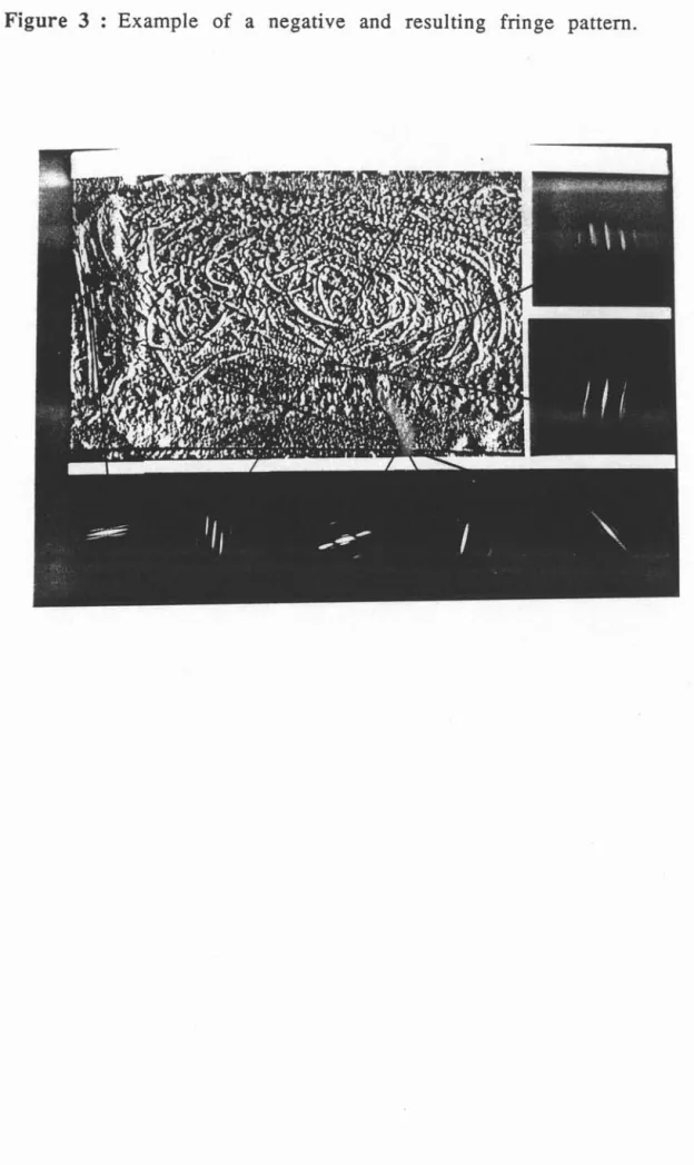
perpendicularly ta the moving wall. The laser is modulated using a chopper (or sector) model SR 540 from Stanford Research Systems Inc., providing pulses of light with adjustable frequency. The chopping frequency is dependent on the range of velocities present, which in tum depends on the imposed wall speed V and the spatial location within the cavity. In our experiments, the chopping frequency is varied from 10 to 60 Hz. In the technique, a negative is multiply exposed ; the total exposure time determines the numb~er of exposures taken on the same picture Le. the number of spots given by the same tracer. The exposure time used is also dependent on the cylinder speed of the experiment and on the spatial region of the flow that is ta be investigated, and the optimum time is determined by trial and error. Both velocimetry and flow visualization are accomplished by light scattered by seeding particles in the illuminated plane. The assumption in such techniques is that the seed particles follow the fluid without significant lag and do not alter the flow dynamics. The first requirement limits the particle size, the second limits the particle concentration. Spherical polystyrene particles of 200 J.1 m diameter have been used. As for the concentration, it is difficult to maintain it at a constant and known value due ta the fact that sorne fluid is flowing away of the cavity continuously. The particles number is diminishing with time, an injecting system is constructed to renew particles continuously. Under these conditions of low seeding concentration, the image pattern consists of sequence of superimposed particles images. This image is recorded by means of a camera on a high resolution film (Kodak Technical Pan 2415, ASA 125 with a resolution of 300 lines.pairs/mm). In velocimetry, the local fluid velocity is derived from the ratio of measured spacing between the images produced by the same tracer and the time between exposures or pulses of lighte The recorded image is a complicated random pattern. One of the methods of analysis is to produce Youngts fringes by Fourrier transform of the negative point by point. These fringes have an orientation perpendicular to the direction of the local displacement vector and a spacing inversely proportional to its magnitude. Figure 3 shows an example of a photograph and corresponding fringe patterns.
We can note that the use of such technique to determine local velocity imposes that the flow has a sufficiently two-dimensional nature, so that tracers stay in the light sheet during the total exposure time.
The procedure followed is first to position the cavity against the cylinder by fixing the cavity-cylinder distance in stable conditions (Le. with no leak at the cavity bottom part). Then, the cavity is filled with water and the entry flow rate .is adjusted to the exit one, in a way to maintain the liquid level h constant. The
particles~ used as tracers are introduced continuously in the bath. The cylinder is
set in' rotation at the chosen speed of the experiment. The desired data are taken when a steady-state is established which takes approximately 15 min after a change in conditions.
To . avoid hysteresis or ftmemoryft effects, the experimental sequences are accomplished by steps of increasing velocity.
-25-5
The cylinder surface state i.e. rugosity and chemical contact with the fluid, is considered constant aIl along this study.
III - RESJJLIS
, The cylinder speeds covered in this work ranged from 0,3 to 6 m- l , the liquid levels h from
la
-2 tola
-lm. The corresponding range of Re to Ca covered are given in Table 2. In addition to qualitative and quanti~ative details, the main result of this work is that we have discovered and identified three different flow regimes to which we have associated a specifie behavior of the liquid film at increasing constraints (h or V). For convenience, we will separate the discussion into three parts, dealing with each hydrodynamic behavior.3.1. The recirculating vortex
a - Bulk behavior
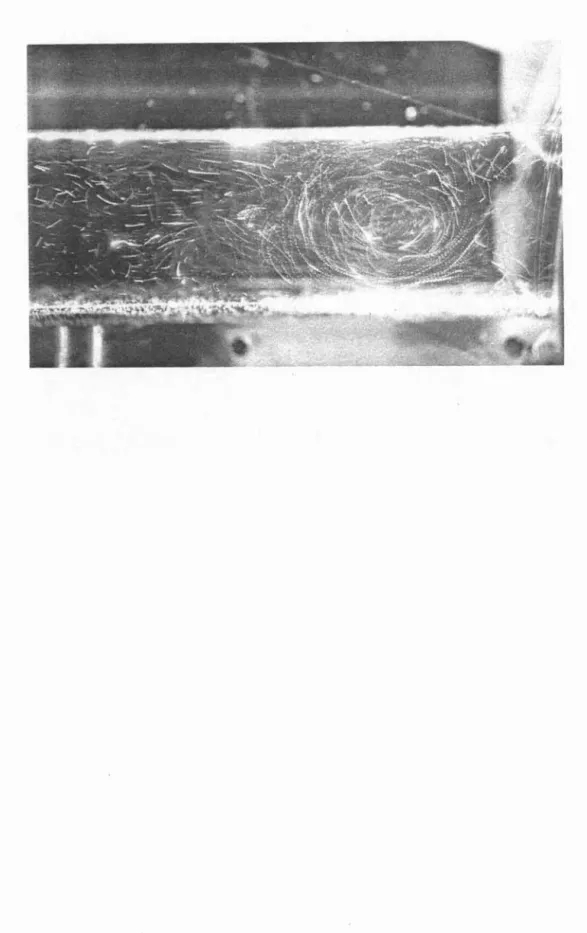
At low velocity V, the bulk flow shown on Figure 4 is similar to the recirculation flow driven by a lateral moving wall in a closed cavity. Rotation of the cylinder induces the formation of a recirculating vortex with a boundary layer along the moving wall. At the top meniscus, the boundary layer separates into two parts : one adhering to the vertical wall forms the film while the other one is flowing back to the rear under the free surface to constitute the recirculating vortex. Visualizations along the width show that in the central part of the cavity the fluid flow is essentially two-dimensional.
It . is of interest to note sorne characteristics specifie to this flow : the vortex seems to establish itself better in a cavity of higher A2 aspect ratio (~ 1). As speed V increases, the vortex center is shifted to the rear of the cavity, due to an increasing fluid velocity along the free surface. For a high fixed value of V, the vortex center is unsteady, its position is varying with time back and forth on an horizontal axis. Visualizations show the streamlines near the moving wall curve down at the bottom of the cavity and curve up in the upper part of the cavity.
b - Velocity profile
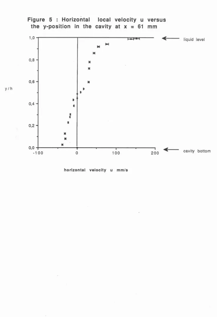
The local horizontal velocity is measured from each photograph along a vertical axis including the vortex center. Velocity profile obtained by interpolation of these data is presented Figure 5 in the case of the photograph of Figure 4. It shows features typical of recirculating flow namely a large free surface velocity and a core region of weak circulation.
c - Surface behavior
The horizontal surface of the fluid, the meniscus and the vertical film surface are observed visually. In this low speed region, a quantity of liquid is observed to flow back to the rear along the horizontal surface with an important velocity.
-26
6
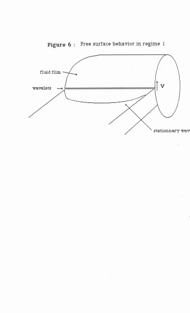
We notice on figure 6 the existence of a peculiar transverse lign' on the horizontal surface, corresponding ta a stationary wave which position varies with local surface velocity.
Small waves travel on the meniscus along the width (1 direction), whose wavelength is estimated to 10 mm.
The film surface on the vertical wall is smooth and stable.
3.2. The second regime : gravity fallback flow
This regime exists only for experiments done al value of h high enough for its appearance.
a - Volume hydrodynamics
The recirculating vortex of the first regime has disappeared. A boundary layer forms along the moving wall, aIl the fluid constituting it is dragged out of the bulk on the cylinder through the meniscus. Then, a part of it fall back in the bath by gravity and flow vertically in the volume along the ascending boundary layer to create a thin shear layer near the cylinder.
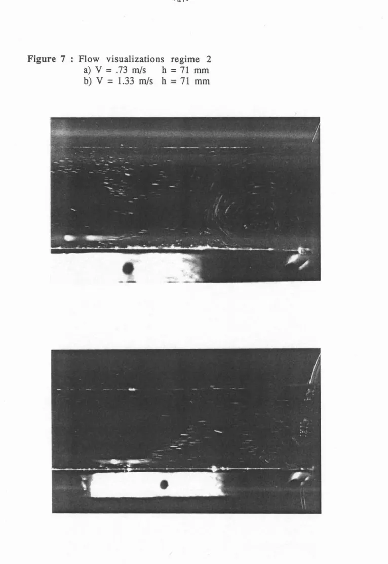
The bulk flow presents a small vortex confined in the bottom of the cavity near the moving walL It is rotating inversely to the cylinder since it is induced by the descending fluid from the film and the meniscus. At increasing speed, this vortex size diminishes as shawn on Figure 7.
Bulk flow far from the cylinder presents a regular, horizontal motion from the entry to the moving wall.
b - Velocity profiles
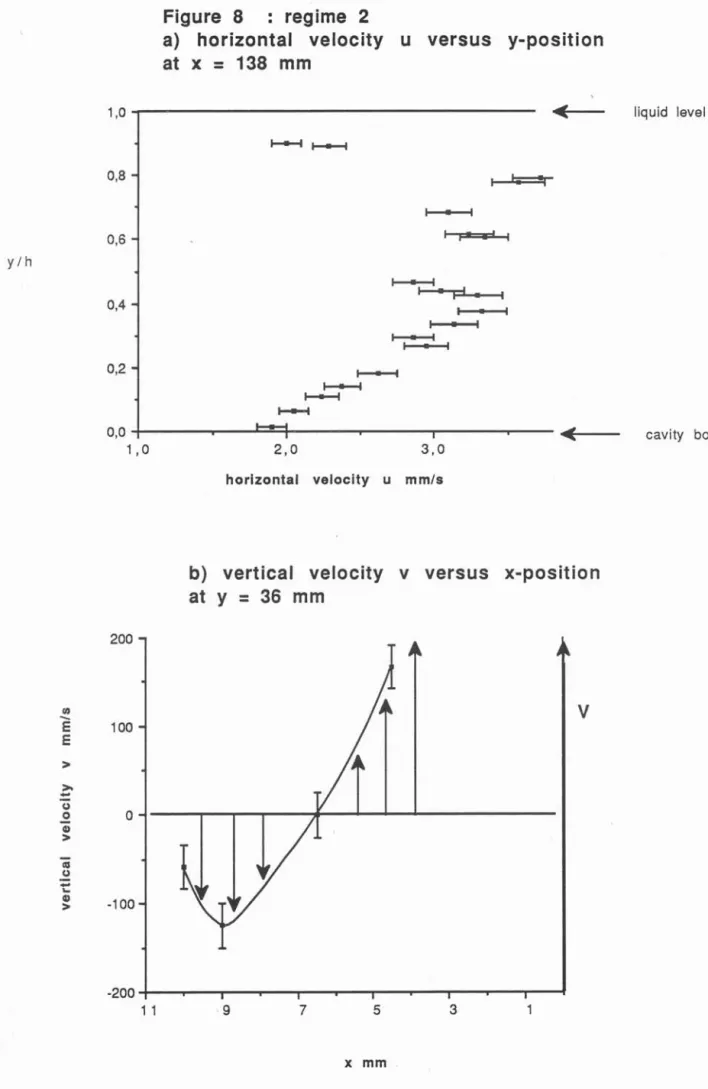
Vertical local velocities taken along a horizontal axis through the boundary layer Figure 8-a, shows the shear layer.
On Figure 8-b, horizontal velocities on a vertical axis taken far from the moving wall shows the regular bulk flow.
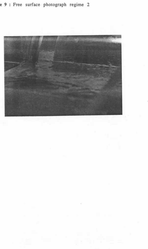
c - Surface behavior Figure 9
In this regime, a cloudy band appears just above the meniscus at the formation of the film dragged by the cylinder. The height of this band increases with the imposed speed : 5 mm for V
=
.9 m s-1 and 40 mm for V=
1.6m s-1 . The fluid flux is highly disturbed. The contact line at the meniscus is perturbed by waves of high amplitude which wavelength is estimated to 35 mm. These important surface perturbations, formed at the meniscus, propagate on the bath surface as waves.
-27-7
3.3 Boundary layer turbulence regime
For an imposed cylinder velocity above the critical value of 1.6 m s -1, the flow patterns show sorne irregular mixing in the flow and streamlines are not so clearly distinguished as those shown in figures 4 and 7. This suggests that flow field is not in the laminar regime.
a - Bulk flow
Figure 10 shows flow visualizations taken at three V values. The third regime differs from the two first ones in the way that it does not present any vortex.
We can observe that the flow is regular and laminar from the entry flow at the rear to the moving wall. The absence of volumic vortex allow us to note that the streamlines are highly downcurved in the lower part of the cavity next to the moving wall.
The singular aspect of this regime is the behavior observed in an area just under the meniscus. There, a highly perturbed zone is developing where 3D turbulences are observed in the boundary layer. This zone dissociates from the rest of the flow due to the random 3D motion of the illuminated tracers.
Photographs obtained at three velocities V, are presented on Figure 10. We can observe that at increasing cylinder speed, the turbulent zone is lengthened down along the moving wall, instabilities originate sooner in the boundary layer, and shortened along the free surface, the horizontal fluid velocity increasing pushes the turbulent zone against the wall. On the visualization Figure 10-c, obtained at V
=
3 m s·1 , beyond the general characteristics of the third regime, appears vibrations on the particles pathlines, with a small amplitude and a frequency of around 1Hz. The appearence area of these vibrations, first limited to the approach of the moving wall is increasing in the whole bath at increasing velocity.b -Velocity profiles
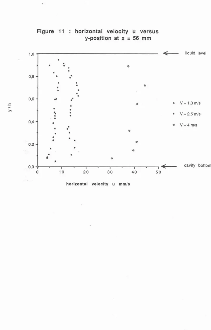
On Figure Il, we reported the velocity profiles obtained from horizontal local velocities in the bath at a given vertical axis for various values of V. They show that the fluid is flowing more rapidly near the bottom and the free surface and that the mean horizontal velocity increases with the imposed velocity.
c - Surface behavior
The process of gravity fallback has disappeared. The instabilities observed in the bulk manifest themselves first by the formation of small vortices (a few millimeters diameter) in the meniscus thickness.
At higher speed, the small vortices are replaced by violent disturbances visualized on Figure 12. These surface instabilities first intermittent and localized on small parts (2-3 cm) of the contact line, become then permanent and occupy the whole bath width l, producing a water film entirely perturbed.
8
. 3.4 - Existing do mains of the three regimes
At the observed three flow regimes we can attribute a limited domain in the parameter space (h,V) investigated in this study, at the other parameters fixed. The results are reported Figure 13 where each transition from one flow regime to another is extrapolated as a curve. Notice that the speed V is the determining parameter of the system, since each transition occurs at a critical value of V almost independently of the height h.
The regime 2 has a restricted domain inserted in the regime 1 domaine As' described previously in the protocol, the stability domains are determined at increasing values of the imposed wall velocity V between 2 experiments. However, no hysteresis has been revealed by proceeding al decreasing velocity. So, knowing the values of h and V chosen, it is DOW possible to predict the system
behavior using the map given in Figure 13.
3.5 • Flow rate measurements • Film thickness
The flow rate dragged out have been measured for four values of h, at increasing speed. The results are reported Figure 14 as average .. film thickness e versus V (at a c'onstant h).
The curve tendancy is surprising but tightly correlated with the system hydrodynamic behavioro In the first two regimes, as V increases, the mean thickness e increases ; then e presents a maximum value corresponding to the transition regime 1 - regime 3 and decreases with regime 3.
The transition 1-2, which appears only for values of h above 60 mm, is characterized by a change in the curve slope.
Notice that in the positive slope branch, corresponding to the regimes 1 and 2, the measured value of the film thickness· does not depend on the h parameter. Meanwhile, the maximum value of e which follows the transition 1-3 in the (h, V) parameter space increases with the liquid height h.
IV •
DISCJJSSIONWe propose in this part, to speculate on the mechanisms of the different observed instabilities. We focuse more specifically on the unexpected variation of the mean thickness with V and on its correlations with the system hydrodynamic.
4.1 • Drag out of liquid on fIat plates
As mentionned in the introduction, much study has been devoted to the thickness of films remaining on the surface of a solid withdrawn from a quiescent
liquido We propose here to compare the eXIstlng theories with the new
experimental data obtained with our system. These ones are very different from the experimental data cited in li terature, previous studies dealing wi th viscous liquids.
-
29-9
Formulation
o.'
the oroblemAt the position where the cylinder leaves the bath, the problem can be approximated to the continuous vertical withdrawal of a plane plate [3].
The process can be described conveniently by subdividing it into three regions (Figure 15) :
1. In the region weIl above the liquid level, the flow is parallei and the effect of liquid curvature is negligible.
2. The region of the dynamic meniscus. Here e changes with distance x.
3. This is the region close to the water Hne. Here the flow effects are less pronounced and the system can be described by the equation of capillary statics.
White et Tallmadge [1] and Tallmadge et Gutfinger [2] solved Navier-Stokes equations, in the case of a Iinear 2D theory, for the three regions. By using matching conditions between region 1 and 2, they showed that an asymptotic solution exists for small values of the capillary number :
According to this expression, the film thickness increases with the velocity as y2/3.
More recently, Esmail et al [4] and Magnin [5] tackled the same problem using a non linear 2D theory introducing inertial effects. Navier-Stokes equations are solved numerically in the assumption of lubrication theory and with the associated boundary conditions.
Results anal,)'sis
Experimental results and data obtained from theoretical studies are reported on Figure 16.
Theoretical data are smaller than experimental values. We observe a good agreement between the slope of the curve extrapolated from Tallmadge's linear analysis and the measured film thickness with Y variation.
However, we notice deviations with both analysis ; we can attribute them to the various approximations introduced in the analytical investigations. The following effects seem to be particularly important
- finite dimensions (width) of the container.
- important fluid flow in thë bath.
- validity of the lubrication theory at high capillary numbers.
assumption of a stagnation point at the transition region 1 - region 2.
steady-state flow in the film.
-30-10
Experiments have shown the existence of an important volumic fluid flow and that the film surface can be destabilized as visualized during regimes 2 and 3.
Despite these discrepancies, the existing theories give a reliable prediction of the (e-V) variation for low V values .
Film stabiliQ'
Descriptions of the surface in the regime 2 reveal that the dragged film is destabilized by a wave motion, waves velocity vector being perpendicular to the mean flow velocity direction. Few studies have been devoted to this phenomenon, beside the basic work of Levich [3] see for example Esmail et al [13] and Pommeau [ 1 4]. They give a critical value of Ca corresponding to the capillary waves apparition on the contact line :
Ca critical
=
1,472 Y -18/44 - 1,492 y-9/11wi th
1/3
Calculation for water leads to : y= 3008 and Cac~ 10-2
This calculated value of Cac corresponds to the working domain that we investigate here. This could explain the apparition of a wave regime on the contact line and on the film surface, perturbations which modify the (e- V)' curve evolution.
4.2 Turbulent regime
Bulk visualizations and surface observations of experiments done at high imposed velocity (regime 3) evidence that the boundary layer along the moving wall and the film issued from it cease to be in laminar motion. The system undergoes a transition to a turbulent flow which develops first in the boundary layer. In addition, this change in the flow behavior is accompanied by a sudden change .in the (e. V) curve slope, which becomes negative during the third regime (Figure 14).
These observations are, to our knowledge, unique in the sense that such behavior have never been observed before in the case of drainage of a film on a solid withdrawn from a bath.
Such experimental evidences are attributed to the apparition of a turbulent regime. According to Schlichting [15], transition from laminar to turbulent flow in a boundary layer along a wall becomes clearly discemible by a sudden and large increase in the boundary layer thckness and in the shearing stress near the
wall. The critical Reynolds number Rex based on the current length x,.
-31-I l
Rex critique
=
CV
X)critical=
3,2 x 10⁵v
Transposition of this value in our case and a current distance h of 10 cm leads to a critical velocity value of 3.2 m s-l. This critical value is of the arder of magnitude of the observed v~lue of the transition. The existence of a waving free surface, the curvature of the' wall and its relative roughness could be sufficient distrubances to induce turbulence earlier.
Apparition of a turbulent boundary layer and its development along the wall in the regime 3 allows us ta explain the decreasing tendancy of e at increasing velocity Y. In this regime, the gravity fallback have ceased, sa we can suppose that the flow rate in the film is equal to the flow rate in the boundary layer at the height h ; (Le. the fluid in the b.l. is entirely dragged out to form the fi lm).
In a laminar flow, ô the boundary layer thckness decreases as y-1/2 in a turbulent flow, ôt decreases as Y -0,2.
The decreasing branch of the (e- Y) curve calculated from several experiments shows a variation as y(-0,32).
This value permits us to conclude that the third regime corresponds to a transient state where turbulent flow is not completely instaled.
y -
CONCLUSIONSFrom a variety of qualitative and quantitative observations and
measurements we are able to conclude that for the range of parameters studied, the drainage of a film adhering to a solid moving through a liquid volume presents a sequence of three hydrodynamic regimes.
At increasing constraint, the system undergoes a transItIon from a laminar recirculating flow similar to a cavity circulation driven by the motion of one of the walls to a flow perturbed by a gravity fallback process. Then, at higher constraint, a third regime appears which shows a regular flow supplying a turbulent boundary layer. Each volume circulation is correlated to a specifie surface behavior an increase of constraint inducing a more perturbed free surface.
Unexpected varIatIon of the film mean thickness with wall velocity is found and explained. At low velocity, the experimental data are in agreement with the extrapolation of a linear theory of drainage of a thi.n film on an ascending plate. At high velocity~ measurements and observations agree with the apparition of a turbulent boundary layer along the moving wall. However, the whole system behavior could be explained only with a complete analytical study' including the coupled phenomena : drainage - bulkflow.
·32-12
REFERENCES
[1] WHITE D.A. and TALLMADGE J.A.
Theory of drag out of liquid on flat plates Chem. Engineering Science, 1965, 2.Q, p 33-37.
[2] TALLMADGE J.A. and GUTFINGER Co
Films of Non-Newtonian fluids adhering to faIt plates A.I.Ch.E. Journal, 1965,
il,
3, p. 403-412.[3] LEVICH V.G.
Physicochemical hydrodynamics - Chap 12. Prentice Hall New-York, 1962.
[4] ESMAIL M.N. et HUMMEL R.L.
Chem. Engineering Science, 1979,
.3±,
p 125-129.[5] MAGNIN A.
Etude expérimentale et théorique de la dépose d'ensimage au rouleau sur des fibres textiles.
Thèse INPG, 1983, Grenoble.
[6] DERYAGIN B.V. and LEVICH V.G.
Film coating theory. Focal Press. New-York, 1964.
[7] BATCHELOR O.K.
On steady laminar flow with closed streamlines at large Reynolds numbers. J. Fluid Mech., 1956,
l,
177.[8] BUROGRAF O.R.
Analytical and numerical studies of the structure of steady separated flows. J. Fluids Mech., 1966, 24, 1, 113.
[9] PAN F. and ACRIVOS A.
Steady flows in rectangular cavltles J. Fluid Mech, 1967,
ll,
4, 643-655. [10] LüURENCO L. and KROTHAPALLI A.The role of photographie parameters in Laser Speckle or particle image displacement velocimetry
Experiments in Fluids, 1987,
i,
29-32. [11] LANDRETH C.C., ADRIAN R.J. and C.S. YAODouble pulsed particle image velocimeter with directional resolution for complex flows.
Experiments in Fluids, 1988,
6.,
119-128.[12] Lambertus HESSELINK
Digital Image Processing in Flow Vizualisation Ann. Rev. Fluid Mech., 1988, 2.Q, 421-85.
[13] ESMAIL M.N., HUMMEL R.L., et SMITH J.W. Phys. Fluids, 1975,
li,
508.-13"
13
[14] POM~AUY.
Sorne current problems in capillary phenornena : Contact angle hysteretis and contact line motion.
PhysicoChemical Hydrodynamics, 1985, ~, 5/6, 727-730.
(15] SCHLICHTING H.
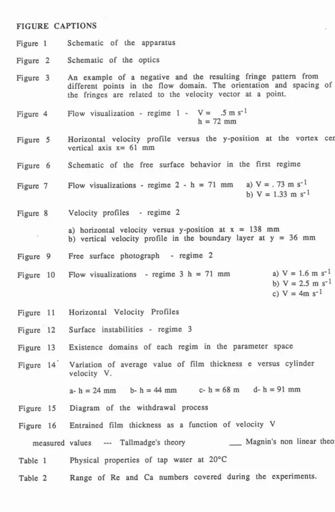
-34-· 14 FIGURE CAPTIONS Figure 1 Figure 2 Figure 3 Figure 4 Figure 5 Figure 6 Figure 7 Figure 8 Figure 9
Schematic of the apparatus
Schematic of the optics
An example of a negative and the resulting fringe pattern from different points in the flow domaine The orientation and spacing of the fringes are related ta the velocity vector at a point.
Flow visualization - regime 1 - V
=
.5 m s-1 h=
72 mmHorizontal velocity profile versus the y-position at the vortex center vertical axis x= 61 mm
Schematic of the free surface behavior in the first regime
Flow visualizations - regime 2 - h = 71 mm a) V = .73 m s-1 b) V = 1.33 m s-1 Velocity profiles - regime 2
a) horizontal velocity versus y-position at x
=
138 mmb) vertical velocity profile in the boundary layer at y
=
36 mm Free surface photograph - regime 2Figure 10 Flow visualizations - regime 3 h
=
71 mm a) V=
1.6 m s-1 b) V = 2.5 m s-1 c) V = 4m s-1 Figure Il Horizontal Velocity ProfilesFigure 12 Surface instabilities - regime 3
Figure 13 Existence domains of each regim in the parameter space
Figure 14 Variation of average value of film thickness e versus cylinder velocity V.
a- h = 24 mm b- h= 44mm c- h
=
68 m d- h=
91 mm Figure 15Figure 16
Diagram of the withdrawal process
Entrained film thickness as a function of velocity V
measured values --- Tallmadge's theory _ Magnin's non linear theory
Table 1
Table 2
Physical properties of tap water at 20°C
-35-Figure 1
honeycomb gridbarrage
l
1
t "2Uater supply "Water exit cy1.inder balance-
36-Figure
2
light sheet cavity seeded lenses chopper 5W Argon laser camera position-~
-1~
--39-Figure
5
.
.
Horizontal
local velocity u versus
the y-position in the cavity at
x
=
61
mm
1,0 ~
C
liquid level t-4 III lit 0,8 -III III 0,6 -•
y/h Il 1 Il 0,4-•
1•
•
0,2 •..
•
III 0,0 1 1C
cavity bottom -1 00 0 100 200 horizontal. velocity u mm/s
..---~---;---;---~----~~-
-40-Figure 6:
Free surface behavior in regime 1
vavelets
..
Figure 7 :
Flow visualizations regime
2
a) V
=
.73
mis
h
=
71 mm
b) V
=
1.33
mis
h
=
71 mm
-42-Figure 8
regime 2
a)
horizontal velocity u versus y-position
at x
=
138
mm
1,0 . . . . - - - liquid level 0,8 1 ...,.. 1 • 1 0,6 1 i , 1 y/h 0,4...-...
1 • 1 ' . 1 1 • 1 1 • 1...-...
a---I 0,2 2,0 0,0-+---.,...--...-+----....---....----.---- ..
~~-1 ,0 cavity bottom . horizontal velocity u mm/sb)
vertical velocity v versus x-position
at
y
=
36 mm
5· 7 ·9 200 -200-+--...--....-...--....-...-..,.--~-,...,,.,,._-,.-__r 1 1 enV
---
E 100 E >>-=
(,) 0 0 Q) > -; (,)...
'-Q) -100 > x mm .-/.JIJ
Figure 10
Flow
visualizations regime
3
a)
V
=
1.6
mis
h
=
71
mmb) V
=
2.5
mis
h
=
71
mm
-45-Figure
11
horizontal velocity u versus
y-position at x
=
56 mm
1,0<
liquid level•
•
a• •
•
•
0~8 a•
•
..
•
•
..
..
•
•
•
0,6 ~•
•
•
V=1,3
mIs ..c•
a•
>...
•
•
V=2,5
mIs..
•
..
0,4..
~ V=4
mIs•
..
•
@•
•
•
•
..
•
~ 0,2..
•
<) a•
1•
0,0<
cavity bottom 0 1 0 20 30 40 50 horizontal velocity u mm/s-47
Figure
13
100-p---.
5 4 3 2 20 ...--.r---...-...-.~-_P___...-...____.,..___._~o
80 E E .c 600
...
.c C)0)
Qi .c 40 velocity V mis
-48-Figure 14 a
0,28 h=24mm E 0,23 E en en Q) c: ~ 0,18 ~ .c...
E ;: 0,13 3 6 5 4 3 2 0, 08-+--:or---.--...-....-~-...--.-....--.--..---..---.1o
velocity V mIsFigure 14 b
0,28 h=44 mm E 0,24 E fi) fi) Q) c: ~ ~ 0,20 .c...
E ;: 0,16 3 0,12 0 2 3 4 5 6 velocity V mIs
-49-Figure 14
c
0,35 h=68 mm 0,30 E E U) 0,25 fi) Q) c ~ ~ .c 0,20...
E ;: 0,15 2 3 0,10 0 2 3 4 5 6 velocity V mIsFigure 14 d
0,4 . . . - - - . h=91 mm velocity mIs 5 4 3 3 2 2o
E 0,3 E U) fi) Q) c ~ ~ .c...
E 0,2 ;:v
-10-Figure 15
region 1...- ...
~y region 2 region 3~
non linear theory 5]-Figure
16
0,3 A A A/
0,2 A/ '
E E A / ' en A/
en Q) c/
~ ~ .r;./
..
E ;: 0,1 ~...--experimentextrapolated linear theory'
2
0,0- + - - - - -...- - - . . . - - - -...- - - 1
°
1,6 2 4 6 7.3 10-2 4 0.022 0.027 0.055 0.082
o
32000 40000 80000 120000o
80000 100000 200000 300000o
128000 160000 320000 480000 -52 table 1 E> J..L v kg m- 3 N s m- 1 m 2 s-1 1000 10-3 10-6 table 2 V ms- 1 0,2 O,S 1 Ca 0.003 0.007 0.01 Re (h=20~m) 4000 10000 2000 Re (h=SO~m) 10000 2S000 SOOO Re (h=80~m) 16000 40000 8000-5J'
CONVECTION FORCEE EN PRESENCE D'UNE SURFACE LIBRE VISUALISATION et VELOCIMETRIE LASER
Pr GILLON; P. RIVAT et Y. FAUTRELLE
Laboratoire MADYLAM, ENSHMG, B.P. 95 38402 SAINT MARTIN D'HERES CEDEX.
Compte rendu du Ilème Congrès Francophone de Vélocimétrie Laser, Meudon, 25-27 septembre 1990
RESUME
L'étude expérimentale des mouvements convectifs engendrés dans une cavité ouverte par une paroi défilante verticale est effectuée par PlV.
A vitesse croissante, une suite de trois reglmes hydrodynamiques est observée : le système passe d'un écoulement type recirculation en cavité à un écoulement à couche limite cisaillée pour présenter ensuite une circulation régulière de fluide alimentant une couche limite turbulente.
INTRODUCTION
Nous présentons une étude expérimentale de la circulation d'un fluide contenu dans une cavité ouverte en présence d'une paroi défilante. Le paramètre variable étudié ici est la vitesse U de la paroi. Les visualisations du mouvement et la ." ':\. vélocimétrie' sont obtenues à l'aide d'une technique laser. La Vélocimétrie par Image de Particules (PlV) permet l'évaluation qualitative et la mesure simultanée de l'ensemble des vitesses locales d'un plan de l'écoulement.
INSTALLATION EXPERIMENTALE (figure 1)
L'écoulement à étudier est établi dans une cavité ouverte, de section rectangulaire 650 x 400 mm2, à fond incliné dont l'extrémité est en contact avec la paroi défilante. Afin de permettre les visualisations, l'ensemble cavité-paroi mobile est en Plexiglass. Le liquide utilisé, l'eau, est introduit dans la cavité en continu par une alimentation ; un déversoir à l'arrière permet de maintenir le niveau liquide constant.
La cavité au contact de la plaque mobile, est alimentée en eau jusqu'au niveau choisi, la paroi est alors mise en mouvement à une vitesse U contrôlée entraînant par drainage un film liquide dont l'épaisseur peut être mesurée.
L'étude expérimentale de ce système repose essentiellement sur la
visualisation et la vélocimétrie de l'écoulement.
VELOCIMETRIE PAR IMAGE DE PARTICULE
Principe
La Vélocimétrie par Image de Particules (VIP) a été développée pour déterminer des valeurs quantitatives de vitesses locales dans des écoulements fluides, voir par exemple les travaux de Laurenco et Krothapalli [ 1 ] (1987), Adrian [ 2 ] (1986) et la revue de Hesselink [ 3 ] (1988).
Le faisceau d'un laser Argon 5 W à 514 nm traverse un système de lentilles pour former une tranche lumineuse. Cette tranche laser vient illuminer une section choisie de la cavité perpendiculairement à la paroi défilante. Le faisceau laser est modulé par un secteur tournant, produisant ainsi un éclairement' pulsé à
fréquence ajustable. Dans cette technique, le négatif subit une exposition multiple; le temps d'exposition total détermine le nombre de spots donnés par un même traceur. Le temps d'exposition utilisé, dépend de l'ordre de grandeur des vitesses présentes et de la région spatiale à étudier.
par
Visualisation et vélocimétrie de la la lumière renvoyée par les particules
circulation sont situées dans le
obtenues simultanément plan illuminé.
i
milieu liquide +particules
lentilles
secteur tournant
laser argon haute puissance
Figure 1
Schéma de la technique visualisation vélocimétrie
position de l'observateur
L'hypothèse dans de telles techniques est que les particules utilisées comme traceurs, suivent le fluide sans retard significatif et n'altèrent pas la dynamique de l'écoulement. La premlere assertion limite la taille des particules, la seconde limite leur concentration. Des particules sphériques de polystyrène de 200 (lm de diamètre ont été utilisées.
La concentration des particules est dans notre cas difficile constante et connue puisque l'-écoulement entraîne une quantité de l'extérieur de la cavité, le nombre de particules présentes diminue temps et est renouvelé par ajouts successifs.
à maintenir particules à au cours du