A study on the scale effects of propulsive characteristics of podded propulsors

(1)

Publisher’s version / Version de l'éditeur:

Vous avez des questions? Nous pouvons vous aider. Pour communiquer directement avec un auteur, consultez la Questions? Contact the NRC Publications Archive team at

PublicationsArchive-ArchivesPublications@nrc-cnrc.gc.ca. If you wish to email the authors directly, please see the first page of the publication for their contact information.

https://publications-cnrc.canada.ca/fra/droits

L’accès à ce site Web et l’utilisation de son contenu sont assujettis aux conditions présentées dans le site

LISEZ CES CONDITIONS ATTENTIVEMENT AVANT D’UTILISER CE SITE WEB.

Student Report (National Research Council of Canada. Institute for Ocean Technology); no. SR-2006-18, 2006

READ THESE TERMS AND CONDITIONS CAREFULLY BEFORE USING THIS WEBSITE.

https://nrc-publications.canada.ca/eng/copyright

NRC Publications Archive Record / Notice des Archives des publications du CNRC :

https://nrc-publications.canada.ca/eng/view/object/?id=e9dcc87b-9590-4a9e-be23-92083d54d5b7 https://publications-cnrc.canada.ca/fra/voir/objet/?id=e9dcc87b-9590-4a9e-be23-92083d54d5b7 For the publisher’s version, please access the DOI link below./ Pour consulter la version de l’éditeur, utilisez le lien DOI ci-dessous.

https://doi.org/10.4224/8895016

Access and use of this website and the material on it are subject to the Terms and Conditions set forth at A study on the scale effects of propulsive characteristics of podded propulsors

(2)

REPORT SECURITY CLASSIFICATION

Unclassified

DISTRIBUTION

Unlimited

TITLE

A STUDY ON THE SCALE EFFECTS OF PROPULSIVE CHARACTERISTICS OF PODDED PROPULSORS

AUTHOR(S)

Stephen Lane

CORPORATE AUTHOR(S)/PERFORMING AGENCY(S)

Institute for Ocean Technology, National Research Council, St. John’s, NL

PUBLICATION

N/A

SPONSORING AGENCY(S)

Institute for Ocean Technology, National Research Council, St. John’s, NL

IMD PROJECT NUMBER

42_2085_16

NRC FILE NUMBER KEY WORDS

Podded, Propeller, Propulsors, Azimuthing

PAGES v, 33, App. A-H FIGS. 24 TABLES 22 SUMMARY

The following is a report detailing the procedure, analysis, and results of seven sets of tests conducted on podded propellers. The tests were conducted on either a single pod or dual pods running along side one another. Two sets of tests were conducted on a propeller of 270mm while the remainder were on a prop of 200mm. Two of the cases were numerical.

Not much is known about the performance characteristics of podded propellers to this date. This is reason behind the current study. With the data already collected along with future tests planned researchers will gain valuable knowledge about podded propellers and will be able to engineer future pods more efficiently and effectively.

ADDRESS National Research Council

Institute for Ocean Technology Arctic Avenue, P. O. Box 12093 St. John's, NL A1B 3T5

(3)

National Research Council Conseil national de recherches

Canada Canada

Institute for Ocean Institut des technologies

Technology océaniques

A STUDY ON THE SCALE EFFECTS OF PROPULSIVE

CHARACTERISTICS OF PODDED PROPULSORS

SR-2006-18

Stephen Lane

(4)

TABLE OF CONTENTS

List of Tables ...iii

List of Figures...iv

List of Abbreviations ... v

1.0 INTRODUCTION ... 1

2.0 DESCRIPTION OF THE MUN-NRC-NSERC POD MODEL ... 1

3.0 DESCRIPTION OF FACILITIES... 2

3.1 NRC-IOT Ice Tank... 2

3.2 MUN Towing tank ... 3

4.0 DESCRIPTION OF INSTRUMENTATION... 4

4.1 Experimental Apparatus ... 4

4.1.1 NRC-IOT dynamometer ... 4

4.1.2 NSERC-NRC pod dynamometer (or MUN dynamometer) ... 5

4.2 Opens Boat ... 7

4.3 Data Acquisition System (DAS) ... 8

4.3.1 NRC-IOT tests... 8 4.3.2 MUN tests... 9 5.0 DESCRIPTION OF CASES... 9 5.1 Case 1 ... 9 5.2 Case 2 ... 11 5.3 Case 3 ... 11 5.4 Case 4 (a and b) ... 12 5.5 Case 5 (a and b) ... 13 5.6 Case 6 ... 17 5.7 Case 7 ... 17 6.0 DESCRIPTION OF EXPERIMENTS ... 19

6.1 Reynolds Number Effect Tests... 19

6.2 Air Friction Tests... 20

6.3 Bollard Runs ... 20

6.4 Opens Tests (0 degree azimuth) ... 20

7.0 DESCRIPTION OF DATA ANALYSIS ... 21

7.1 Interpreting the Raw Data (MUN Towing Tank Tests) ... 21

7.2 Interpreting the Raw Data (NRC-IOT Ice Tank Tests) ... 22

8.0 CALIBRATIONS... 23

8.1 Global Dynamometer ... 24

8.2 Thrust and Torque Load Cells ... 25

9.0 RESULTS AND DISCUSSION... 26

10.0 RECOMMENDATIONS AND CONCLUSIONS... 32

11.0 ACKNOWLEDGMENTS... 32

(5)

APPENDIX A: Calibration Data for Global Dynamometer

APPENDIX B: Calibration Data for Thrust and Torque Load Cells

APPENDIX C: Data Acquisition System Channel Set-up for NRC-IOT Tests APPENDIX D: Results for Case One

APPENDIX E: Results for Case Three APPENDIX F: Results for Case Four APPENDIX G: Results for Case Five APPENDIX H: Results for Case Seven

(6)

LIST OF TABLES

Table 1: Geometric particulars of the pod-strut model ... 1

Table 2: General test plan for Reynolds Effects Tests ... 9

Table 3: General test plan for Air Friction Tests... 9

Table 4: General test plan for Bollards Tests ... 10

Table 5: General test plan for Open Tests ... 10

Table 6: General test plan for Oblique Flow Tests... 10

Table 7: General test pan for Third Quadrant Tests ... 10

Table 9: General test plan for Bollard Runs... 11

Table 10: General test plan for Opens Tests ... 12

Table 13: General test plan for Bollards Tests ... 14

Table 14: General test plan for Open Tests ... 15

Table 16: General test plan for Dynamic Tests ... 17

Table 18: General test plan for Bollard Runs... 18

Table 21: Data Reduction Equations used in analysis... 21

(7)

LIST OF FIGURES

Figure 1: Geometric Parameters... 2

Figure 2: NRC-IOT Ice Tank schematic ... 3

Figure 3: MUN Towing Tank schematic... 3

Figure 4: TDC Podded Props – General Arrangement... 4

Figure 5: 6-Component Balance... 5

Figure 6: NSERC-NRC Pod Dynamometer System ... 6

Figure 7: Global dynamometer looking from below... 6

Figure 8: Side view of system ... 7

Figure 9: Round Opens Boat ... 7

Figure 10: DAS set-up used for calibrations ... 8

Figure 11: Typical plot of rps and Carriage Velocity for one run down the tank ... 22

Figure 12: Typical plot of rps and Carriage Velocity for one run down the tank ... 23

Figure 13: Positive coordinate directions in 3-D space... 24

Figure 14: Photo showing how torque can be induced on the system... 25

Figure 15: Positive thrust and torque directions during calibrations... 25

Figure 16: Comparison of KT_prop versus J ... 26

Figure 17: Comparison of η_prop versus J... 27

Figure 18: Comparison of KT_unit versus J... 27

Figure 19: Comparison of η_unit versus J... 28

Figure 20: Comparison of KT_pod versus J ... 28

Figure 21: Comparison of η_pod versus J ... 29

Figure 22: Comparison of 10KQ versus J ... 29

Figure 23: Comparison of KT_side versus J... 31

(8)

LIST OF ABBREVIATIONS

D Diameter (Propeller) DAS Data Acquisition System

deg Degree(s)

EAR Expanded Area Ratio

Hz Hertz

ITTC International Towing tank Conference IOT Institute for Ocean Technology

J Advance Coefficient

KQ Torque Coefficient KT Thrust Coefficient m Metre(s)

mm Millimetre(s)

m/s(ec) Metres per Second n Shaft Rotational Speed

NRC National Research Council Canada

NSERC Natural Sciences and Engineering Research Council of Canada MUN Memorial University of Newfoundland

P/D Pitch-Diameter Ratio Q Torque

Rn Reynolds Number RPS Revolutions per Second T Thrust

V Speed (of advance)

η Open Water Efficiency

ν Kinematic Viscosity

(9)

1.0 INTRODUCTION

Podded propellers were introduced to the marine industry just over a decade ago and have since become a popular main propulsion system for ships. This is due to their better hydrodynamic characteristics than conventional propeller-rudder systems.

A podded propeller consists of a motor inside of a pod and a propeller(s) connected to the drive shaft at one or both end(s) of the shaft. The unit is connected to the vessel via a strut, which allows the whole system to rotate 360 degrees around the vertical, or z-axis. This allows for the thrust to be directed anywhere in a 360 degree compass, which gives far superior manoeuvring capabilities. The rapid adoption of podded propellers by the industry has outpaced the understanding of their performance. This lack of knowledge has

translated into problems in practice, including propeller and bearing damage as well as vibration during manoeuvring.

The purpose of this study is to increase the understanding of podded propeller performance. NRC could also use these tests as a solid base on which further testing could be completed.

2.0 DESCRIPTION OF THE MUN-NRC-NSERC POD MODEL

The experiments conducted were on either a single podded propeller or two podded

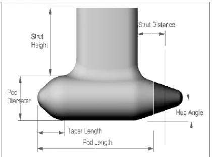
propellers operating simultaneously. Two of the cases used a propeller of 270mm diameter, while the remainder used a propeller of 200mm diameter. The arrangement and diameter of propellers are given in the section DESCRIPTION OF CASES for each particular case. All cases used a propeller that was four bladed, had a pitch-diameter ratio (P/D) of 1.0, and an expanded area ration (EAR) of 0.6. The geometric particulars of the pod are given below in Table 1. The values for the model propulsor were selected to provide an average representation of in-service, full-scale single screw podded propulsor. The geometric particulars of the pod-strut model were defined using the parameters depicted in Figure 1.1

Experimental Dimensions of Model Pods

Pod

mm Propeller Diameter, DProp 270 or 200

Pod Diameter, DPod 139

Pod Length, LPod 410

Strut Height, SHeight 300

Strut Chord Length 225

Strut Distance, SDist 100

Strut Width 60

Fore Taper Length 85

Fore Taper Angle 15o

Aft Taper Length 110

Aft Taper Angle 25o

(10)

Figure 1: Geometric Parameters

3.0 DESCRIPTION OF FACILITIES

Several of the test cases took place at the NRC-IOT Ice Tank, while one of the test cases studied took place at the MUN Towing Tank. The flowing sub-sections describe the two Tanks that the tests were performed in.

3.1 NRC-IOT Ice Tank

The NRC-IOT ice tank is 90m long, 12m wide and 3m deep. The ice tank is equipped with a towing carriage that is capable of velocities from 0.1 – 4.0m/s. The control room is thermally insulated and houses the computer equipment for the drive control and the instrumentation racks for the model test transducers. The tank can accommodate models from 2-12m in length; and is equipped with force measurement, strain gauge load cells, model motions, accelerometer arrays, along with other instrumentation; all of which allow for various types of tests to be completed in the tank.2

(11)

Figure 2: NRC-IOT Ice Tank schematic

3.2 MUN Towing tank

The towing tank facility at MUN has a length of 58m, is 4.5m wide, and a water depth of 2.2m. The tank is equipped with a towing carriage with a maximum towing speed of 5.0m/sec. The tank is equipped with a hydraulically operated wave maker, vertical mesh beaches, precision dynamometer, a 16 channel data acquisition system, along with other instrumentation; all of which allows for various types of testing to be competed at the facility.3

(12)

4.0 DESCRIPTION OF INSTRUMENTATION 4.1 Experimental Apparatus

As in the previous section, this section will also contain a description of the experimental apparatus used at the NRC-IOT Ice Tank as well as the MUN Towing Tank.

4.1.1 NRC-IOT dynamometer

The set-up shown below in Figure 3 was used for this set of experiments. The system has the ability to measure the propeller and pods forces and moments. It was used to measure unit thrust (Tunit), propeller thrust at hub end (Tprop), propeller thrust at pod end (Tpod),

propeller torque (Q), as well as forces in the three coordinate directions.3 The unit thrust is of particular interest, as it used for powering predictions for podded propellers. The unit thrust is the net available thrust available for propelling the ship. It not only includes the thrust of the propeller, but also the drag and other hydrodynamic forces acting on the pod-strut body.

The design includes an instrumented propeller hub, a custom mitre gearbox, an azimuth drive system, propeller drive system, a hull mounting and seal assembly, and a 6-component balance for measuring global loads on the pod.4

(13)

Figure 5: 6-Component Balance

4.1.2 NSERC-NRC pod dynamometer (or MUN dynamometer)

The NSERC-NRC pod dynamometer system, custom designed, was used during the experiments. The system has the ability to measure the propeller and pods forces and moments. It was used to measure unit thrust (Tunit), propeller thrust at hub end (Tprop),

propeller thrust at pod end (Tpod), propeller torque (Q), as well as forces in the three

coordinate directions.3 The unit thrust is of particular interest, as it used for powering predictions for podded propellers. The unit thrust is the net available thrust available for propelling the ship. It not only includes the thrust of the propeller, but also the drag and other hydrodynamic forces acting on the pod-strut body. The water temperature, carriage speed (V), and the rotational speed of the propeller (n) were also measured.

As can be seen below in Figure 3, the unit consists of two major components. The first part is the pod dynamometer, which measures the thrust and torque of the propeller at the propeller shaft. The second part of the unit is the global dynamometer, which measures the unit forces in the three coordinate directions at a location above the propeller boat. Also, a boat shaped body called a wave shroud was attached to the frame of the test equipment and placed just above the water surface. Further details of the experimental apparatus can be found in MacNeill et al. (2004).5

(14)

Figure 6: NSERC-NRC Pod Dynamometer System

(15)

Figure 8: Side view of system

4.2 Opens Boat

For the experiments conducted in the NRC-IOT Ice Tank an opens boat was constructed out of plywood, foam and glass. The opens boat floor was provided with slots that the pod drives fit into to allow the distance between the drives to be varied from as close as the drives could safely be run together to 3 times the width spacing of the pods.4

(16)

4.3 Data Acquisition System (DAS) 4.3.1 NRC-IOT tests

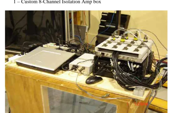
The Data Acquisition System (DAS) for this project is custom built with IOTech gear and RS232 data from the U500 controller. The system components were chosen to allow for the system to be placed into a free running model. The data was collected through a total of 26 channels; a detailed outline of the channel set-up is in Appendix C. The system

consisted of the following:

- 1 - Panasonic CF-51 Laptop, PC4026, S/N - 1 – Panasonic Docking Station

- 1 – D-Link DI-624 Wireless Router - 1 - IOTech Daqbook 2001, S/N 802671

- 2 - IOTech DBK 43A, 8 Channel Stain Gage Modules - 1 – Custom 16 Channel DBK 43A to 10 Pin breakout box - 2 - IOTech DBK 45, 4-Channel SSH and Low-Pass Filter Cards - 1 – IOTech DBK 10, Expansion Chassis

- 1 – Custom 8-Channel Isolation Amp box

(17)

4.3.2 MUN tests

The data for each of the test conditions was collected through 13 channels (three channels for propeller and pod thrusts and torque, two channels for shell drag, six channels for global loads, one channel for propeller rotational speed and one channel for carriage speed). The voltage data outputs for the tests were collected using an IOTech Daqbook data acquisition system (Daqbook 2000) connected to a computer running DaqView software. For these tests, the data were collected with a sampling rate of 59Hz. The raw data was collected in .txt format and post processed using Microsoft Excel. For each test run, data was collected for at least 10 second when the propeller run at very low rps (0.5 or less). Then the test data was collected following a standard procedure. The data collected at low rps was used to tare the test value. In this way the friction correction for thrust and torque was avoided.

5.0 DESCRIPTION OF CASES

As stated above, there were a total of seven sets of tests conducted. This section is intended to give a brief explanation of each case and the tests that were performed for each set of tests. A general test plan will be provided in each sub-section for each case.

5.1 Case 1

The tests were performed in the MUN Towing Tank in January 2005. The experiments conducted were on a single podded propeller with a diameter of 270mm. The following is a list of the types of experiments conducted: Reynolds Number Effects Tests, Air Friction and Bollard Runs, Opens Tests (0 deg azimuth), Oblique Flow Tests, and Third Quadrant Runs.

Reynolds Number Effects

Mode Pull Mode

RPS 8, 9, 10, 11, 12, 13, 14

Carriage Velocity (m/s)

1.728, 1.944, 2.16, 1.944, 2.187, 2.43, 2.16, 2.43, 2.7, 2.376, 2.673, 2.97, 2.592, 2.916, 3.24, 2.808, 3.159, 3.51, 3.024, 3.402, 3.78

Azimuth Angle (deg) 0

Table 2: General test plan for Reynolds Effects Tests

Air Friction Tests

Mode Pull Mode

RPS 1,2 (in both positive and negative directions)

Carriage Velocity (m/s) 0

(18)

Bollard Runs

Mode Pull Mode

RPS -11 to 10

Table 4: General test plan for Bollards Tests

Opens Tests

Mode Pull Mode

RPS 12

Carriage Velocity (m/s) 0.324, 0.648, 0.972, 1.296, 1.62, 1.944, 2.268, 2.592, 2.916, 3.24, 3.564

Table 5: General test plan for Open Tests

Oblique Flow Tests

Mode Pull Mode

RPS 12

Run #1

Carriage Velocity (m/s) 2.268, 1.62, 0.324, 3.24, 0.648, 0.972, 2.592, 1.944, 3.564, 1.296, 2.916, 4.0

Azimuth Angle (deg) -9

Run #2

Carriage Velocity (m/s) -1.62, -1.296, -0.324, -0.648, -0.972, -1.944

Azimuth Angle (deg) -9

Run #3

Carriage Velocity (m/s) 2.268, 1.62, 0.324, 3.24, 0.648, 0.972, 2.592, 1.944, 3.564, 1.296, 2.916, 4.0

Run #4

Carriage Velocity (m/s) -1.62, -1.296, -0.972, -1.944, -1.05

Table 6: General test plan for Oblique Flow Tests

Third Quadrant Tests

Mode Pull Mode

RPS 12

Carriage Velocity (m/s) 0.324, 0.648, 0.972, 1.296, 1.62, 1.944

(19)

5.2 Case 2

This is the numerical results of the same set-up as case 1; and was completed on Oct 24/04. They were computed for a single podded propeller with a 270mm diameter. Mohammed Islam and Dr. Pengfei Liu completed the test using the program PROPELLA.

5.3 Case 3

Tests were conducted in the NRC-IOT Ice Tank in March of 2006 on a single podded propeller of 200mm diameter. The following is a list of the types of experiments

performed: Reynolds Number Effect Tests, Air Friction and Bollard Runs, and Open Tests.

Mode Pull Mode

Run #1

RPS 0.01. 0.1, 1, 14, 15

Run #2 RPS 0.01. 0.1, 1, 14, 15 Azimuth Angle 0 Run #3 RPS 0.01, 0.1, 1, 7, 10, 13, 14, 15 Azimuth Angle 0

Table 8: General test plan for Air Friction Tests

Bollard Runs

Mode Pull Mode

Run #1

RPS 0.01, 0.1, 1, 14, 15

Run #2 RPS 0.01, 0.1, 1, 14, 15 Azimuth Angle 0 Run #3 RPS 0.01, 0.1, 1, 7, 10, 13, 14, 15 Azimuth Angle 0

(20)

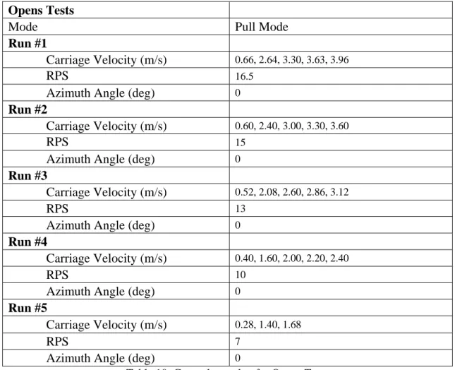
Opens Tests

Mode Pull Mode

Run #1

Carriage Velocity (m/s) 0.66, 2.64, 3.30, 3.63, 3.96

RPS 16.5

Run #2

RPS 15

Run #3

RPS 13

Run #4

RPS 10

Run #5

Carriage Velocity (m/s) 0.28, 1.40, 1.68

RPS 7

Table 10: General test plan for Opens Tests

5.4 Case 4 (a and b)

These tests were completed in the NRC-IOT Ice Tank in May of 2006 on a single podded propeller with a diameter of 200mm. For case 4a Pod B was static while for case 4b Pod A was static. The only test completed for this case was Opens Tests at low Froude numbers. This was mainly due to time constraints on the ice tank, and means that comparing the results with the other cases is difficult.

Opens Tests

Mode Pull Mode

Run #1

Carriage Velocity (m/s) 0, 0.13, 0.26, 0.39, 0.52, 0.65, 0.78, 0.91, 1.04

Pod 1

RPS 0

(21)

RPS 13

Run #2

Pod 1

RPS 13

Pod 2

RPS 0

Table 11: General test plan for Opens Tests

5.5 Case 5 (a and b)

Case 5a and 5b were also completed in the NRC-IOT Ice Tank in May of 2006. The tests were completed on two podded propellers operating simultaneously with a diameter of 200mm. Case 5a is the data collected for Pod A only while case 5b is the data collected for Pod B only. The following is a list of the types of experiments conducted: Air Friction and Bollard Runs, Opens Tests (0 deg azimuth), Oblique Flow Tests, and Dynamic Tests.

Mode Pull Mode

Run #1

Pod 1

RPS 0, 0.01, 0.1, 0.2, 0.5, 1, 2, 3, 4, 5, 6, 7, 8, 9, 10, 11, 12, 13, 14, 15

Pod 2

RPS 0

Run #2

Pod 1

RPS 0

Pod 2

RPS 0, 0.01, 0.1, 0.2, 0.5, 1, 2, 3, 4, 5, 6, 7, 8, 9, 10, _{11, 12, 13, 14, 15}

Run #4

Pod 1

(22)

Pod 2

RPS 0, 0.01, 0.1, 0.2, 0.5, 1, 2, 3, 4, 5, 6, 7, 8, 9, 10, _{11, 12, 13, 14, 15}

Table 12: General test plan for Air Friction Tests

Bollard Runs

Mode Pull Mode

Run #1

Pod 1

RPS 0, 0.01, 0.1, 0.2, 0.5, 1, 2, 3, 4, 5, 11, 12, 13

Pod 2

RPS 0

Run #2

Pod 1

RPS 0

Pod 2

RPS 0, 0.01, 0.1, 0.2, 0.5, 1, 2, 3, 4, 5, 11, 12, 13

Run #3

Pod 1

RPS 0, 0.01, 0.1, 0.2, 0.5, 1, 2, 3, 4, 5, 11, 12, 13

Pod 2

RPS 0, 0.01, 0.1, 0.2, 0.5, 1, 2, 3, 4, 5, 11, 12, 13

Table 13: General test plan for Bollards Tests

Opens Tests

Mode Pull Mode

Run #1 Carriage Velocity (m/s) 0, 0.13, 0.26, 0.39, 0.52, 0.65, 0.78, 0.91, 1.04, 1.17, 1.3, 1.56, 1.82, 2.08, 2.34, 2.47, 2.6, 2.86, 3.12 Pod 1

(23)

RPS 0, 0.1, 13

Pod 2

RPS 0, 0.1, 13

Table 14: General test plan for Open Tests

Mode Pull Mode

Run #1

Carriage Velocity (m/s) 0, 0.13, 0.26, 0.39, 0.52, 0.65, 0.78, 0.91, 1.04, 1.3, 1.56, 1.82, 2.08, 2.34, 2.47, 2.6, 2.86, 3.12

Pod 1

RPS 0, 0.1, 13

Pod 2

RPS 0, 0.1, 13

Run #2

Pod 1

RPS 0, 0.1, 13

Pod 2

RPS 0, 0.1, 13

Run #3

Pod 1

RPS 0, 0.1, 13

Pod 2

RPS 0, 0.1, 13

Run #4

Pod 1

RPS 0, 0.1, 13

(24)

Pod 2

RPS 0, 0.1, 13

Run #5

Pod 1

RPS 0, 0.1, 13

Pod 2

RPS 0, 0.1, 13

Dynamic Tests

Mode Pull Mode

Run#1 RPS 13 Carriage Velocity (m/s) 0, 0.13, 0.26, 0.39, 0.52, 0.65, 0.78, 0.91, 1.04, 1.17 Azimuth Rate 2, 5, 10, 20 Pod 1

Pod 2

Run #2

RPS 13

Carriage Velocity (m/s) 0, 0.13, 0.26, 0.39, 0.52, 0.65, 0.78, 0.91, 1.04, _1.17

Azimuth Rate 2, 5, 10, 20

Pod 1

Pod 2

Run #3 RPS 13 Carriage Velocity (m/s) 0, 0.13, 0.26, 0.39, 0.52, 0.65, 0.78, 0.91, 1.04, 1.17 Azimuth Rate 2, 5, 10, 20 Pod 1

(25)

Pod 2

Run #4 RPS 13 Carriage Velocity (m/s) 0, 0.13, 0.26, 0.39, 0.52, 0.65, 0.78, 0.91, 1.04, 1.17 Azimuth Rate 2, 5, 10, 20 Pod 1

Pod 2

Table 16: General test plan for Dynamic Tests

5.6 Case 6

This was another numerical simulation of the average pod geometry. They were computed for a single podded propeller with a 200mm diameter. Mohammed Islam and Dr. Pengfei Liu also completed the test using the program PROPELLA.

5.7 Case 7

Tests were conducted in May of 2006 in the NRC-IOT Ice Tank. The tests were conducted on a single podded propeller with a diameter of 200mm. The types of experiments

conducted were Air Friction and Bollard Runs, Opens Tests, and Oblique Flow Tests.

Mode Pull Mode

Run #1

RPS 0, 0.01, 0.1, 0.2, 0.5, 1, 2, 3, 4, 5, 11, 12, 13

Run #2

RPS 0, 0.01, 0.1, 0.2, 0.5, 1, 2, 3, 4, 5, 11, 12, 13

Run #3

RPS 0, 0.01, 0.1, 0.2, 0.5, 1, 2, 3, 4, 5, 11, 12, 13

(26)

Bollard Runs

Mode Pull Mode

Run #1

RPS 0, 0.01, 0.1, 0.2, 0.5, 1, 2, 3, 4, 5, 11, 12, 13

Run #2

RPS 0, 0.05, 0.1, 0.2, 0.3, 0.4, 0.5

Run #3

RPS 0, 0.01, 0.1, 0.2, 0.5, 1, 2, 3, 4, 5, 11, 12, 13

Run #4

RPS 0, 0.05, 0.1, 0.2, 0.3, 0.4, 0.5

Run #5

RPS 0, 0.01, 0.1, 0.2, 0.5, 1, 2, 3, 4, 5, 11, 12, 13

Run #6

RPS 0, 0.05, 0.1, 0.2, 0.3, 0.4, 0.5

Run #7

RPS 13

Run #8

RPS 13

Table 18: General test plan for Bollard Runs

Opens Tests

Mode Pull Mode

Run #1

Carriage Velocity (m/s) 1.30, 1.56, 1.82, 2.08, 2.34, 2.47, 2.60, 2.86, 3.12

RPS 13

(27)

Mode Pull Mode

Run #1

RPS 13

Run #2

RPS 13

6.0 DESCRIPTION OF EXPERIMENTS 6.1 Reynolds Number Effect Tests

Flow over full-scale propellers is fully turbulent at operating condition. Flow visualizations on propeller models have found that on model propellers with diameters between 168 and 355mm the boundary layer flow is mainly laminar on both the suction and pressure sides of the propeller blade at propeller Rn = nD2/ν below 1*106. Between Rn = 1*106 and 1*107

the boundary layer develops into fully developed turbulent flow, first on the suction side and then later on the pressure side. The exact or critical Rn at which the flow becomes fully

turbulent is dependent on factors such as the geometry, load conditions and flow conditions.6

Testing on model propellers must be at rotational speeds that allow the propeller to operate in a flow regime that minimizes laminar flow on the suction side or flow separation on the trailing edge. With respect to podded propulsion open water tests; this flow becomes particularly important in pulling pod configurations because the flow into the propeller is not affected by the turbulent wakes of the strut and pod.6

Through open water testing, researchers have found that the propeller performance becomes independent of the Rn at a level where the laminar flow is developing into

turbulent flow and this value can be found by completing Reynolds Number Effect Tests. The performance measurements are Thrust and Torque; the non-dimensional coefficients of Torque and Thrust are KQ and KT. If these values are plotted against Reynolds Numbers

there will be a point at which the Reynolds numbers does not affect the performance measurements. The performance parameters for both the large (D = 406mm) and small (D = 238mm) propellers stabilize at approximately 1-1.2 *106.

(28)

To perform a set of Reynolds effect tests a range of J values are chosen and then tested at a selection of rotation rates. The speed of advance is varied to give a selection of Reynolds Numbers. These Reynolds numbers are then plotted against performance parameters to see if the increase is having a significant effect on performance. The performance parameters are thrust and torque; the non-dimensional coefficients are KQ and KT. The equations for

both coefficients are shown above.

The following equation is used to determine Reynolds Number:

υ π 2 2 75 . 0 V (0.75 nD) c R_n = A +

Where: c0.75 = Chord length at 0.75 radius fraction of propeller = 0.095m

VA = Speed of advance

n = Shaft speed

D = Propeller diameter = 0.27m

ν = Kinematic viscosity = 1.139*10-6 m2/s

6.2 Air Friction Tests

Conducted by taking the pod(s) out of the water and running them in air. By completing these tests one can estimate the frictional losses in the system. This then allows the researcher to tare the torque values by subtracting this value from all the torque readings measured during the Opens Tests.

6.3 Bollard Runs

These are conducted when the carriage is at a stop. The propeller is run at operating speed (rps); which allows for the computation of Bollard Pull. The Bollard Pull for a propeller is the amount of thrust produced by the propeller when the vessel is stopped. This is

particularly important for vessels such as tugboats and icebreakers as they frequently operate at very low, next to zero, velocities.

6.4 Opens Tests (0 degree azimuth)

To illustrate the open water performance characteristics of the propeller a plot of KT, 10KQ,

η vs. J would be created, this is called the propeller performance chart. The equations to obtain these characteristics are described below in Table 5. For clarification, the definitions of all non-dimensional coefficients and terms shown in Table 5 are explained in further detail in Table 6. For completeness efficiency curves would be created and displayed for the data. These curves tend to be more sensitive to errors than thrust and torque coefficients, so therefore more emphasis is placed on observations in the thrust and torque coefficient data.

(29)

Performance Characteristic Data Reduction Equation

KTprop (Propeller Thrust Coefficient) /( )

4 2

D n T_prop ρ

KTunit (Unit Thrust Coefficient) /( )

4 2 D n T_unit ρ KQ (Torque Coefficient) /( ) 5 2 D n Q ρ J (Advance Coefficient) V/(nD)

ηprop (Propeller Efficiency (on Pod)) (KTpropJ)/(2πKQ)

ηunit (Unit Efficiency (on Pod)) (KTunitJ)/(2πKQ)

Where:

Tprop = Propeller Thrust n = Shaft Speed Tunit = Unit Thrust D = Propeller Diameter

Q = Torque V = Speed of Advance

ρ = Density

Table 21: Data Reduction Equations used in analysis Podded Propeller Test Definition

KTprop Non-dimensional form of the thrust of the propeller installed on the pod

KTunit Non-dimensional form of the unit thrust of the podded propeller

KQ Non-dimensional form of the torque on the propeller shaft

J Non-dimensional ratio of the advance speed to the shaft speed ηprop Open water efficiency of the propeller operating on the pod unit

ηunit Overall efficiency of the entire pod unit, which factors in the drag of the pod and strut

Tprop Axial component of force generated by the propeller when installed on the pod unit

Tunit Net axial thrust generated by the pod unit; includes the drag of the pod and its influence on the prop

Q The axial moment required to rotate the propeller at the desired shaft speed Table 22: Definitions of Data Reduction Terms

7.0 DESCRIPTION OF DATA ANALYSIS

For both the tests carried out in the NRC-IOT Ice Tank as well as the test case performed in the MUN Towing Tank ASCII data files were compiled for transfer to researchers personal computers when the trials were completed.

7.1 Interpreting the Raw Data (MUN Towing Tank Tests)

When the data is transferred it is ready to be post-processed. The interpretation was completed using Microsoft Excel 2000. A time series is plotted and averages are taken for each defined section of the run; these final averages are then used in the final analysis.

Figure 19 shows a typical run down the tank while performing an opens test. In the plot

below there are four sections; 1st. Nothing is on – both the carriage and propeller are still, 2nd. The carriage is turned on, but still doesn’t move forward, 3rd. The prop starts to move at a very low rps while the carriage remains stopped, 4th. The carriage is up to running speed

(30)

(approximately 2 m/s below) and the prop is running at desired rps. It should be noted that the plot below does not actually show rps, but shows the reading in volts. This would be changed to rps by multiplying by the appropriate constant.

After the averages are taken for each run the interpreted data can be transferred to a new Excel sheet where it is sorted according to run type (i.e. Third Quadrant Tests, Opens Tests, etc.) and advance coefficient, J. The physical quantities can then be non-dimensionalzed using the appropriate expression, as discussed in Section 7.4.

Figure 11: Typical plot of rps and Carriage Velocity for one run down the tank

7.2 Interpreting the Raw Data (NRC-IOT Ice Tank Tests)

Analysis of the tests was on going at the same time as the tests were running. A time series is plotted and averages are taken for each defined section of the run; these final averages are then used in the final analysis. Figure 24 shows a typical run down the tank while performing an opens test. In the plot below there are three defined sections; 1st. Nothing is on – both the carriage and propeller are still, 2nd. The propeller is up to desired rps (in this case approximately 15), 3rd. The carriage is up to running speed (below at about 3.1 m/s) and the prop is running at desired rps.

After the averages are taken for each run the interpreted data can be transferred to a Microsoft Excel sheet where it is sorted according to run type (i.e. Third Quadrant Tests,

(31)

Opens Tests, etc.) and advance coefficient, J (It’s customary to sort from J = 0 to J = 1.2). The physical quantities measured can then be non-dimensionalzed using the appropriate expressions, as discussed in Section 7.4.

Figure 12: Typical plot of rps and Carriage Velocity for one run down the tank

8.0 CALIBRATIONS

The method used to calibrate the global dynamometer as well as thrust and torque load cells was the linear least squares method. This method theorizes that if enough varied loads are applied in varied directions an accurate estimate of the calibration matrix can be obtained using an optimized linear least square fit. In other words, if the test apparatus can be loaded with enough independent loading cases to cover the expected use of the model during actual testing, then an accurate calibration matrix can be derived.

The algorithm used to obtain the linear least squares calibration matrix is: 1

)

]

][

([

]

][

[

]

[

C

=

L

a

T

a

T − (n,m) (m,z) (z,n) (n,z) (z,n)

Where: n is the number of balance components

m is the number of calibration coefficients per component, [m = n(n+3)/2] z is the number of loading cases

(32)

[L] defines the calculated distribution of the applied load P between the balance components for each loading case

[a] defines the actual distribution of the applied load P between the balance components for each loading case

8.1 Global Dynamometer

As stated above, the global dynamometer was calibrated using the linear least squares method. A total of forty-three cases were performed on the test set-up. This provided enough loading cases to provide an accurate calibration matrix.

z

x

y

Figure 13: Positive coordinate directions in 3-D space

From the above equation the following matrix of calibration coefficients can be obtained. The calibration coefficients can then be applied directly to the measured data to estimate the actual force reading. [L] and [a] matrices can be found in Appendix A.

[C] = 35.065 -0.62753 0.62753 -0.15249 0.08896 0.04254 4.702 61.447 -61.447 4.7079 -47.924 71.247 5.2784 24.211 -24.211 5.0931 -49.897 73.751 0.20125 0.97173 -0.97173 32.769 0.71655 1.5015 -0.00214 0.72505 -0.72505 -2.8303 36.846 1.6438 -0.17728 0.20692 -0.20692 -2.5681 0.75165 39.253

(33)

8.2 Thrust and Torque Load Cells

Calibrated in much the same way as the global dynamometer. Torque was produced by way of an adapter on the front of the pod where an arm could be attached (figure shown below). The results of the calibration are shown below in tables. [L] and [a] matrices for thrust and torque calibrations can be found in Appendix B.

Moment Arm

Figure 14: Photo showing how torque can be induced on the system

(34)

From the equation in Section 8.0 the following matrix of calibration coefficients can be obtained. The calibration coefficients can then be applied directly to the measured data to estimate the actual thrust and torque.

[C] = 65.9407 0.0064

0.0407 0.0115

9.0 RESULTS AND DISCUSSION

In the current study configurations of podded propellers were tested in either the NRC-IOT ice tank or the MUN Towing tank. The propellers were four bladed and in puller

configuration. There were also two cases where numerical methods were used to determine the performance characteristics of the podded propeller. The flowing is the results obtained from the Opens Tests along with comments on the experiments performed.

Kt_prop vs. J -0.3 -0.2 -0.1 0 0.1 0.2 0.3 0.4 0.5 0.6 0 0.2 0.4 0.6 0.8 1 1.2 1.4 J Case 1 Case 2 Case 3 Case 4a Case 5a Case 6 Case 7

(35)

Eff_prop vs. J -0.4 -0.2 0 0.2 0.4 0.6 0.8 1 0 0.2 0.4 0.6 0.8 1 1.2 1.4 J Case 1 Case 2 Case 3 Case 5a Case 5b Case 6 Case 7

Figure 17: Comparison of η_prop versus J

Kt_unit vs. J -0.2 -0.1 0 0.1 0.2 0.3 0.4 0.5 0 0.2 0.4 0.6 0.8 1 1.2 1.4 J Case 1 Case 2 Case 3 Case 4a Case 4b Case 5a Case 5b Case 6 Case 7

(36)

Eff_unit vs. J -0.4 -0.2 0 0.2 0.4 0.6 0.8 0 0.2 0.4 0.6 0.8 1 1.2 J Case 1 Case 2 Case 3 Case 5a Case 5b Case 6 Case 7 `

Figure 19: Comparison of η_unit versus J

Kt_pod vs. J -0.1 0 0.1 0.2 0.3 0.4 0.5 0.6 0 0.2 0.4 0.6 0.8 1 1.2 1.4 J Case 1 Case 6

(37)

Eff_pod vs. J 0 0.1 0.2 0.3 0.4 0.5 0.6 0.7 0.8 0.9 1 0 0.2 0.4 0.6 0.8 1 1.2 1.4 J Case 1 Case 6

Figure 21: Comparison of η_pod versus J

10Kq vs. J -0.1 0 0.1 0.2 0.3 0.4 0.5 0.6 0.7 0.8 0 0.2 0.4 0.6 0.8 1 1.2 1.4 J Case 1 Case 2 Case 3 Case 4a Case 4b Case 5a Case 5b Case 6 Case 7

(38)

From the above set of plots good comparison can be viewed for KT_unit, KT_pod, and 10KQ;

with fairly good results for KT_prop. KT_prop: all of the cases go negative between J = 1.05

and 1.15 approximately; KT_unit: all cases go negative between approximately J = 1.05 and

1.1; KT_pod: both cases go negative between J = 1.15 and 1.2; and 10KQ: the cases go

negative around approximately J = 1.2.

The efficiency curves show poorer quality results than the KT and 10KQ curves. This could

be possibly due to mechanical errors encountered during testing or a whole range of other possible sources. Whatever the cause may be it is not of great concern at this time, as the remainder of the opens tests show promising results; and as was stated earlier emphasis is placed on thrust and torque coefficients.

Unfortunately cases 4a and 4b were not completely finished and therefore it is difficult to compare the results to the rest of the cases. However, from the comparisons that can be made, it looks as though if the runs had been completed it is likely that the trend would have continued and the results would have been similar to the remainder of the results.

(39)

Kt_side vs. J -0.4 -0.3 -0.2 -0.1 0 0.1 0.2 0.3 0 0.2 0.4 0.6 0.8 1 1.2 1.4 J Case 1 Case 3 Case 5a Case 5b Case 6 Case 7

Figure 23: Comparison of KT_side versus J

Kt_vrt vs. J -0.04 -0.02 0 0.02 0.04 0.06 0.08 0.1 0.12 0.14 0.16 0 0.2 0.4 0.6 0.8 1 1.2 1 J .4 Case 1 Case 3 Case 5a Case 5b Case 6 Case 7

Figure 24: Comparison of KT_vrt versus J

The above two plots are the non-dimensional force coefficients obtained from the global dynamometer. The agreement between the cases isn’t very good; however there does seem to be a general trend in each of the plots.

(40)

10.0 RECOMMENDATIONS AND CONCLUSIONS

The following is a series of comments on the experiments performed and what steps should be taken in the future to confirm the results obtained.

Overall, the Opens Tests show good results. The tests correspond well with Principles of

Naval Architecture section on open water tests (page 145).5 However, since testing on podded propellers is still not as well know as conventional screw propellers, additional testing should be conducted to compare with this data analyzed. Further testing would provide researchers with valuable knowledge about podded propellers as well as providing a solid base to compare future tests.

Further Reynolds effect tests should be conducted on podded propellers to verify if testing on podded propellers can be completed at lower Reynolds Numbers than recommended by ITTC (i.e. less than 1*106).

Testing thus far by NRC has provided the institute with priceless information and knowledge about the performance characteristics of podded propulsors. Further testing would compliment the testing executed so far and would help to further expand the

researcher’s knowledge. Plans now being made include the building of a model icebreaker hull to which two podded propellers will be fitted and self-propulsion tests will be

conducted.

11.0 ACKNOWLEDGMENTS

I would like to express their gratitude to the National Research Council (NRC) and Memorial University of Newfoundland (MUN) for their financial and other support. Thanks are also extended to the staff in both the Ice tank at Institute for Ocean Technology (IOT) and the staff in the MUN Towing tank, without whose assistance the tests would not have been completed. I would also like to thank Dr. Ayhan Akinturk, whose support and guidance throughout my work term has allowed me to expand my engineering knowledge.

12.0 REFERENCES

1) Islam, M., Veitch, B., Bose, N., Liu, P., (2006). “Hydrodynamic Characteristics of Puller Podded Propulsors with Tapered Hub Propellers.”

2) National Research Council – Institute for Ocean Technology website.

URL: http://iot-ito.nrc-cnrc.gc.ca/facilities/it_e.html

3) Oceanic Consulting Corporation Website>Facilities>58m Towing Tank. URL: http://www.oceaniccorp.com/FacilityDetails.asp?id=2

4) Bell, J., (2005). “TDC Podded Propeller Drive.” Institute for Ocean Technology, NRC: Report No. LM – 2005 – 01

5) MacNeill, A., Taylor, R., Malloy, S., Bose, N., Veitch, B., Randell, T., Liu, P., (2004). “Design of Model Pod Test Unit.” Proceedings of the 1st International

(41)

Conference on Technological Advances in Podded Propulsion. Newcastle University, UK, April.

6) Jessup, S., Bose, N., Dugué, C., Esposito, P.G., Holtrop, J., Lee, J.T., Mewis, F., Pustoshny, A., Salvatore, F., Shirose, Y., (2003). Proceedings of the 23rd ITTC - Volume 1: The Propulsion Committee, ITTC 23 USA

7) Taylor, R., (2005). “Experimental Investigation of the Influence of Hub Taper Angle on the Performance of Push and Pull Configuration Podded Propellers.” Masters of Engineering Thesis, Memorial University of Newfoundland, Canada. 8) Lewis, E., “Principles of Naval Architecture. Volume 2: Resistance, Propulsion and

(42)

(43)

A-1: Matrix of coefficients obtained from measured data ([a] matrix)

a1 1 0.000195 a1 2 -0.000002 a1 3 -0.000324 a1 4 -0.014440 a1 5 0.009645 a1 6 0.031223 a2 1 0.000203 a2 2 -0.000092 a2 3 -0.000196 a2 4 -0.018068 a2 5 0.022992 a2 6 0.021882 a3 1 0.000217 a3 2 -0.000170 a3 3 -0.000059 a3 4 -0.014240 a3 5 0.032529 a3 6 0.009249 a4 1 0.000216 a4 2 -0.000239 a4 3 0.000063 a4 4 -0.004432 a4 5 0.036409 a4 6 -0.003590 a5 1 0.020020 a5 2 0.000525 a5 3 -0.000728 a5 4 0.018484 a5 5 0.005772 a5 6 -0.003839 a6 1 0.019963 a6 2 -0.006626 a6 3 0.006172 a6 4 0.015276 a6 5 0.013996 a6 6 -0.008683 a7 1 0.019914 a7 2 -0.012950 a7 3 0.012284 a7 4 0.015068 a7 5 0.021208 a7 6 -0.015380 a8 1 0.019877 a8 2 -0.016941 a8 3 0.016174 a8 4 0.020498 a8 5 0.025721 a8 6 -0.024769 a9 1 0.028344 a9 2 -0.000764 a9 3 0.000544 a9 4 0.034327 a9 5 -0.000415 a9 6 -0.032013 a10 1 0.028194 a10 2 -0.014058 a10 3 0.013405 a10 4 0.034140 a10 5 -0.000459 a10 6 -0.031759 a11 1 0.028117 a11 2 -0.024495 a11 3 0.023504 a11 4 0.032846 a11 5 -0.000490 a11 6 -0.030490 a12 1 0.028090 a12 2 -0.027440 a12 3 0.026370 a12 4 0.033828 a12 5 -0.000502 a12 6 -0.031385 a13 1 -0.019738 a13 2 -0.000275 a13 3 -0.000008 a13 4 -0.038168 a13 5 0.005998 a13 6 0.049189 a14 1 -0.019698 a14 2 0.010259 a14 3 -0.010146 a14 4 -0.040563 a14 5 0.018221 a14 6 0.039655 a15 1 -0.019731 a15 2 0.015956 a15 3 -0.015600 a15 4 -0.035808 a15 5 0.024800 a15 6 0.028816 a16 1 -0.019746 a16 2 0.016634 a16 3 -0.016238 a16 4 -0.026980 a16 5 0.025666 a16 6 0.019722 a17 1 -0.028211 a17 2 -0.000968 a17 3 0.000681 a17 4 -0.034967 a17 5 -0.000371 a17 6 0.032725 a18 1 -0.028311 a18 2 -0.014139 a18 3 0.013359 a18 4 -0.034467 a18 5 -0.000213 a18 6 0.032102 a19 1 -0.028385 a19 2 -0.024052 a19 3 0.022892 a19 4 -0.034383 a19 5 -0.000095 a19 6 0.031908 a20 1 -0.028418 a20 2 -0.027663 a20 3 0.026368 a20 4 -0.034127 a20 5 -0.000048 a20 6 0.031622 a21 1 0.000057 a21 2 -0.000042 a21 3 -0.000181 a21 4 0.023576 a21 5 -0.018298 a21 6 0.022486 a22 1 0.000329 a22 2 0.000155 a22 3 -0.000452 a22 4 -0.023445 a22 5 0.008822 a22 6 0.040493 a23 1 0.000261 a23 2 -0.000034 a23 3 -0.000258 a23 4 -0.029015 a23 5 0.028406 a23 6 0.026982 a24 1 0.000213 a24 2 -0.000215 a24 3 -0.000053 a24 4 -0.023606 a24 5 0.041982 a24 6 0.008951 a25 1 0.000139 a25 2 -0.000339 a25 3 0.000111 a25 4 -0.009037 a25 5 0.047180 a25 6 -0.009609 a26 1 0.000015 a26 2 -0.000066 a26 3 -0.000159 a26 4 0.029226 a26 5 -0.029007 a26 6 0.027356 a27 1 0.020077 a27 2 -0.000223 a27 3 -0.000021 a27 4 0.011221 a27 5 0.006718 a27 6 0.001966 a28 1 0.019971 a28 2 -0.010421 a28 3 0.009842 a28 4 0.007381 a28 5 0.018352 a28 6 -0.005547 a29 1 0.019851 a29 2 -0.018892 a29 3 0.018062 a29 4 0.009533 a29 5 0.027997 a29 6 -0.016769 a30 1 0.019215 a30 2 -0.023189 a30 3 0.022280 a30 4 0.018896 a30 5 0.033847 a30 6 -0.030591 a31 1 0.028280 a31 2 0.000682 a31 3 -0.000855 a31 4 0.033118 a31 5 -0.000177 a31 6 -0.030320 a32 1 0.028144 a32 2 -0.017098 a32 3 0.016404 a32 4 0.032827 a32 5 0.000180 a32 6 -0.030297

(44)

a33 1 0.028026 a33 2 -0.030886 a33 3 0.029790 a33 4 0.032006 a33 5 0.000456 a33 6 -0.029720 a34 1 0.028040 a34 2 -0.029491 a34 3 0.028441 a34 4 0.032729 a34 5 0.000435 a34 6 -0.030377 a35 1 0.028527 a35 2 0.029442 a35 3 -0.028780 a35 4 0.034110 a35 5 -0.000845 a35 6 -0.030813 a36 1 -0.020171 a36 2 0.000493 a36 3 -0.000663 a36 4 0.007872 a36 5 0.007335 a36 6 0.004525 a37 1 -0.020194 a37 2 -0.012607 a37 3 0.011942 a37 4 0.012466 a37 5 -0.007498 a37 6 0.014456 a38 1 -0.019379 a38 2 0.018198 a38 3 -0.017706 a38 4 -0.037984 a38 5 0.027990 a38 6 0.028190 a39 1 -0.019522 a39 2 0.020608 a39 3 -0.020022 a39 4 -0.028954 a39 5 0.030784 a39 6 0.016922 a40 1 -0.028262 a40 2 -0.001292 a40 3 0.001015 a40 4 -0.033571 a40 5 -0.000138 a40 6 0.031957 a41 1 -0.028133 a41 2 0.015615 a41 3 -0.015197 a41 4 -0.034279 a41 5 0.000035 a41 6 0.032476 a42 1 -0.028425 a42 2 -0.026347 a42 3 0.025061 a42 4 -0.033592 a42 5 -0.000433 a42 6 0.032207 a43 1 -0.028444 a43 2 -0.029187 a43 3 0.027782 a43 4 -0.034047 a43 5 -0.000482 a43 6 0.032664

(45)

A-2: Matrix of coefficients obtained from calculated data ([L] matrix)

f1 1 0.000000 f1 2 0.000000 f1 3 0.000000 f1 4 -0.532872 f1 5 0.352286 f1 6 1.180636 f2 1 0.000000 f2 2 0.000000 f2 3 0.000000 f2 4 -0.657899 f2 5 0.831907 f2 6 0.826042 f3 1 0.000000 f3 2 0.000000 f3 3 0.000000 f3 4 -0.519859 f3 5 1.183014 f3 6 0.336895 f4 1 0.000000 f4 2 0.000000 f4 3 0.000000 f4 4 -0.155739 f4 5 1.311528 f4 6 -0.155739 f5 1 0.707135 f5 2 0.000000 f5 3 0.000000 f5 4 0.467414 f5 5 0.249101 f5 6 -0.009380 f6 1 0.707135 f6 2 -0.301072 f6 3 0.301072 f6 4 0.379007 f6 5 0.588241 f6 6 -0.260113 f7 1 0.707135 f7 2 -0.521473 f7 3 0.521473 f7 4 0.476615 f7 5 0.836509 f7 6 -0.605989 f8 1 0.707135 f8 2 -0.602145 f8 3 0.602145 f8 4 0.734085 f8 5 0.927381 f8 6 -0.954331 f9 1 1.000050 f9 2 0.000000 f9 3 0.000000 f9 4 1.193901 f9 5 0.000000 f9 6 -1.193901 f10 1 1.000050 f10 2 -0.425785 f10 3 0.425785 f10 4 1.193901 f10 5 0.000000 f10 6 -1.193901 f11 1 1.000050 f11 2 -0.737481 f11 3 0.737481 f11 4 1.193901 f11 5 0.000000 f11 6 -1.193901 f12 1 1.000050 f12 2 -0.851093 f12 3 0.851093 f12 4 1.193901 f12 5 0.000000 f12 6 -1.193901 f13 1 -0.707135 f13 2 0.000000 f13 3 0.000000 f13 4 -1.221001 f13 5 0.249101 f13 6 1.679035 f14 1 -0.707135 f14 2 0.301072 f14 3 -0.301072 f14 4 -1.309408 f14 5 0.588241 f14 6 1.428302 f15 1 -0.707135 f15 2 0.521473 f15 3 -0.521473 f15 4 -1.211800 f15 5 0.836509 f15 6 1.082426 f16 1 -0.707135 f16 2 0.602145 f16 3 -0.602145 f16 4 -0.954331 f16 5 0.927381 f16 6 0.734085 f17 1 -1.000050 f17 2 0.000000 f17 3 0.000000 f17 4 -1.193901 f17 5 0.000000 f17 6 1.193901 f18 1 -1.000050 f18 2 -0.425785 f18 3 0.425785 f18 4 -1.193901 f18 5 0.000000 f18 6 1.193901 f19 1 -1.000050 f19 2 -0.737481 f19 3 0.737481 f19 4 -1.193901 f19 5 0.000000 f19 6 1.193901 f20 1 -1.000050 f20 2 -0.851570 f20 3 0.851570 f20 4 -1.193901 f20 5 0.000000 f20 6 1.193901 f21 1 0.000000 f21 2 0.000000 f21 3 0.000000 f21 4 0.803503 f21 5 -0.606956 f21 6 0.803503 f22 1 0.000000 f22 2 0.000000 f22 3 0.000000 f22 4 -0.895679 f22 5 0.352286 f22 6 1.543442 f23 1 0.000000 f23 2 0.000000 f23 3 0.000000 f23 4 -1.073651 f23 5 1.035011 f23 6 1.038690 f24 1 0.000000 f24 2 0.000000 f24 3 0.000000 f24 4 -0.877155 f24 5 1.534800 f24 6 0.342405 f25 1 0.000000 f25 2 0.000000 f25 3 0.000000 f25 4 -0.358843 f25 5 1.717735 f25 6 -0.358843 f26 1 0.000000 f26 2 0.000000 f26 3 0.000000 f26 4 1.006606 f26 5 -1.013163 f26 6 1.006606 f27 1 0.707135 f27 2 0.000000 f27 3 0.000000 f27 4 0.268720 f27 5 0.249101 f27 6 0.189314 f28 1 0.707135 f28 2 -0.428567 f28 3 0.428567 f28 4 0.085029 f28 5 0.731856 f28 6 -0.109750 f29 1 0.707135 f29 2 -0.742299 f29 3 0.742299 f29 4 0.223971 f29 5 1.085257 f29 6 -0.602093 f30 1 0.707135 f30 2 -0.857133 f30 3 0.857133 f30 4 0.590470 f30 5 1.214610 f30 6 -1.097945 f31 1 1.000050 f31 2 0.000000 f31 3 0.000000 f31 4 1.193901 f31 5 0.000000 f31 6 -1.193901 f32 1 1.000050 f32 2 -0.606091 f32 3 0.606091 f32 4 1.193901 f32 5 0.000000 f32 6 -1.193901

(46)

f33 1 1.000050 f33 2 -1.128514 f33 3 1.128514 f33 4 1.193901 f33 5 0.000000 f33 6 -1.193901 f34 1 1.000050 f34 2 -1.115207 f34 3 1.115207 f34 4 1.193901 f34 5 0.000000 f34 6 -1.193901 f35 1 1.000050 f35 2 1.115207 f35 3 -1.115207 f35 4 1.193901 f35 5 0.000000 f35 6 -1.193901 f36 1 -0.707135 f36 2 0.000000 f36 3 0.000000 f36 4 0.210873 f36 5 0.249101 f36 6 0.247160 f37 1 -0.707135 f37 2 -0.428567 f37 3 0.428567 f37 4 0.373005 f37 5 -0.233653 f37 6 0.567784 f38 1 -0.707135 f38 2 0.682915 f38 3 -0.682915 f38 4 -1.396504 f38 5 1.018365 f38 6 1.085275 f39 1 -0.707135 f39 2 0.857133 f39 3 -0.857133 f39 4 -1.097945 f39 5 1.214610 f39 6 0.590470 f40 1 -1.000050 f40 2 0.000000 f40 3 0.000000 f40 4 -1.193901 f40 5 0.000000 f40 6 1.193901 f41 1 -1.000050 f41 2 0.606091 f41 3 -0.606091 f41 4 -1.193901 f41 5 0.000000 f41 6 1.193901 f42 1 -1.000050 f42 2 -1.049780 f42 3 1.049780 f42 4 -1.193901 f42 5 0.000000 f42 6 1.193901 f43 1 -1.000050 f43 2 -1.212181 f43 3 1.212181 f43 4 -1.193901 f43 5 0.000000 f43 6 1.193901

(47)

(48)

(49)

B-1: Matrix of coefficients obtained from measured data

a1 1 0.008517 a1 2 4.799733 a2 1 -0.010700 a2 2 -4.780244 a3 1 -0.000339 a3 2 6.713952 a4 1 -0.000337 a4 2 -6.676090 a5 1 0.014632 a5 2 0.001815 a6 1 -0.015982 a6 2 -0.000193 a7 1 -0.016897 a7 2 -0.002923 a8 1 0.014210 a8 2 -0.003161 Matrix of coefficients obtained from measured data

(50)

B-2: Matrix of coefficients obtained from calculated data

f1 1 0.707100 f1 2 0.053881 f2 1 -0.707100 f2 2 -0.053881 f3 1 0.000000 f3 2 0.076200 f4 1 0.000000 f4 2 -0.076200 f5 1 1.000000 f5 2 0.000000 f6 1 -1.000000 f6 2 0.000000 f7 1 -1.000000 f7 2 0.000000 f8 1 1.000000 f8 2 0.000000 Matrix of coefficients obtained from calculated data

(51)

(52)

APPENDIX C: Data Acquisition System Channel Set-up for

NRC-IOT Tests

(53)

DAS PLAN

Project Name: T.C. Azipod Project Number: 42_2085_16

Signal Conditioner: Custom IOTech Date: 9-Dec-05

Sampling Rate: 5Khz Generated by: James E. Williams

GDAC CHAN # IOTech# DESCRIPTION/DEVICE SERIAL # BAR-CODE RANGE FILTER EXC. Volts Gain Offset Cal. Factor

1 0 Ch00-0-0 Pod 1, Fxa, Port E50407 200203 250 lbf 1Khz 10 150

2 1 Ch00-0-1 Pod 1, Fy1a E50185 200201 250 lbf 1Khz 10 150

3 2 Ch00-0-2 Pod 1, Fy2a E50406 200207 250 lbf 1Khz 10 150

4 3 Ch00-0-3 Pod 1, Fz1a E50400 200204 250 lbf 1Khz 10 150

5 4 Ch00-0-4 Pod 1, Fz2a E50204 200205 250 lbf 1Khz 10 150

6 5 Ch00-0-5 Pod 1, FZ3a E50184 200208 250 lbf 1Khz 10 150

7 6 Ch00-0-6 spare 1Khz 5

8 7 Ch00-0-7 spare 1Khz 5

9 8 Ch00-1-0 Pod 2, Fxb, Starboard E50413 200206 250 lbf 1Khz 10 150

10 9 Ch00-1-1 Pod 2, Fy1b E50384 200198 250 lbf 1Khz 10 150

11 10 Ch00-1-2 Pod 2, Fy2b E50170 200199 250 lbf 1Khz 10 150

12 11 Ch00-1-3 Pod 2, Fz1b E50417 200200 250 lbf 1Khz 10 150

13 12 Ch00-1-4 Pod 2, Fz2b E50403 200197 250 lbf 1Khz 10 150

14 13 Ch00-1-5 Pod 2, FZ3b E50194 200202 250 lbf 1Khz 10 150

15 14 Ch00-1-6 spare 1Khz 5

16 15 Ch00-1-7 spare 1Khz 5

17 16 Ch01-0-0 Pod 1, Thrust, Ta 21316 50 lbf 1Khz N/A 4.4

18 17 Ch01-0-1 Pod 1, Torque, Qa A 1Khz N/A 5.39

(54)

20 19 Ch01-0-3 1Khz N/A

21 20 Ch01-1-0 Pod 2 Thrust ,Tb 21320 50 lbf 1Khz N/A 3.45

22 21 Ch01-1-1 Pod 2, Torque,Qb B 1Khz N/A 5.39

23 22 Ch01-1-2 Pod 2 RPS 1Khz N/A ?

24 23 Ch01-1-3 DAS Sync signal 1Khz N/A

25 RS232 Ch1 Pod 1 Azimithing angle 360 degs na

26 RS232 Ch2 Pod 2 Azumithing angle 360 degs na

27 RS232 Ch3 Pod 1 Blade Angle

28 RS232 Ch4 Pod 2 Blade Angle

29 RS232 Ch5 Pod 1 RPS

30 RS232 Ch6 Pod 2 RPS

30 RS232 Ch7 DAS Sync signal

Industrial pc: Telem # : PC004026 IP # Barcode:

(55)

(56)

(57)

D-1: Reynolds Number Effect Tests

Bollard -10 -5 0 5 10 15 20 -12 -7 -2 3 8 rps Kt_pod Kt_prop Kt_unit 10Kq Bollard -0.001 -0.0005 0 0.0005 0.001 0.0015 0.002 0.0025 0.003 0.0035 0.004 -12 -7 -2 3 8 rps Eff_pod Eff_prop Eff_unit

(58)

Bollard -1000 -500 0 500 1000 1500 -15 -10 -5 0 5 10 15 rps Kt_side Kt_vrt

(59)

D-2: Opens Tests Results

Opens Tests -0.1 0 0.1 0.2 0.3 0.4 0.5 0.6 0.7 0.8 0 0.2 0.4 0.6 0.8 1 1.2 J Kt_pod Kt_prop Kt_unit 10Kq Opens Tests -0.6 -0.4 -0.2 0 0.2 0.4 0.6 0.8 1 0 0.2 0.4 0.6 0.8 1 1.2 J Eff_pod Eff_prop Eff_unit

(60)

Opens Tests 0 0.005 0.01 0.015 0.02 0.025 0.03 0.035 0.04 0.045 0.05 0 0.2 0.4 0.6 0.8 1 1.2 J Kt_side Kt_vrt

(61)

D-3: Third Quadrant Runs

Third Quadrant Run

-0.1 0 0.1 0.2 0.3 0.4 0.5 0.6 0.7 0 0.1 0.2 0.3 0.4 0.5 0.6 J Kt_pod Kt_prop Kt_unit 10Kq

Third Quadrant Run

-0.1 0 0.1 0.2 0.3 0.4 0.5 0 0.1 0.2 0.3 0.4 0.5 0.6 J Eff_pod Eff_prop Eff_unit

(62)

Third Quadrant Run -0.02 -0.01 0 0.01 0.02 0.03 0.04 0 0.1 0.2 0.3 0.4 0.5 0.6 J Kt_side Kt_vrt

(63)

D-4: Oblique Flow Tests

9 Degrees Azimuth Angle

-0.2 -0.1 0 0.1 0.2 0.3 0.4 0.5 0.6 0.7 0 0.2 0.4 0.6 0.8 1 1.2 1.4 J Kt_pod Kt_prop Kt_unit 10Kq

9 Degrees Azimuth Angle

-1 -0.8 -0.6 -0.4 -0.2 0 0.2 0.4 0.6 0.8 1 0 0.2 0.4 0.6 0.8 1 1.2 J Eff_pod Eff_prop Eff_unit

(64)

9 Degrees Azimuth Angle -0.15 -0.1 -0.05 0 0.05 0.1 0 0.2 0.4 0.6 0.8 1 1.2 1.4 J Kt_side Kt_vrt

9 Degrees Azimuth Angle - Quadrant Three

-0.3 -0.2 -0.1 0 0.1 0.2 0.3 0.4 0.5 0 0.1 0.2 0.3 0.4 0.5 0.6 0.7 J Kt_pod Kt_prop Kt_unit 10Kq

(65)

9 Degrees Azimuth Angle - Quadrant Three 0 0.1 0.2 0.3 0.4 0.5 0.6 0 0.1 0.2 0.3 0.4 0.5 0.6 0.7 J Eff_pod Eff_prop Eff_unit

9 Degrees Azimuth Angle - Quadrant Three

-0.02 -0.01 0 0.01 0.02 0.03 0.04 0.05 0.06 0 0.1 0.2 0.3 0.4 0.5 0.6 0.7 J Kt_side Kt_vrt

(66)

-9 Degrees Azimuth Angle -0.2 -0.1 0 0.1 0.2 0.3 0.4 0.5 0.6 0.7 0.8 0 0.2 0.4 0.6 0.8 1 1.2 1.4 J Kt_pod Kt_prop Kt_unit 10Kq

-9 Degrees Azimuth Angle

-0.6 -0.4 -0.2 0 0.2 0.4 0.6 0.8 1 0 0.2 0.4 0.6 0.8 1 1.2 J Eff_pod Eff_prop Eff_unit

(67)

-9 Degrees Azimuth Angle 0 0.01 0.02 0.03 0.04 0.05 0.06 0.07 0.08 0.09 0.1 0 0.2 0.4 0.6 0.8 1 1.2 1.4 J Kt_side Kt_vrt

-9 Degrees Azimuth Angle - Quadrant Three

-0.2 -0.1 0 0.1 0.2 0.3 0.4 0.5 0.6 0 0.1 0.2 0.3 0.4 0.5 0.6 0.7 J Kt_pod Kt_prop Kt_unit 10Kq

(68)

-9 Degrees Azimuth Angle - Quadrant Three -0.2 -0.1 0 0.1 0.2 0.3 0.4 0.5 0.6 0 0.1 0.2 0.3 0.4 0.5 0.6 0.7 J Eff_pod Eff_prop Eff_unit

-9 Degrees Azimuth Angle - Quadrant Three

-0.05 -0.04 -0.03 -0.02 -0.01 0 0.01 0 0.1 0.2 0.3 0.4 0.5 0.6 0.7 J Kt_side Kt_vrt

(69)

(70)

(71)

E-1: Reynolds Number Effect Tests

-0.1 0 0.1 0.2 0.3 0.4 0.5 0.6 0 100000 200000 300000 400000 500000 600000 700000 Rn K t -0.2 -0.1 0 0.1 0.2 0.3 0.4 0.5 0 100000 200000 300000 400000 500000 600000 700000 Rn Kt _ u n i

(72)

-0.1 0 0.1 0.2 0.3 0.4 0.5 0.6 0.7 0.8 0 100000 200000 300000 400000 500000 600000 700000 Rn K q -0.3 -0.25 -0.2 -0.15 -0.1 -0.05 0 0.05 0.1 0.15 0.2 0.25 0 100000 200000 300000 400000 500000 600000 700000 Rn K t_u n it _sid e_f o r

(73)

E-2: Air Friction Tests

Thrust, N -15 -10 -5 0 5 10 15 0 2 4 6 8 10 12 14 16 rps P rop . Th ru s t, Torque, Nm -0.01 -0.005 0 0.005 0.01 0.015 0.02 0.025 0.03 0.035 0 2 4 6 8 10 12 14 16 rps P rop . To rq ue , N

(74)

Glo_Fxb, N -0.35 -0.3 -0.25 -0.2 -0.15 -0.1 -0.05 0 0.05 0.1 0 2 4 6 8 10 12 14 rps U n it T h ru s t, 16 Glo_Fyb, N -1.5 -1 -0.5 0 0.5 1 1.5 2 0 2 4 6 8 10 12 14 rps Un it S id e F o rc 16 e

(75)

E-3: Bollard Runs

Thrust, N -100 -50 0 50 100 150 200 250 -2 0 2 4 6 8 10 12 14 16 rps P rop. T h ru s t, Torque, Nm -1 0 1 2 3 4 5 6 -2 0 2 4 6 8 10 12 14 16 rps P rop. T o rque, N

(76)

Glo_Fxb, N -20 0 20 40 60 80 100 120 140 160 180 -2 0 2 4 6 8 10 12 14 rps Un it T h ru s t 16 , Glo_Fyb, N -80 -60 -40 -20 0 20 40 60 80 100 120 -2 0 2 4 6 8 10 12 14 rps U n it S ide F o rc 16 e