Numerical study of the linear polarization resistance technique applied to reinforced concrete for corrosion assessment

HAL Id: hal-00692545

https://hal.archives-ouvertes.fr/hal-00692545

Submitted on 30 Apr 2012

HAL is a multi-disciplinary open access

archive for the deposit and dissemination of

sci-entific research documents, whether they are

pub-lished or not. The documents may come from

teaching and research institutions in France or

abroad, or from public or private research centers.

L’archive ouverte pluridisciplinaire HAL, est

destinée au dépôt et à la diffusion de documents

scientifiques de niveau recherche, publiés ou non,

émanant des établissements d’enseignement et de

recherche français ou étrangers, des laboratoires

publics ou privés.

Numerical study of the linear polarization resistance

technique applied to reinforced concrete for corrosion

assessment

Antoine Clément, S. Laurens, Ginette Arliguie, D. Deby

To cite this version:

Antoine Clément, S. Laurens, Ginette Arliguie, D. Deby. Numerical study of the linear polarization

resistance technique applied to reinforced concrete for corrosion assessment. European Journal of

Environmental and Civil Engineering, Taylor & Francis, 2012, pp.17. �10.1080/19648189.2012.668012�.

�hal-00692545�

Submitted to European Journal Of Environmental and Civil Engineering, 2012

Numerical study of the linear polarization

resistance technique applied to reinforced

concrete for corrosion assessment

A. Clément – S. Laurens – G. Arliguie – F. Deby

Université de Toulouse ; UPS, INSA ; LMDC (Laboratoire Matériaux et Durabilité des Constructions)

135, Avenue de Rangueil F-31077 Toulouse Cedex 4 ; France Stephane.laurens@insa-toulouse.fr

RÉSUMÉ. La technique de résistance de polarisation linéaire (Rp) est utiisée de plus en plus

fréquemment pour évaluer la cinétique de corrosion des aciers dans le béton armé. Cependant, la technique souffre d’un manque de fiabilité. Afin de mieux appréhender la physique de la mesure, des simulations numériques ont été réalisées. Plusieurs dispositifs ont été simulés. Ces expériences numériques ont permis d’éprouver la robustesse du protocole RILEM dédié à la mesure de Rp in situ. Les résultats montrent que les mesures réalisées au

moyen de sondes annulaires constituent un problème physique tridimensionnel qui doit être mieux pris en compte par le protocole RILEM. En particulier, la distribution non uniforme du courant polarisant constitue une source d’erreur importante dans la mesure où elle n’est pas considérée dans la recommandation RILEM. Enfin, les simulations ont révélé une forme de complexité supplémentaire induite par l’utilisation d’anneaux de garde pour le confinement du courant polarisant.

ABSTRACT. The linear polarization resistance (LPR) technique is increasingly being

implemented to assess the corrosion rate of steel reinforcements in concrete. However, a lack of reliability is often observed experimentally. In order to improve the physical comprehension of the LPR technique, FEM simulations were performed. Several measurement devices using annular and rectangular probe geometries were simulated and the numerical experimentation allowed the relevance of RILEM recommendations for on-site measurements to be tested. It was shown that the LPR measurement using annular counter-electrodes with confining devices was a real three-dimensional physical problem and the non-uniform distribution of the polarizing current on the steel surface is actually a major source of error since it is not taken into account by the usual protocols. Moreover, it was found that some complexity was induced by the use of guard-rings.

MOTS-CLÉS: Corrosion, béton armé, résistance de polarisation linéaire, mesures in situ, simulation numérique

KEYWORDS: Corrosion, steel reinforced concrete, linear polarization resistance, on-site

1. Introduction

Corrosion is the main source of damage in reinforced concrete structures. Therefore, it is crucial for service life prediction to be able to assess the corrosion rate of steel. The Linear Polarization Resistance (LPR) technique theoretically provides the corrosion current density, and thus the corrosion rate of steel, by measuring the polarization resistance (Rp). According to several assumptions, the

corrosion current density jcorr [A.m-2] and the polarization resistance Rp [.m2] are

linked by the Stern-Geary relation (Stern et al., 1957): p

corr R

B

j  _[1]

Where B [V] is a factor defined below, which depends on anodic and cathodic Tafel slopes.

Although the LPR technique is now widely used, a large dispersion is observed in Rp determination. The French research project „Benchmark des poutres de la

Rance‟ used common commercial devices and laboratory devices to assess the corrosion rate of corroded beams (Poupard et al., 2005). Results showed differences of a factor often higher than 20 between the devices tested. This lack of reliability may be explained in various ways. First, the technique is often implemented beyond the theoretical limits. It should be used only in cases of uniform corrosion induced, for example, by concrete carbonation (Stern et al., 1957) (Gulikers, 2005) (Song, 2000). Moreover, the polarization should be limited (lower than 20 mV / Ecorr) in order to remain in the linear polarization range (RILEM, 2004) (Nygaard et al., 2009). The second main issue is that the Rp calculation usually assumes uniform

current density distribution on a specific surface of the corroding rebar, and consequently uniform polarization. Actually, according to the physical geometry, there is no reason for current density distribution and polarization to be uniform. Furthermore, current distribution is highly influenced by environmental and geometrical factors.

The modeling of corrosion propagation in reinforced concrete has been a field of intensive research, so scientific literature can be found easily. The main theoretical considerations are reviewed in (Warkus et al., 2006a) (Raupach, 2006) and a sample of applications is given in (Gulikers et al., 2006) (Warkus et al., 2006) (Nasser et al., 2010). Comparatively, there has been little work published specifically on LPR simulations. Resistance networks are often implemented to simulate the measurement. Wojtas used a 2D network to study the ability of a guard-ring to confine the current along the rebar axis, and showed that it was not possible to obtain a reliable Rp value for the full range of corrosion current (Wojtas, 2004). In (Feliu et al., 1995), the current distribution is considered in the rebar cross-sectional plane. It proves not to be uniform and, in cases of active corrosion, can lead to an overestimation of current corrosion by between 10% and 30% depending on the geometry. Kranc and Sagües considered radial symmetry of the problem and simulated the measurement according to a transient method (Kranc et al., 1993).

They studied the effect of guard ring and counter-electrode size with respect to cover depth and the accuracy of the results for local or uniform corrosion. The study indicated that the measurement was successful only in cases of uniform corrosion with an electrode size larger than the cover depth. In order to take account of the effect on polarized length of some parameters influencing the measurement (such as concrete resistivity), Tang and Fu used a 2D FEM model of a new linear device and developed a specific formula to interpret the measurement (Tang et al., 2006). The combination of this new device with the formula gives results comparable to other commercial devices but much faster. A more complete study is reported in (Janusz, 1993) with a 2D and 3D FEM model in the steady state. Several parameters, such as corrosion intensity, probe dimensions, cover depth and concrete resistivity, were investigated by focusing on potential and current mapping. However, no major measurement improvements were proposed from the numerous simulations carried out.

Despite the simulation works presented above, some questions remain as to the quantitative effects of the factors that most influence LPR measurements. In this field, the research presented below aimed to perform FEM experiments to analyze the effects of probe geometry on the polarizing current distribution for a complete 3D model, and to quantify errors on Rp and jcorr measurements.

2. Theoretical background

2.1. Corrosion

Corrosion of steel in concrete creates anodic zones on the steel surface, where the steel is oxidized, and cathodic zones where dioxygen is reduced. In cases of local or macrocell corrosion (generally induced by chlorides), the anodes and cathodes are significant distances apart. If corrosion is caused by carbonation, the anodes and cathodes are infinitely close and their locations change randomly with time. This is referred to as microcell corrosion. In that case, anodic and cathodic potentials are equal to the corrosion potential Ecorr and anodic and cathodic current densities are

equivalent. The corresponding current density is the corrosion current density jcorr. A

shift ΔE from the equilibrium potential Ecorr results in a current density Δj. The

relation between ΔE and Δj defines the polarization behavior and can be modeled by the Butler-Volmer nonlinear equation involving anodic and cathodic Tafel slopes (ba

and bc, respectively, expressed in Volt per decade) (Stern et al., 1957) (Warkus et

al., 2006b):                         E b E b j j c a corr ) 10 ln( exp ) 10 ln( exp [2]

Where ln(10) is referred to as the natural logarithm of 10 (= 2.303). This relation is valid only in cases of microcell corrosion and if the charge transfer controls the

reaction (no diffusion control is taken into account). It excludes very dense or saturated concrete, in which oxygen diffusion may be limited. The expression can be modified to encompass the latter cases (Warkus et al., 2006a), but it is not the purpose of this study.

Close to the corrosion potential, the first-order expansion of the Butler-Volmer equation leads to Eq.3, which defines the constant B presented in Eq.1:





polarization curve close to the corrosion potential Ecorr:





imposed and the response Δj is measured, or Δj is imposed and the response ΔE is measured.

2.2. Measurement of the polarization resistance

The LPR measurement in reinforced concrete involves three electrodes: - the counter-electrode (CE) applying a polarizing current, which is usually controlled according to the steel potential or current density,

- the working electrode (WE) which is the steel rebar to be analyzed,

- the reference electrode located on the concrete surface to monitor the response of the electrochemical system to the perturbation induced by CE.

Several steady-state or transient techniques may be used to determine Rp. In the aim of controlling the steel surface polarized by the current injected through CE, some commercial devices use a complementary electrode referred to as a guard ring (GR). The purpose of the GR is to confine the polarizing current in a specific area. As mentioned above, comparative studies involving different devices have shown high dispersion in LPR measurements performed at the same points (Poupard et al., 2005) (Gepraegs et al., 2005) (Liu et al., 2003). Part of the dispersion may be explained by the sensitivity of the measurement to concrete resistivity and other environmental factors but some authors point out problems related to the confining device. Simulations using 2D resistance networks have shown that GR fails to confine the current over the full range of corrosion rates (Wojtas, 2004). Recently, the current distribution along the rebar was experimentally investigated for local corrosion (Nygaard et al., 2009). By focusing on the confinement techniques, it was shown that current injected from GR often compromised the measurement.

3. Modeling and simulation of LPR measurement

The purpose of this paper is to study the effects of probe geometry on Rp and jcorr

measurement through FEM simulations. Only uniform corrosion and steady-state measurements were considered here to assess the three-dimensional distribution of polarizing and confining currents. Simulations were performed using the “DC conductive media” module of the commercial FEM code COMSOL Multiphysics®.

3.1. Geometrical models

Three probe geometries were investigated: the two annular probes (including CE and GR) presented in Fig.1 and Fig.2 and one simple rectangular counter-electrode presented in Fig.3. The two annular probes had quite similar counter-electrodes but their guard-rings were of different sizes. The probe with the smaller GR is noted G1

(Fig.1) and the probe with the larger GR is noted G2 (Fig.2). A first simulation

involving only the counter-electrode of G1 was performed. This particular simulation

case will be referred to as G1CE. For G2, GR current was controlled by means of two

complementary reference electrodes E1 and E2 located between CE and GR. GR

current was adjusted so as to achieve the same potentials E1 and E2. It was possible

to place the E1-E2 axis either perpendicular or parallel to the rebar axis. Both

configurations were simulated. The rectangular probe is noted G3.

Figure 1. Probe dimensions G1 (mm)

Figure 3. Probe dimensions G3 (mm)

To simulate the LPR measurement, a 3D geometrical model was set up, corresponding to a concrete slab with a steel bar of 10 mm diameter embedded at a depth of 3 cm and an LPR probe located on the top surface. Fig.4 presents one of the three geometrical models involved in this study. Only a quarter of the geometry was needed for the computation thanks to problem symmetries.

Figure 4. Example of geometrical model involving G2 (mm)

The numerical convergence was preliminary studied and achieved by refining progressively the meshing in order to make negligible current losses due to numerical approximations. It was checked by comparing integrated current densities injected in the specimen (by CE and GR) and the integrated current density on the entire rebar surface. Since the problem is conservative, all the injected current (CE+GR) has to be distributed on the rebar surface. This was achieved by mesh refinement, performed semi-automatically by the FEM code. The numbers of nodes and elements are presented in Table 1.

Probe geometry G G G

Elements 69696 75157 69787

Nodes 15298 16516 15392

Table 1. Mesh information

3.2. Electrokinetics equations, boundary conditions and parameters

Concrete is assumed to be a homogeneous medium having a uniform electrical resistivity ρ [.m]. In the concrete volume, the equations governing electrical phenomena are Ohm‟s law (Eq.5), linking the local current density j [A.m-2] and the potential gradient  [V.m-1_{], and charge conservation (Eq.6).}

φ

ρ

1

j







6] The steel-concrete boundary is modeled according to the Butler-Volmer equation (Eq.2) implemented in the code. Concerning CE and GR, different conditions were imposed depending on the geometry.

Regarding G1, GR and CE were set at the same potential (Dirichlet condition) to

achieve confinement; this potential was fixed at 10 mV beyond Ecorr. Regarding G2,

Neumann conditions were imposed at the locations of CE and GR to set the polarizing and confining currents respectively. The injected polarizing current ICE

was chosen so as to achieve a polarization of about +10 mV at the center of CE and GR current was adjusted so that the potential difference between E1 and E2 was zero.

Finally, the Dirichlet condition was imposed on the G3 counter-electrode,

corresponding to 10 mV beyond Ecorr. The polarization value was chosen to ensure

that the linearity range of the polarization curve was respected so that no effects other than the geometry influenced the measurement.

Other boundary conditions were modeled as an electrical insulation, which is equivalent to a Neumann condition where the normal current is set to zero. Table 2 summarizes all the simulation parameters.

Concrete resistivity ρ Concrete cover Corrosion rate j E Anodic Tafel slope b Cathodic Tafel slope b B (mV)

200 Ω.m 3 cm 1.5 µA/cm² -707 mV/SHE 60 mV/dec 120 mV/dec 17.37

4. Numerical results and discussion

4.1. Conventions

Numerical experiments allowed us to work with 2 different values of LPR. The actual value, noted Rp, was defined according to Eq.4 and was computed exactly

from simulation parameters. An apparent value of LPR, noted Rpa, was computed by

applying the measurement protocol recommended for on-site devices (Eq.7). If the protocol is correct, Rpa and Rp should be similar.

a pa i Δ E Δ R  [7 ] _p CE a S I i Δ  [8 ] In Eq.7, Δia is an average current density assuming the rebar to be uniformly

polarized. It is calculated by dividing the current injected through the counter-electrode ICE by Sp (Eq.8), which is the assumed steel polarized surface defined

according to RILEM recommendations [5]. The polarization ΔE involved in the calculation was taken on the steel surface under the center of the probe in order to avoid the effect of the ohmic drop caused by concrete resistivity and thus to focus the analysis exclusively on geometrical effects.

Finally, a local value of current density (Δil) was introduced, corresponding to

the current density polarizing the point of the rebar where ΔE was collected (under the center of the probe). It was directly provided by the numerical simulation that gave the current density actually polarizing each point of the rebar. If the current distribution on the steel surface under CE is uniform, then Δia and Δil should be

similar.

4.2. Current distribution

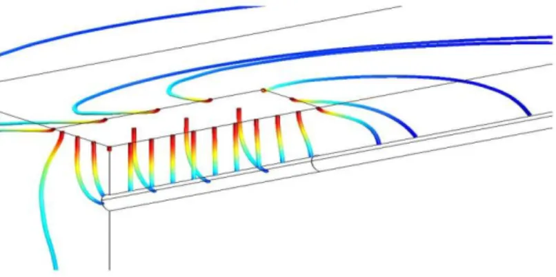
Figures 5 to 9 show current density streamlines resulting from each simulation case implemented in this study. The result in terms of current density streamlines of the first simulation G1CE is shown in Fig.5. It can be observed that much of the

injected current does not polarize the target zone Sp since many current lines spread

out of this area. The numerical experiment allows the amount of current ISp actually

collected by the target zone to be calculated quite exactly. It is computed by integrating local current densities acting on Sp. Table 3 presents a comparison

between the injected current ICE and the collected current ISp. Observations made on

Figure 5. Current density streamlines : G1CE

When a guard ring is used (Fig.6), the current injected by CE appears more confined, especially in the rebar longitudinal plane. However, in the rebar transversal plane, some current lines from CE do not end on the target zone, indicating a slight under-confinement. Table 3 confirms this observation since 92 % of ICE is collected

on Sp.

Figure 6. Current density streamlines : G1

Table 3. Current injected by CE and actually collected by the surface Sp

Simulation case Comment _(μA) I _(μA) I I / I (%) G CE only 8.04 2.65 33 G CE + GR 4.87 4.48 92 G E -E axis parallel 4.88 6.64 136 G E -E axis perpendicular 4.88 4.68 96 G Rectangular CE 19.28 10.96 57

For the probe G2, two simulations were carried out according to the E1-E2 axis

orientation. When the E1-E2 axis was parallel to the rebar axis (noted G2par), good

confinement was observed in the rebar direction (Fig.7). As is often represented in the literature by two-dimensional illustrations, streamlines from CE extended approximately to the middle of the space between CE and GR. However, in the plane perpendicular to the rebar, some current lines from GR ended on Sp, resulting in

over-confinement. The consequence was that the steel surface Sp considered for Rpa

calculation collected more current than assumed, about 36% as indicated in table 3. In contrast, in the case where the E1-E2 axis was perpendicular to the rebar (noted

G2per), a few current lines injected by CE were lost (Fig.8), meaning that the injected

current was slightly under-confined (about 4 % as indicated in table 3).

Figure 7. Current density streamlines : G2par

Therefore, a first conclusion can be drawn here about the significance of E1-E2

positioning regarding the effectiveness of the confining device. Moreover, the global confinements achieved for cases G1 and G2per were similar, 92 % and 96 %

respectively. These values express slight under-confinements and could be considered as satisfactory, but the developments below will show that this condition is actually not sufficient.

The use of annular probes to assess the corrosion rate of linear steel bars leads to complex three-dimensional effects in the current density distribution. Fig. 9 shows the current distribution related to probe G3, which was simply rectangular. Since

there was no confinement device, some current density streamlines naturally spread all over the concrete volume. Table 3 shows that only 57 % of the injected current was collected by the steel located under the probe. However, a greater longitudinal uniformity can be observed in the current streamlines starting from the central part of the probe, expressing a simpler current distribution compared to annular probes.

Figure 9. Current density streamlines: G3

Table 4 summarizes Rpa and jcorr (= B / Rpa) values deduced from each simulated

probe by applying the recommended protocol and the true Rp (1.16 ohm.m²) and jcorr

(1.5 μA/cm²) values, which were kept for each simulation case. The table also presents the local current density Δil actually polarizing the point where the potential

shift ΔE is considered (top of the rebar under the centre of the probe) for each case and the average current density Δia resulting from the application of RILEM

recommendations.

As expected, the average current density Δia was systematically different from the

local current density Δil, due to the real three-dimensional nature of the physical

problem. This resulted in a systematic mis-estimation of Rp since the local current

corresponding to the shift ΔE was not well approximated by the average current. Moreover, it was observed that the satisfactory global confinements achieved for G1

and G2per were not sufficient to correctly assess the value of Rp since the

recommended protocol does not take the three-dimensional distribution of the polarizing current into account. This was particularly demonstrated by the fact that,

although the best confinement was achieved for G2per (96 % versus 92 % for G1), the

best estimation of Rp was obtained for the G1 configuration, only because of

geometrical effects. The G1 simulation case provided an Rp value that was

overestimated by +21 %, while Rp was overestimated by +32 % according to the

G2per configuration. Moreover, it is interesting to note that the G3 simulation resulted

in an underestimation (-26 %), which was in the same error range as G1 and G2per,

whereas no confinement system was used. Regarding the G2 geometry, the

significance of E1-E2 axis positioning was also highlighted for Rp estimation since,

due to the strong over-confinement of 36 %, the G2par simulation resulted in an

overestimation of Rp by +71 % compared to +32 % for G2per.

G G G G G Δi (μA/cm²) 0.22 0.26 0.27 0.21 0.23 Δi (μA/cm²) 0.43 0.21 0.16 0.16 0.31 R (ohm.m²) 0.57 1.40 1.98 1.53 0.85 R (ohm.m²) 1.16 Error on R estimation (%) -51 + 21 + 71 + 32 -26 Estimated j (μA/cm²) 3.05 1.24 0.88 1.14 2.04 Actual value of j (μA/cm²) 1.5 Error on j estimation (%) + 103.2 -17.3 -41.5 -24.3 + 36.2 Table 4. Rp and jcorr estimations and errors

In terms of corrosion rate assessment, table 4 also shows jcorr estimations deduced

from Rpa and B (17.37 mV) values according to Eq.1. The best estimate was

achieved by the G1 configuration and actually corresponded to a significant

underestimation of jcorr (about -17 %). Moreover, it can be observed that the G2per

configuration provided a better estimation of the corrosion rate than the G3

configuration whereas the relative error on Rp estimation was smaller for G3. This

result was simply due to the mathematical form of Eq.1, which gave stronger influence to Rp negative errors than to Rp positive errors. For example, it can be seen

that, despite a strong over-estimation of Rp by +71 %, the G2par configuration gave

smaller errors on the jcorr estimation (about -41 %).

The simulation results show that, even in very favorable conditions (no ohmic drop effects, homogeneous materials, etc.), the recommended protocol for on-site LPR measurement failed to precisely assess the corrosion rate. This was mainly due to the actual non-uniform distribution of the polarizing current in both longitudinal

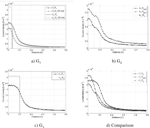
and orthoradial rebar directions, which is not considered by the usual protocols. Fig.10 presents the longitudinal distribution of the polarizing current density computed on the top of the rebar for the different configurations simulated. The dashed line symbolizes the average current (Δia) assumed to polarize the steel rebar

uniformly according to RILEM recommendations.

a) G b) G

c) G d) Comparison

Figure 10. Longitudinal distribution of the current density polarizing the top of the

rebar

It can be observed for all the configurations that current density is maximal under the center of the probe and decreases strongly along the rebar axis, except for G3

where some longitudinal uniformity is observed around the center of the probe as mentioned regarding Fig.9. In cases of high under-confinement (G1CE, G3), the

average current density is significantly higher than the local value of polarizing current density under the center of the probe (Δil). However, in cases of slight global

under-confinement (G1 and G2per), the local value of the polarizing current is still

higher than the average current due to the non-uniform distribution. This result shows that global under-confinement may be partially compensated by the uniform distribution of the polarizing current density. On the other hand, the non-uniform distribution may enhance over-confinement effects (G2par).

Fig.11 was drawn to help the comprehension of the three-dimensional distribution of the polarizing current resulting from the numerical experimentation. The representation is limited to the extension of the polarized surface Sp involved in

the calculation of the apparent polarization resistance Rpa. It can be clearly seen that

the polarizing current distribution is not uniform in the longitudinal direction, nor in the orthoradial direction. Under the center of CE, the current density is about 0.21 μA.cm-2 _{at the top of the rebar while it is about 0.13 μA.cm}-2 _{at the bottom, showing}

that the polarization is much greater on the top of the rebar. The white dotted line links the points where the current density equals the average current density Δia. It

clearly shows that the current density (Δia) involved in Rp estimation is actually not

the current density (Δil) polarizing the point of the rebar where the potential response

is collected, i.e. under the center of the probe.

Figure 11. Distribution of the polarizing current density on Sp for G2per

5. Conclusion

The Linear Polarization Resistance (LPR) technique is being more and more frequently used to assess the corrosion rate of steel reinforcements in concrete. To explain the lack of reliability that is often observed experimentally, numerical simulations were performed in order to improve the physical comprehension of the LPR technique. Several measurement devices using annular and rectangular probe geometries were simulated and the numerical experimentation allowed the relevance of RILEM recommendations to be tested for on-site measurements. Interesting conclusions were drawn based on these numerical experiments.

By drawing polarizing and confining current density streamlines resulting from the simulations, it was shown that the LPR measurement using annular counter-electrodes with confining devices was a real three-dimensional physical problem. Moreover, it was found that some complexity was induced by the use of guard-rings. For example, if complementary reference electrodes (E1 and E2) were used to control

with respect to rebar axis. An optimal configuration was found by positioning the E1

-E2 axis perpendicular to the rebar axis, providing a slight global under-confinement.

If the E1-E2 axis was positioned parallel to the rebar axis, strong over-confinement

was produced.

However, although the confining devices succeeded in limiting global current spreading in some geometrical configurations, the distribution of the polarizing current density at the steel surface was clearly not uniform in either the longitudinal or the orthoradial direction. The major consequence is that the assumption of an average current density uniformly polarizing the steel surface is not relevant, and the calculated LPR, deduced from this assumed current density, is wrong. Regarding the optimal configuration highlighted in this numerical study, although the global confinement was almost perfect, the polarization resistance, assessed according to RILEM recommendations, was still overestimated by more than 20 % and the corrosion rate was underestimated by about 17 %. This error generated by applying RILEM recommendations was due to the existence of a local maximum of the polarizing current distribution which was not taken into account by the protocol. This local current maximum effect compensates the under-confinement and enhances the over-confinement. To improve the RILEM protocol, efforts should be made towards a better estimation of the current density which actually polarizes the point of the rebar where the potential response is collected.

These results also raise some questions about the relevance of the annular geometry of the probes usually used for on-site LPR measurement. For example, the rectangular counter-electrode experimented in this numerical study presented a more uniform current distribution along the rebar axis, indicating a probably easier interpretation although there was no confinement device. Lastly, to emphasize the true difficulty of real on-site LPR measurements, it has to be recalled that these results, highlighting some theoretical limits of the usual protocol, were achieved from numerical simulations carried out in very favorable conditions: stationary measurement, no ohmic drop, uniform corrosion, homogeneous materials, etc. This study focused on geometrical effects but complementary research is currently being conducted to understand the effects of the various other influential factors and thus to improve measurement protocols.

4. References

Feliu S., González J.A., Andrade C., « Effect of Current Distribution on Corrosion Rate Measurements in Reinforced Concrete », Corrosion, vol. 51, n° 1, 1995, p. 79-86 Gepraegs O.K., Hansson C.M., « A comparative evaluation of three commercial instruments

for field measurements of reinforcing steel corrosion rates », Journal of ASTM

International, vol. 2, n° 8, 2005, p. 1-16.

Gulikers J., « Theoretical considerations on the supposed linear relationship between concrete resistivity and corrosion rate of steel reinforcement », Materials and Corrosion, vol. 56, n° 6, 2005, p. 393-403.

Gulikers J., Raupach M., « Numerical models for the propagation period of reinforcement corrosion - Comparison of a case study calculated by different researchers », Materials

and Corrosion, vol. 57, n° 8, 2006, p. 618-627.

Janusz F., in: Condition evaluation of concrete bridges relative to reinforcement corrosion - Vol.2: Method for measuring the corrosion rate of reinforcing steel, Strategic Highway Research Program, Washington DC, 1993.

Kranc S.C., Sagües A.A., « Polarization current distribution and electrochemical impedance response of reinforced concrete when using guard ring electrodes », Electrochimica Acta, vol. 38, n° 14, 1993, p. 2055-2061.

Liu Y., Weyers R.E., « Comparison of guarded and unguarded linear polarization CCD devices with weight loss measurements », Cement and concrete research, vol. 33, n° 7, 2003, p. 1093-1101.

Nasser A., Clément A., Laurens S., Castel A., « Influence of steel–concrete interface condition on galvanic corrosion currents in carbonated concrete », Corrosion Science, vol. 52, n° 9, 2010, p. 2878-2890.

Nygaard P.V., Geiker M.R., Elsener B., « Corrosion rate of steel in concrete: evaluation of confinement techniques for on-site corrosion rate measurements », Materials and

Structures, vol. 42, n° 8, 2009, p. 1059-1076.

Poupard O., L‟Hostis V., Laurens S., Catinaud S., Petre-Lazar I., « Benchmark des Poutres de la Rance”: Damage diagnosis of reinforced concrete beams after 40 years exposure in marine environment by non destructive tools », Proceedings of the EUROCORR 2005

conference, Lisbon, 4-8 September, 2005.

Raupach M., « Models for the propagation phase of reinforcement corrosion - an overview »,

Materials and Corrosion, vol. 57, n° 8, 2006, p. 605-613.

RILEM Technical Committee 154 EMC (Andrade C., Alonso C., Gulikers J., Polder R., Cigna R., Vennesland O., Salta M, Raharinaivo A., Elsener B.), « Test methods for on-site corrosion rate measurement of steel reinforcement in concrete by means of the polarization resistance method », Materials and Structures, vol. 37, n° 273, 2004, p. 623-643.

Song G., « Theoretical analysis of the measurement of polarisation resistance in reinforced concrete », Cement and Concrete Composites, vol. 22, n°, 2000, p. 407-415.

Stern M., Geary A.L., « Electrochemical polarization», Journal of the electrochemical

society, vol. 104, n° 1, 1957, p. 56-63.

Tang L., Fu Y., « A rapid technique using Handheld instrument for mapping corrosion of steel in reinforced concrete », Restoration of Buildings and Monuments, vol. 15, n° 5/6, 2006, p. 387-400.

Warkus J., Raupach M. and Gulikers G., « Numerical modelling of corrosion - Theoretical backgrounds », Materials and Corrosion, vol. 57, n° 8, 2006a, p. 614-617.

Warkus J., Raupach M., « Modelling of reinforcement corrosion - Corrosion with extensive cathodes », Materials and Corrosion, vol. 57, n° 12, 2006b, p. 920-925.

Wojtas H., « Determination of corrosion rate of reinforcement with a modulated guard ring electrode; analysis of errors due to lateral current distribution », Corrosion Science, vol. 46, n° 7, 2004, p. 1621-1632.