HAL Id: tel-02161866
https://hal.archives-ouvertes.fr/tel-02161866v2
Submitted on 15 Oct 2019HAL is a multi-disciplinary open access archive for the deposit and dissemination of sci-entific research documents, whether they are pub-lished or not. The documents may come from teaching and research institutions in France or abroad, or from public or private research centers.
L’archive ouverte pluridisciplinaire HAL, est destinée au dépôt et à la diffusion de documents scientifiques de niveau recherche, publiés ou non, émanant des établissements d’enseignement et de recherche français ou étrangers, des laboratoires publics ou privés.
Luke Bertot
To cite this version:
Luke Bertot. Improving the simulation of IaaS Clouds. Data Structures and Algorithms [cs.DS]. Université de Strasbourg, 2019. English. �NNT : 2019STRAD008�. �tel-02161866v2�
Université de Strasbourg
École doctorale Mathématiques, Sciences
de l’Information et de l’Ingénieur
Laboratoire ICube
THÈSE
présenté par :Luke Bertot
Soutenue le : 17 Juin 2019
pour obtenir le grade de : Docteur de l’université de Strasbourg Discipline / Spécialité : Informatique
Improving the simulation
of IaaS Clouds.
Amélioration de simulation de cloud IaaS via l’emploi de méthodes stochastiques.
THÈSE dirigée par :
Stéphane GENAUD, professeur des universités, université de Strasbourg
Co-Encadrant :
Julien GOSSA, maitre de conférences, université de Strasbourg
Rapporteurs :
Laurent PHILIPPE, professeur des universités, université de Franche-Comté Christophe CÉRIN, professeur des universités, université Paris XIII
Autres membres du jury :
Acknowledgments
Some experiments presented in this thesis were carried out using the Grid’5000 exper-imental testbed, being developed under the INRIA ALADDIN development action with support from CNRS, RENATER and several Universities as well as other funding bodies (see https://www.grid5000.fr).
Contents
Acknowledgements i Contents iii Introduction vii Motivations . . . vii Contribution . . . viii Outline . . . viiiI
Background
1
1 Context 3 1.1 Cloud Computing . . . 3 1.2 Scientific Computing . . . 4 1.3 Sample applications . . . 7 1.3.1 OMSSA . . . 7 1.3.2 Montage . . . 92 Operating Scientific workloads on IaaS Clouds 11 2.1 Cloud Scheduling . . . 11 2.1.1 Scaling . . . 11 2.1.2 Scheduling . . . 12 2.1.3 Cloud brokers . . . 12 2.2 Schlouder . . . 13 2.2.1 Schlouder operation . . . 13 2.2.2 Scheduling heuristics . . . 17
3 Simulation of IaaS Clouds 21 3.1 Simulation technologies . . . 21 3.2 Building a Simulator . . . 23 3.2.1 SimGrid . . . 23 3.2.2 SchIaaS . . . 26 3.2.3 SimSchlouder . . . 27 3.3 Evaluation of SimSchlouder . . . 29 3.3.1 Experiment rationale . . . 29 3.3.2 Simulation Tooling . . . 30 iii
3.3.3 Analysis . . . 32 3.3.4 Results . . . 32 3.4 Take-away . . . 37
II
Stochastic Simulations
39
4 Monte-Carlo Simulations 41 4.1 Motivation . . . 41 4.1.1 Sources of variability. . . 41 4.2 Stochastic simulations . . . 434.2.1 Resolution of stochastic DAGs . . . 43
4.2.2 Monte Carlo Simulations . . . 44
4.2.3 Benefits of the stochastic approach . . . 45
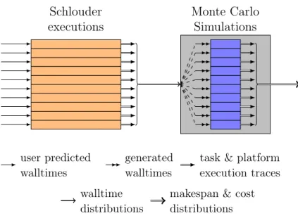
4.3 Our proposed Monte Carlo Simulation . . . 46
4.3.1 Experimental setup . . . 47
4.3.2 Real executions . . . 47
4.3.3 Monte Carlo Simulation tooling . . . 50
4.3.4 Input modeling . . . 51
4.3.5 Results . . . 55
4.4 Take-away . . . 58
5 Defining Simulation Inputs 59 5.1 P: the perturbation level . . . 59
5.2 N: the number of iterations . . . 63
5.2.1 Internal convergence . . . 63
5.2.2 Inter-simulation convergence . . . 66
5.3 Input Distribution Choice . . . 70
5.4 Take-away . . . 72
6 The case of MapReduce 75 6.1 MapReduce and Hadoop . . . 75
6.2 MapReduce simulator MRSG . . . 77 6.2.1 Technical specificities . . . 77 6.2.2 Usage . . . 78 6.3 Experiment . . . 79 6.3.1 Real executions . . . 79 6.3.2 Simulation . . . 81 6.3.3 Discussion . . . 82 6.4 Take-away . . . 84 Conclusion 85 References 87
CONTENTS v
A Résumé en français 93
A.1 Motivations . . . 93
A.2 Contexte . . . 94
A.2.1 Cloud computing . . . 94
A.2.2 Calcul scientifique . . . 95
A.3 Calcul Scientifique dans le Cloud . . . 96
A.3.1 Un planificateur : Schlouder . . . 96
A.3.2 Un simulateur : SimSchlouder . . . 97
A.4 Contributions . . . 97
A.4.1 Simulation de Monte-Carlo . . . 97
A.4.2 Distribution d’entrée . . . 98
A.4.3 Validation expérimentale . . . 99
A.5 Paramétrisation . . . 99
A.6 Le cas Map-Reduce . . . 101
A.7 Conclusion . . . 101
Introduction
Motivations
The recent evolution in virtualisation technologies in the early 2000s has brought about new models for the exploitation of computing resources. These new models, often re-grouped under the umbrella of cloud computing, along with the ever increasing ubiquity of internet access have transformed the hosting and development landscape over the last fifteen years.
Infrastructure as a Service (IaaS) cloud has revolutionized the hosting landscape, by making it possible to provision resources of different sizes on the fly. For hosting providers virtualisation-based provisioning allowed for more homogeneous data-centers and shorter turnaround times on rentals. For users IaaS makes it possible to keep a smaller baseline infrastructure, only raising capacity as necessary, while only paying their actual platform usage.
This new economic model has been hugely successful in the context of service providers, where services are meant to run perpetually and scaling is done to adjust to demand. In the context of finite workloads such as those seen in scientific computing using IaaS clouds poses additional challenges. One such challenge is the need for specialized setups, like in the cases of workloads designed to run on HPC clusters and workloads designed for grids and batch schedulers that are more easily executed on the cloud environments. However such workloads often require external scheduling. Such a scheduler needs to be adapted to the on-demand and the pay-as-you-go nature of IaaS clouds.
On institutional grids and clusters users are usually sheltered from the cost of comput-ing resources. Access policies can range from becomput-ing granted a fixed quota of resources to completely open access. The hidden cost falls on the institution in the form of its invest-ment in infrastructure and manpower. The pay-as-you-go nature of the cloud means that to budget their experiment the user must be able to predict the quantity of computing resources needed. Moreover if they failed to do so the cloud would allow them to continue using resources while charging them potentially over the expected budget. This is only made harder by the on-demand nature of the cloud which allows for different scheduling approaches, some of which have non-trivial impact on workload execution time or cost.
Enabling scientists to use the IaaS cloud to execute scientific workloads will require:
A Cloud Scheduler capable of handling the workloads and managing the cloud
sources for the users. Such a tool must be able to schedule the workload to the cloud as well as provisioning and releasing cloud resources. Doing so automatically diminishes the risk of mismanagement resulting in higher costs.
A Prediction Tool capable of offering an estimate of the cost of executing a workload. This tool must be able to take into account the different available scheduling strate-gies to give the user the opportunity to choose the strategy meeting their needs.
Contribution
This work deals with the problem of building reliable prediction tools. We aim to build such a tool using IaaS cloud simulators. As with other distributed systems, a number of cloud simulation toolkits have been developed. Our team has long worked to evaluate the effectiveness of such simulators as prediction tools. We performed comparisons of real ex-ecutions in different clouds and their corresponding simulations to find which parameters have the biggest impact on simulation precision.
This approach was successful in creating simulations that very closely reproduce their corresponding runs. However the use of such simulations as a prediction tool is still impeded by the inherent variability in the execution of applications on distributed systems such as Infrastructure as a Service (IaaS) clouds. Executing the same workload multiple times on the cloud will not always give the same execution length or cost. Accounting for this variability is a difficult problem, that most simulators do not address. This lapse not only reduces the user’s confidence in the simulation, but reduces the quality of the information offered to the user.
Our thesis is that using stochastic simulation with a single parameter we can account for the variability observed in the executions of scientific applications on the IaaS cloud. In this work we propose a statistical approach to task scheduling on IaaS clouds. Our simulator accounts for the variability of the underlying cloud through a single parameter and presents the user with distributions of possible outcomes with a high level of confi-dence. This method can easily be used to extend other simulators. We use this method to predictively compare scheduling strategies when executing workloads on IaaS clouds, to help the user choose the strategy that best satisfies their time and cost constraints. We show that our simulator is capable of capturing 90% of real executions.
Outline
In Part I of this work we discuss the recent evolutions of IaaS cloud computing and the different types of scientific workloads. In Section 1.3 we present a couple of scientific workloads we used in our experiments. Chapter 2 presents Schlouder, a cloud broker designed to execute batch jobs on IaaS clouds. In Chapter 3 we present SimSchlouder a simulator built to help Schlouder users find which scheduling heuristic matches their needs. We study SimSchlouder’s accuracy in Section 3.3.
ix
In Part II we propose using stochastic simulations as an improvement on our previous deterministic simulation. Chapter 4 presents our attempt to build one such simulation using the Monte Carlo methods. In Section 4.3 we propose one such simulation, a corre-sponding input model and we evaluate it through an empirical experiment. In Chapter 5 we study more precisely the effect of the Monte Carlo simulation (MCS) variables on the simulation’s precision. And in Chapter 6 we study a case in which our MCS failed to produce satisfactory results and discuss the limits of this approach.
Part I
Background
Chapter 1
Context
1.1
Cloud Computing
In computing virtualisation refers to methods and technologies designed to deviate the execution environment from the real environment in which the execution actually happens. These techniques oppose the virtual environment thus created to the physical existing resources. In this work we concern ourselves with cases where virtualisation is used to split a large physical resource set in smaller virtual ones.
Although virtualisation has been historically associated with high computational over-head, over the last decades the integration of hardware-assisted virtualisation in CPUs has greatly reduced the impact of virtualisation and led to the emergence of new economic and exploitation approaches of computer resources in the form of Cloud computing. In the Cloud computing model, operators make a large pool of resources available on de-mand to users, usually in a pay-as-you-go fashion. Most Cloud offers can be classified in three broad categories. The Software as a Service (SaaS) offers provide a web-application, or a light front-end to a server side application, to their users. The Platform as a Ser-vice (PaaS) cloud is usually built around providing automatic deployment and hosting to user code. Last, Infrastructure as a Service (IaaS), which this works focuses on, pro-vides physical resources such as computing power or storage space to the users. IaaS providers operate large datacenters, containing large servers and storage. The large Phys-ical Machines (PMs) are split between the users by way of Virtual Machines (VMs). VMs constrain the available resources to a subset of the resources present on the PM on which the VM is hosted. A large choice of VM configurations, called flavors, allows the users to build a cluster of the appropriate size for their needs. Within a VM the users have full administrative access. Resources are paid by pre-established intervals, called billing time unit (BTU), that range from the minute to the month, with most operators billing hourly, and any started BTU being billed at full price.
Historically the service provided by IaaS clouds was the purview of hosting providers. Much like IaaS cloud providers, hosting providers operate large datacenters and rent part of their resources piecemeal to users. Both of them allow users to set-up their infrastruc-ture without having to invest in the setting up of a datacenter or a server room, nor in
the additional personnel necessary to maintain and operate such infrastructures. High uptime installations are expensive in infrastructure, with redundant power and cooling systems, and in specialised personnel. This is especially problematic for users whose pri-mary activity does not involve much computer infrastructure. Hosting providers could mutualise such costs creating affordable access to high-availability server-grade hardware. The main difference between the historical hosting solutions and IaaS cloud resides in the granularity of the rental.
Virtualisation has allowed IaaS providers to become more effective hosting providers. Since hosting services rented PMs, they had to possess every machine they rented out. Because of this, hosting providers had to support a lot of heterogeneous hardware to satisfy every users’ needs. Misestimated demands could lead to providers running out of a certain machine type while another type of machine remained unused taking up rack space. Setup times for new rentals could take up to a few days depending on machine availability and rentals were operated on a monthly basis. Since VMs are an arbitrary subset of PM resources, IaaS operators do not need to operate heterogeneous hardware to satisfy user needs. On the contrary IaaS operators are encouraged to run large PMs capable of handling any type VMs the operator provides. This setup maximises VM availability and PM usage. Moreover, the time needed to set up a new VM is much shorter than a PM, meaning as long as the datacenter is not at full capacity providing a new VM is almost instantaneous. This is also what enables the finer grained rental periods (BTUs).
The ability to provision resources on the fly has changed the hosting landscape. Users are now able to face unexpected computational load by changing their infrastructure instantly. Either by upgrading to a more powerful VM, referred to as vertical scaling, or by adding more VMs to the infrastructure, called horizontal scaling. Depending on one’s uses of the cloud, scaling can be used in different fashions. For some users, this can be to try to achieve a high level of service availability, like with a website. Scaling is used in this case to face fluctuation in demand. Whereas previous infrastructure had to be sized to handle the highest expected traffic load, users can now size their infrastructure on baseline traffic only bringing in additional resources during usage spikes. This greatly reduces the cost of keeping the service online for the user. For users using resources for computational purposes, scaling allows for a fine control of parallelization. This can be used to achieve shorter makespans (i.e. the time between the submission of the first task and the completion of the last one) at equal cost.
The advantages in infrastructure efficiency for the providers and usage flexibility for users led to the quick expansion of IaaS clouds. Today most of the historical hosting providers also provide virtualised hosting.
1.2
Scientific Computing
Computers’ ability to deal with large amounts of data and computation has opened a lot of new possibilities in all fields of scientific research. Since most of these computations need not be sequential, parallelization is often used to improve and speed up these
scien-1.2. SCIENTIFIC COMPUTING 5 project overlap diff bgmodel background add gather h j k Montage OMSSA
Figure 1.1: Two types of batch jobs. On the left a workflow (Montage [22]). On the right a bag-of-tasks (OMSSA [21]).
tific workloads. Parallelization can be performed in different fashions depending on the granularity of parallelization and the degree of control wanted.
At one end of the spectrum we find workloads designed for High Performance Comput-ing (HPC). Composed of a sComput-ingle executable or a set of closely linked executables, an HPC application divides the workload into a set of computing tasks. These tasks are assigned to all available resources from the beginning to the end of the run. The tasks, that run in parallel and cooperate (for instance through message passing) are generally instances of a same program parameterized by the resource id the program runs on. HPC is usually done on dedicated hardware, and using programming constructs or languages adapted for parallel computing. Notable constructs and language used for HPC include MPI, often used conjointly with OpenMP and GPGPUs where relevant, or PGAS languages (such as X10 and Chapel). Such programs are often written with specific hardware in mind. Because data is exchanged between different processes at runtime, HPC programs must be executed on every node of the cluster synchronously. Although provisioning hardware similar to an HPC cluster is possible in some IaaS clouds, performance remains noticeably inferior to what can be obtained on a dedicated platform ([37, 42]).
On the other end of the spectrum we find batch jobs. These jobs are composed of sequential tasks designed to be executed independently. We classify these workloads in two categories depicted figure 1.1 :
• bag-of-task workloads have no dependencies between their tasks. The tasks can be executed in any order and with any level of parallelism.
Map
Reduce
Figure 1.2: A typical Map Reduce workflow.
can be the input of another task. This constrains the execution order of tasks, however batch jobs do not require tasks be executed simultaneously. Workflows can be represented as directed acyclic graphs (DAGs) as in figure 1.1.
It is possible to find advanced workflow structures such as cases where some tasks are only executed when their dependencies results meet certain criteria. However such workflows are beyond the scope of this work. We will limit ourselves to cases where the dependencies and tasks do not change during the workflow’s execution.
Batch jobs are designed to be executed on a large array of equipment, therefore code specialisation is limited to multicore usage when applicable. Since batch jobs are some set of separate programs, they need to be externally scheduled to be executed on the available machines. Outside of the data-dependencies in workflow the scheduler is afforded a lot of leeway in whether to parallelise the execution of a batch job or not. These scheduling decisions also depend on the available hardware. Historically batch jobs have been computed on resources belonging to universities or research institutions. Either using idle workstations during the off-hours or by investing into dedicated clusters to treat the jobs for the whole institution. Since the early 2000’s, to face the ever increasing computing power needed, institutions have started mutualizing resources into shared infrastructures termed grids, accessed through specialized schedulers. HPC clusters however are rarely used to execute batch jobs since running non-specialised code is seen a wasteful usage of this very expensive equipment. The use of the external scheduler coupled with tasks capable of running on a wide array of hardware setups makes batch jobs a prime candidate for using IaaS cloud.
HPC workloads and batch jobs are the two ends of a spectrum, and some solutions exist in-between. One notable example of such a middle ground solution is found in Hadoop Map-Reduce jobs. Hadoop Map-Reduce is specialised in a single type of of workflow usually operating on a large input. As shown figure 1.2 a typical Map-Reduce job consists in :
• a large number of Map tasks, independent from one another and each operating on a different part of the input.
• a single Reduce tasks taking the Map’s output as input.
Some variations exist, such as using multiple Reduce tasks when dealing with ex-tremely large datasets, or repeating the whole Map-Reduce process for iterative
applica-1.3. SAMPLE APPLICATIONS 7
tions, for instance frequently found in graph algorithms like Page Rank or shortest path computations. Map-Reduce jobs share characteristics with HPC, such as using a single binary running different functions on the various nodes. It also shares some of the batch jobs characteristics, such as adaptability to heterogeneous hardware. Although map tasks are completely independent, the Reduce tasks tries to collect results of finished maps on the fly to reduce the transmission overhead between the last map task and the reduce task. As with batch jobs, this kind of workload is prime for use of IaaS clouds. In fact some IaaS operators such as Amazon Web Service already propose the rental of preconfigured Hadoop clusters.
1.3
Sample applications
In the context of our work we conducted experiments that required running scientific workloads. To do so we used two applications from different scientific fields with wildly different execution profiles.
1.3.1
OMSSA
The first application we use comes from the field of proteomics. It is a data interpre-tation software called Open Mass-Spectrometry Search Algorithm (OMSSA) [21]. The proteomists and computer scientists of the Hubert Curien Pluridisciplinary Institute in Strasbourg have interfaced OMSSA with a production pipeline called Mass Spectrometry Data Analysis (MSDA), accessed through a web portal [12]. For its users, such a tool automatizes the parallel execution of several OMSSA instances distributed over the EGI grid in the Biomed virtual organization. This results in a higher analysis throughput and allows for large scale high throughput proteomics projects. Our team later ported this grid-based solution to an IaaS-cloud environment.
The tandem mass spectrometry analysis (also known as MS/MS analysis) consists in the fragmentation of peptides generated by enzymatic digestion of complex mixtures of proteins. Thousands of peptide fragmentation spectra are acquired and further interpreted to identify the proteins present in the biological sample. Peak lists of all measured peptide masses and their corresponding fragment ions are submitted to database search algorithms such as OMSSA for their identification. Each spectrum is then searched against a database of proteins. As each search is independent from the others, a natural parallelization consists in making this application a bag-of-task (BoT). The MSDA web portal wraps the different tasks in a workflow that manages data as well as parallel computations. It first copies the appropriate databases to a storage server, then groups the spectra into files to be sent to different computation sites. For each spectra file, a job running OMSSA is created to perform the identification search. All jobs can be run independently on different CPUs. The parallelization grain (i.e., the number of spectra distributed to each CPU) per OMSSA execution is computed by MSDA as a function of the requested resolution and the number of available CPUs.
Use-case Tasks Spectra Input (MB) Output (MB) Runtime (s)(measured)
(per task) mean sd mean sd mean sd
BRS 223 1250 2.6 0.4 3.4 1.6 603.1 54.9 (1.2) (0.8) (355.9) (182.1) BRT 33 10000 16.6 2.4 12.4 1.7 125.9 16.6 HRS 65 1250 1.3 0.2 8.9 5.9 182.3 6.8 (0.4) (0.2) (104.3) (19.3) HRT 34 10000 1.7 0.6 4.1 1.4 9.6 2.3
Table 1.1: Key characteristics of the OMSSA tasks in the different use-cases. Tasks with a lower number of spectra than the indicated one have their input sizes and runtime presented in parentheses.
datasets to use as input of OMSSA. These datasets are used to produce 4 OMSSA use-cases based on input data and OMSSA configuration. As described in the previous paragraph each set is composed of a number spectrometry results, each of which are, for parallelization purposes, split into files containing a given number of spectra. The main OMSSA use-case used in our work is called the BRS. BRS runs the most complete peptide search possible on a low resolution set composed of 33 base spectrometer results. These results are split using a granularity of 1250 spectra per file as recommended by the proteomists. This split results in 6 to 8 files per spectrometer result leading to a total workload of 223 tasks. The input size of tasks processing a full 1250 spectra averages 2.6MB with a standard deviation of 0.4MB, variations in file size comes from the format used to store the results. For the files containing less than 1250 spectra the average size 1.2MB with a 0.8MB standard deviations. The output file size appears not to be correlated to input size. The average output file size is 3.4MB and the standard deviation 1.6M. The execution of the workload on our cloud platform gives us a feel for the distribution of runtimes, with data transfers excluded. The average runtime for tasks possesing the full 1250 of spectra is 603.1s with a standard deviation of 54.9s. File with lower number of spectra average 355.9s with a standard deviation of 182.1s. Taking the workload globally, without any parallelization the complete execution of the 233 tasks would require an average of 35 hours and 10 minutes, of which the communications needed to download input files and upload output files represent less than 1%.
Table 1.1 present all the use-cases available to our team. Execution statistics were collected during executions done on our local platform. The first columns up to Output are constant from one execution to the other, whereas runtime will vary depending on the platform and execution. For BRS and HRS which both use lower numbers of spectra part tasks we measured input size and runtimes separately for tasks that don’t have a full number of spectra to analyse. HRT and BRT have such a high number of spectra per tasks that data are not split into multiple tasks.
1.3. SAMPLE APPLICATIONS 9 project overlap diff bgmodel background add gather
. . .
. . .
h. . .
. . .
j. . .
. . .
kFigure 1.3: Directed Acyclic Graph of the Montage workflow
1.3.2
Montage
The second application comes from the field of astronomy. Montage [22] was developed at the California Institute of Technology (CalTech) with funding from the NASA and the National Science Foundation. Montage was designed from the ground up to be executed on a wide range of infrastructures including grids. The California Institute of Technology operates a web-portal allowing registered users to operate the workflow on a CalTech operated grid.
The composition of image mosaics is essential to astronomers. Most astronomical instruments have a limited field of view and a limited spectral range. This means that large astronomical structures can not be observed in a single shot. Composing a final image of a large astronomical structure will often require fusing images taken at different times, from different places, with different instruments. Although temporality and position are not huge factors in terms of the observed subject, astronomical structures do not usually change overnight and Earth’s displacement is mostly negligible, aligning images from such different places and times requires special tools. The Montage Image Mosaic Toolkit (Montage) is one such tool. To generate such mosaics Montage performs two main calculations, re-projection and background rectification. Re-projection computes for each pixel of each input image pixels of the output image, while compensating for shape and orientation of the inputs. Background rectification aims to remove discrepancies in brightness and background, this helps compensating for differences in observation devices, time of night and ground position. Montage is a workflow of specialized tasks presenting strong data dependencies.
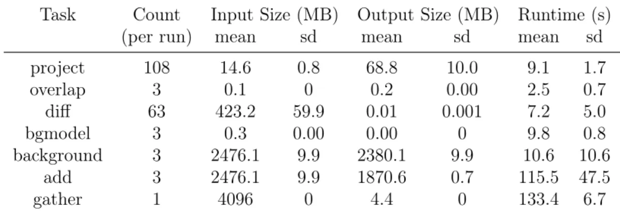
Task Count Input Size (MB) Output Size (MB) Runtime (s)
(per run) mean sd mean sd mean sd
project 108 14.6 0.8 68.8 10.0 9.1 1.7 overlap 3 0.1 0 0.2 0.00 2.5 0.7 diff 63 423.2 59.9 0.01 0.001 7.2 5.0 bgmodel 3 0.3 0.00 0.00 0 9.8 0.8 background 3 2476.1 9.9 2380.1 9.9 10.6 10.6 add 3 2476.1 9.9 1870.6 0.7 115.5 47.5 gather 1 4096 0 4.4 0 133.4 6.7
0: Zero, these inputs and outputs are always the exact same size. 0.00: Non-zero values inferior to the kB.
Table 1.2: Key characteristics of the Montage tasks in our usecase.
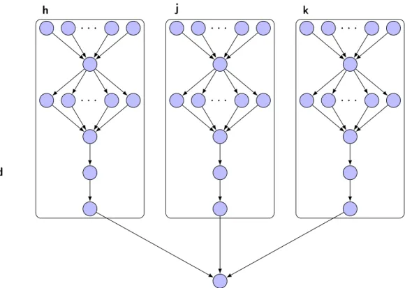
Our dataset for this workflow comes from the 2 Micron All-Sky Survey (2MASS) performed by the University of Massachusetts between 1997 and 2001. This survey was performed on 3 different wavelength bands with a resolution of 2 arc-second. Our workflow only ran on a small sample taken from this extensive sky survey, showing the Pleiades star cluster. The workflow used for our executions of Montage is presented figure 1.3. It can be understood as 3 Montage sub-DAGs fused together at the last step of the workflow. Each sub-DAG works on the images of a different wavelength band, h, j, and k. These bands are well known for their low rate of absorption by atmospheric gasses and are centered on 1.65µm, 1.25µm and 2.17µm respectively. Within the band graphs the project tasks compute the re-projections based on headers contained within the header images. The re-projected images are then sent to an overlap task which computes the overlapping regions of the different re-projected images. These overlapping regions are distributed to diff tasks charged with comparing the overlapping regions on the re-projected images created by project tasks. The comparisons thus created are then used by a bgmodel task to compute the necessary brightness and background corrections for every re-projected image. These corrections are applied to every single re-projected image by the background task. It should be noted that although it is not the case in our setup, the background task can be parallelized in the same fashion as project and diff tasks. The add tasks then splices the different re-projected images in a single mosaic image for the given band. Finally the gather task fuses the mosaics produced for each of the bands.
Table 1.2 provides the distributions of input size, runtime, and output size for the different tasks-types across all executions of Montage. It should be noted that overlap and gather only use as inputs data generated within the workflow. This explains why we found a 0 standard deviation for these input sizes. Conversely bgmodel and gather outputs are also extremely constant. Overall Montage is much more communication intensive, with data transfer times representing between 42% and 64% of task executions depending on the platform parameters.
Chapter 2
Operating Scientific workloads on IaaS
Clouds
2.1
Cloud Scheduling
Our team has been working on the opportunities of using IaaS clouds to execute batch-job like workloads. As defined earlier, clouds are essentially scalable infrastructures. Therefore, executing a workload implies two actions: i) provision an appropriate number of resources, and keeping this number adapted to the intensity of the workload, and ii) map the computations to the resources in a timely manner. Although a small workload could be planned and executed manually by a user, larger workloads will require automation to be properly processed and monitored. Before describing our cloud scheduling system, we quickly define the terms scaling and scheduling, which correspond to actions i) and ii) respectively, as these terms are frequently encoutered in the literature related to clouds.
2.1.1
Scaling
Scaling is the act of provisioning enough resources for one’s workload. Commercial entities and research institutions alike have had to deal with scaling since computers became an essential tool for their activities. The difficulty is striking the balance between acquiring enough resources to fulfill all of their needs without overspending resulting in resources that would sit unused. Cloud computing has not fundamentally changed this core balance at the heart of scaling, but it does offer the user the opportunity to change that balance at any time, as long as they can afford it.
In the prominent field of cloud applications which is web-based applications, scaling is generally the only action that matters. In this field indeed, requests that require processing arrive continuously over time. Therefore, no scheduling of the processing can be anticipated. Given that the requests are independent from one another, scaling is mostly about guaranteeing enough resources are available at any moment to fulfill every request sent to their web service. In such a context a scaling system will usually be concerned with tracking metrics about the overall application load and pro-actively [13,
55] or reactively [15] allow for the adding or removing of resources to the pool. These forms of auto-scaling are available commercially through third party solutions such as RightScale [41] or Scalr [43] or through the cloud operators themselves (e.g. [2]).
The context of finite workload scaling is more about balancing the total runtime of the workload, called the makespan, against a second metric, often the cost or energy requirements. Examples of simple scaling policies designed to minimize the makespan in priority by greedily starting new resources can be found in [53] or [19], while an example of scaling with power consumption minimization can be found in [18].
2.1.2
Scheduling
Scheduling is the act of assigning a task to an available computing resource. Schedulers are at the core in batch-job systems where they were used to split a shared pool of resources between the submitted jobs in a queue. Systems like Condor [51] allowed universities to pool their computing resources into one system that would automatically distribute tasks submitted for execution. Such systems were mainly concerned with the proper repartition of resources and respecting the tasks’ constraints, such as dependencies between different tasks. Such schedulers could be divided into two categories:
• Offline schedulers: which need to know all the jobs to perform and the available resources ahead of time.
• Online schedulers: which accept new jobs on the fly.
In either case schedulers worked within given resources. They could not, as we can in IaaS, provision new resources as needed. The rise of IaaS gave birth to a new class of algorithms combining scaling and scheduling.
2.1.3
Cloud brokers
Cloud brokers are capable of performing both scaling and scheduling in tandem. In some cases these designs were proposed as an extension to a grid scheduler, making it possible to complement local resources by provisioning additional machines from the cloud ([33, 38]). Others fully relied on cloud resources.
PaaS brokers constrain users to their APIs and mask the underlying resources. JCloud-Scale [28] proposed by Leitner et al. lets the user provide constraints to respect during execution. mOSAIC [39] requires the users to provide the tasks’ needs and minimal performance constraints. And Aneka [52] provides a deadline constraint strategy.
IaaS brokers on the other hand provide a more direct access to the underlying resources. IdleCached [49] is a cloud broker that attempts to optimize the cost by scheduling tasks on idle VMs by following an earliest deadline first policy. E-clouds [34] provides off-line schedules of a pre-establish list of available applications. The home-grown project Schlouder [35] lets the user select a provisioning and scheduling heuristic from a library containing strategies optimizing for makespan or for cost.
2.2. SCHLOUDER 13 Schlouder Client Job Description Scheduling Heuristic User Core CloudKit (5)Scheduler Slurm Schlouder Server Cloud Frontend VM VM IaaS cloud (6,8) (7) (1) (2) (4,9) config(10) config(3)
Figure 2.1: The Schlouder cloud brokering system.
2.2
Schlouder
Schlouder, the aforementioned cloud broker, has been developed in our team to schedule batch jobs on IaaS clouds. Schlouder is designed to work with bag-of-tasks and workflows. Schlouder was developed in Perl from 2011 to 2015 by Étienne Michon with contributions from Léo Unbekandt and this author. A functional installation of Schlouder requires a functional installation of Slurm, a job management program service, munge, the au-thentication service used by Slurm, and a DNS service. Schlouder is made available for usage under GPL licence on INRIA’s public forge [45]. This author contributed late to Schlouder’s development helping to provide better logging capabilities and to debug scheduling edge-cases.
2.2.1
Schlouder operation
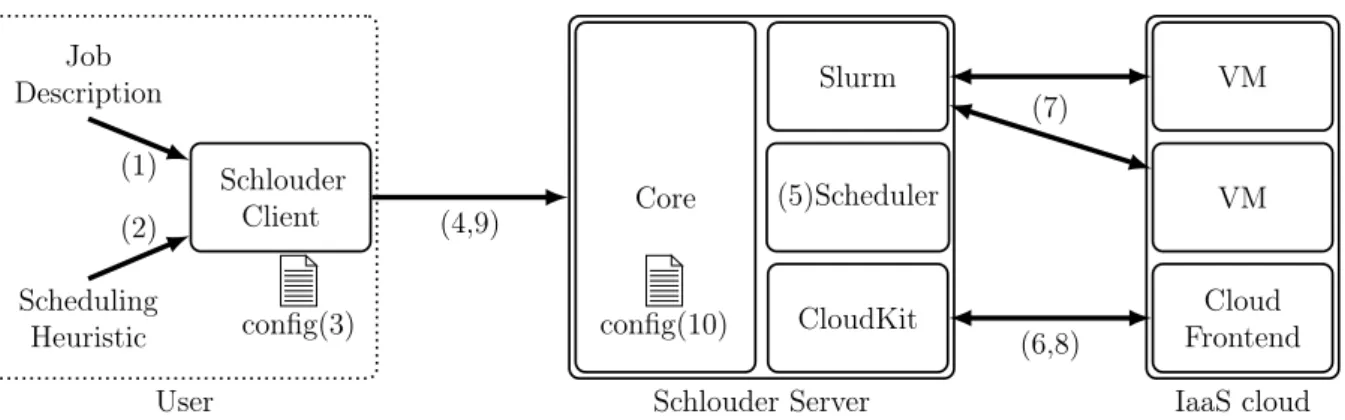
Figure 2.1 offers an overview of Schlouder’s operation.
Client-Side operation. The user interacts with Schlouder through the Schlouder client, shown on the left hand side of the figure. To start the execution of a new workload the user provides:
1. Job description Provided as a lists of scripts. Each script is a single task. The task’s name, expected runtime, and dependencies if any are provided through headers in its script. The rest of the script is executed on the VM when the task is executed.
2. Scheduling Heuristic The user chooses from the heuristics installed on the server which one to use to schedule their workload.
The Schlouder client configuration file (3) provides additional settings such as the pre-ferred instance type and the cloud selection criterion, when applicable, as well as the address and connection parameters to the Schlouder server.
Workload execution. The client sends all this data to the Schlouder server (4). As the server receives data from the client it immediately starts the process of executing the user’s workload.
5. Scheduling is done using the heuristic chosen by the user. The scheduler schedules tasks one at a time as soon as all dependencies are satisfied. Tasks are either scheduled to existing VMs or to a VM to be provisioned.
6. Provisioning is done through the Cloud Kit module. The cloud kit is the inter-face between Schlouder and the cloud by implementing the API calls necessary for Schlouder’s operation. The cloud kits are API dependent, as such multiple clouds using the same API do not require different cloud kits. The functions required by Schlouder are:
• runInstance: provisions a new instance from the cloud.
• instanceIsRunning: determines whether a given instance has successfully booted and reached the running status.
• getIPAddressFromId & getHostnameFromId: these functions are used when pushing tasks to the VMs
• describeInstances: provides a list of all provisioned instances, their current state and IP address when applicable.
• terminateInstance: terminates a specific instance.
Cloud specific configurations must be provided to the Schlouder server for every cloud currently in use. These files contain the cloud kit to use, cloud connection credentials to use, the VM image to use, a list of available instance types, cloud usage quotas if applicable and a boot time prediction model.
7. Task execution Once a VM has been provisioned the tasks queued on it by the scheduler are executed by the task manager, Slurm by default. Slurm copies the task’s script to the VM and monitors the scripts execution. When a task finishes Slurm retrieves the execution log before executing the next queued task.
8. Instance shutdown is done through cloud kit’s terminateInstance function. Shut-downs are only performed when a VM is without any running or queued tasks and it reaches the shutdown margin at the end of its BTU.
9. Client monitoring At anytime during or after the execution the user can use the Schlouder client to monitor the advancement of the execution. The report sent by the server contains the list of all active, shutdown, and planned VMs, and for each of those the list of executed, running, and queued tasks.
Server Configuration. The server configuration(10) contains the necessary informa-tion for Schlouder to operate, including:
• Application setup: Binding address and port, temporary directory, client usernames, BTU length, and shutdown margin.
2.2. SCHLOUDER 15 events time State metrics provisioning decision Future provisioning request Pending VM start Booting Idle jobs assigned Busy shut-down request Shut-down Terminated uptime
boot time jobs walltimes
Figure 2.2: VM lifecycle
• Cloud setup: List of available clouds and for each cloud : – the API to use
– connection information – boot time estimators – usage quotas
– available instance types – disk image to use
• Task manager setup: system to use and configuration file • Scheduler setup: a list of available scheduling heuristics
Although they are part of the application and cloud setup respectively the BTU length (length of the cloud’s billing cycle), the shutdown margin (overhead scheduled for shut-down), cloud usage quotas, and the boot time estimators are also inputs of Schlouder’s scheduler.
VM lifecycle management. From the moment the scheduler decides to provision a new VM Schlouder’s node manager thread creates the internal representation necessary to track its status. Figure 2.2 schematize this lifecycle, its key event and the metrics reported by Schlouder.
1. Future As soon as Schlouder’s scheduler requires a new VM a new task queue is created. The scheduler is made aware of this task queue and immediately able to schedule more tasks to it. The start time/end times of the jobs in the queue are computed on the basis of the boot time estimators and the tasks’ expected runtimes. Internally the tasks is assigned to a VM with the Future state.
2. Pending is the state assigned to a VM for which a provisioning request has been submitted to the cloud. As with the Future state, Pending VMs are simple tasks queues existing mostly to allow the scheduler to continue normal operation. The difference between Future and Pending exists for Schlouder to keep track of how many provisioning requests need to be done and how many VMs are still expected from the cloud.
3. Booting As soon as a new VM resource appears on the cloud it is assigned to the oldest Pending VM. The internal representation of the VM is completed with available information from the cloud and its state is switched to Booting. Schlouder will store the current time as the VM’s start date and the task queue is recomputed using this date to allow for more precise scheduling. Two timers are set, the shutdown timer roughly as long as BTU and the short startup monitoring timer. The latter instructs Schlouder to check if the VM has been detected by Slurm. Becoming visible in Slurm switches the VM to the Idle/Busy states depending on context. The time elapsed in the Booting state is recorded as the boot time. The tasks queue is updated with the measured boot time in place of the boot time estimation.
4. Idle/Busy During normal operation the VMs will alternate between the Idle and Busy state depending on whether they are running any tasks at a given time. Each time a VM finished a given task the task queue is updated to adjust for any deviation for the prediction. This allows the scheduler to always operate on the most precise information available.
5. Shutdown The first shutdown timer of any given VM is setup to trigger one shutdown margin (as indicated in the server configuration) before the end of the BTU. Once the shutdown timer is triggered Schlouder checks whether the VM is Idle and its tasks queue is empty in which case Schlouder will set the VM state to Shutdown and send the corresponding request to the cloud. A VM in the Shutdown state becomes unavailable to the scheduler. VMs which do not meet the shutdown criterion see their shutdown timer extended for 1 BTU.
6. Terminated Schlouder monitors the status of VMs in the Shutdown state until they are removed from the cloud resource list. When this happens the VM’s state switches to Terminated and the current time is stored as the VM’s stop date. The VM’s uptime is computed from the VM’s start date and stop date and added to Schlouder’s output.
Task lifecycle management. Like with node management Schlouder also keeps a task manager thread in charge of tracking the different tasks lifecycle and stores many metrics for review and analysis. The lifecyle of a single task is presented figure 2.3.
1. Pending Tasks received from a client are added to the scheduling queue. The time at which the server receives the tasks is called the submission_date. Newly received tasks are attributed the Pending state.
2. Scheduled Once all the dependencies of the task reach the Complete state the task can be scheduled. Once the scheduler assigns the tasks to a task queue the task’s state is switched to Scheduled. The time at which the scheduling happens is recorded as scheduling_date.
3. Submitted A task will remain in its Scheduled state until its turn to be executed on its assigned node comes up. Once the task is handed over to Slurm for execution
2.2. SCHLOUDER 17 events time State metrics task reception Pending node assigned Scheduled task sent to node Submitted task starts on node
Inputting Running Outputting task ends on node Finished Complete submission_date scheduling_date start_date walltime
inputtime runtime outputtime managementtime
Figure 2.3: Tasks lifecycle
the task is considered Submitted and the current time recorded as the task’s start_date.
4. Once the task is under Slurm’s control Schlouder does very little to track its start and its advancement. However for tasks following the intended format it is possible to report to Schlouder an input_time, runtime, and output_time. These times are retrieved from the task’s execution log and therefore not known by Schlouder. As such the following states exist for research purposes and not as part of the Schlouder internal representation.
• Inputting The task starts executing on the node, and downloads from storage the inputs necessary for its execution.
• Running The task executes its main payload on the inputs. • Outputting Results from the execution are uploaded to storage.
• Finished The task’s script has finished running on the node. But Schlouder has yet to become aware.
5. Complete Schlouder becomes aware that the task has finished. The current time is used in conjunction with the start_date to compute the jobs effective walltime. The task state is set to Complete and the task queue to which it belonged is updated to account for the effective walltime.
All the Schlouder metrics described in the previous paragraphs are defined in table 2.1. Times and dates are provided in seconds and recent versions of Schlouder have a precision of 1 nanosecond.
Although we just explained the general operation of Schlouder, the most important component during the execution of a workflow is the scheduler. This is the component responsible for the ordering the provisioning of new VMs and the placement of tasks.
2.2.2
Scheduling heuristics
Schlouder’s scheduler takes scheduling and provisioning decisions on a task by task basis, scheduling every task with no pending dependencies. Scheduling decisions are informed
Target Name Unit Source
VM
boot_time_prediction s computed from configuration.
boot_time s measured during Booting state.
start_date date logged at the start of Booting state.
stop_date_prediction date based on start_date, BTU length, and task predicted/effective walltime.
stop_date date logged at the start of terminated state.
Task
submission_date date time at which Schlouder first receives a task. scheduled_date date time at which the scheduler selects a VM for
the task.
start_date_prediction date time at which the scheduler expects the task to start.
start_date date time at which a task is handed to Slurm for execution.
walltime_prediction s provided by the user. (effective) walltime s measured by Schlouder.
input_time s provided by the task, the time spent
downloading inputs.
input_size byte provided by the task, the size in bytes of dif-ferent downloaded inputs.
runtime s provided by the task, the time spent in
com-putations.
output_time s provided by the task, the time spent upload-ing results.
output_size byte provided by the task, the size in bytes of the different uploaded outputs.
management_time s Computed by subtracting runtime,
in-put_time, and output_time from the walltime. The management_time represents unmeasurable delays such as the task’s transfer time and the delay between the tasks ending and Schlouder being aware of the termination.
Table 2.1: Schlouder available metrics. All times and date measured in seconds with a precision to the nanosecond.
2.2. SCHLOUDER 19
by the scheduled task’s expected runtime, the active VMs and their runtimes, eventual future VMs and their expected boot-times, and the expected runtimes of jobs already queued to active VMs.
Alogrithm 2.1 (see below) presents the generic algorithm used for scheduling in Schlouder. This algorithm uses the following definitions:
• t the task to schedule. • v an available VM
• V the set of all such VMs
• C the set of candidate VMs for scheduling
The scheduler first determines which available VMs can be used to run the task to schedule. This is done using a heuristic-dependent eligibility test, eligible(). Then if no VM matches the eligibility conditions a new VM is provisioned and the tasks are queued to it. In cases where one or more VMs are deemed eligible a heuristic-dependent select() function is used to select the VM on which to queue the tasks t.
Algorithm 2.1 Generic Schlouder scheduling algorithm
1: procedure Schedule(t) //a new task t is submitted
2: C ← ∅ //C is the set of candidate VMs (C ⊂ V )
3: for v ∈ V do
4: if eligible(v, t) then //Find eligible VMs
5: C ← C ∪ {v}
6: end if
7: end for
8: if C 6= ∅ then
9: v ← select(C) //Select VM amongst eligible
10: else
11: v ← deploy() //Create and run a new VM
12: V ← V ∪ {v}
13: end if
14: enqueue(v, t) //Map the job to the VM
15: end procedure
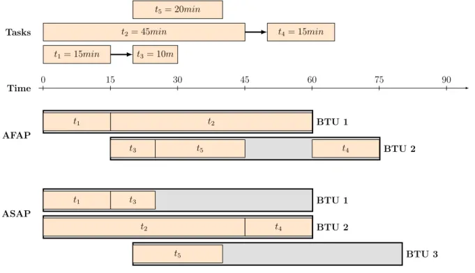
Schlouder is provided with a dozen strategies derived from this generic setup. 1VM4All only ever provisions one VM and represents the worse case scenario in terms of makespan while offering the lower cost of execution. At the opposite end of the spectrum 1VMper-Task immediately schedules every single task on a new VM, therefor offering the shortest possible makespan while being the most expensive heuristic. In this work we will observe Schlouder executions using two heuristics, As Full As Possible (AFAP) and As Soon As Possible (ASAP).
The AFAP strategy aims to minimize the cost of running a workload. As such it will favor delaying tasks to execute them on already running VMs. However since running
Time
0 15 30 45 60 75 90
t5= 20min
Tasks t2= 45min t4= 15min
t1= 15min t3= 10m AFAP BTU 1 t1 t2 BTU 2 t3 t5 t4 ASAP BTU 1 t1 t3 BTU 2 t2 t4 BTU 3 t5
Figure 2.4: Chronograph of the two Schlouder strategies used in this work.
two VMs in parallel has the same cost as running a single VM for two BTUs, AFAP will only consider eligible for scheduling VMs whose expected remaining time can fit the full expected runtime for the task being scheduled. In cases where multiple VMs exists, AFAP will select the best fit.
The ASAP strategy aims to minimize the makespan of a workload. As such it will favor provisioning new VMs over delaying a task’s execution. Therefore it will only consider eligible for scheduling VMs that are already idle at the time of scheduling and VMs that are expected to become idle before an new one can be provisioned. If multiple such VMs exists, ASAP will select best fit.
The expected remaining time of a VM, used in AFAP, is computed using the observed runtime of already executed jobs and the user provided expected runtime of already queued jobs. The expected boot time of a VM is predicted using the parameters provided in the cloud configuration files. These parameters must be estimated, from experience by the operator of the server, and take into account the number of VMs already booting.
Figure 2.4 presents a short example of ASAP and AFAP in a 5-task workload. Tasks t1 to t2 are submitted at the start of the workload with tasks t3 and t4 being dependent on t1 and t2 respectively. Task t5 is submitted separately 20 minutes after the other tasks.
Chapter 3
Simulation of IaaS Clouds
We now have a scheduling tool to execute our workload in the cloud. Experimentation with scheduling shows that for users to choose the correct schedule to fulfill their con-straints is a non-trivial problem. As such, a prediction tool is needed for the user to project the cost and makespan of their workload. We intend to use simulation to provide this prediction.
Simulation has always been a key component of the study of distributed systems. Sim-ulations present three main advantages over experimentations on real platforms. Firstly distributed systems present high installation and maintenance costs, which simulators do not have. Secondly simulations can run experiments faster than real time, allowing to perform lengthy experiments in reasonable times. Lastly, well designed simulations offer an access to the minute-to-minute evolution of systems that are complicated to reproduce, albeit not impossible. However these advantages come at the risk of having the simulation not represent reality. As a gap between the simulation and the corresponding reality is inevitable, if we intend to use simulation for prediction tools we need to establish the deviation between our simulations and reality.
In this chapter we first explore the pervasive principles used in cloud simulation and the available simulation tools. Then we will present the technical solution we used to create a simulator for Schlouder. Finally we will present the evaluation we performed for our simulator and discuss the results’ implications on the use of simulation as a prediction tool.
3.1
Simulation technologies
Discrete event simulations. Most cloud simulators are based on discrete event sim-ulation (DES). A discrete event simsim-ulation is a series of events changing the state of the simulated system. For instance, events can be the start and end of computations or of communications. The simulator will jump from one event to the next, updating the times of upcoming events to reflect the state change in the simulation. A solver, at the core of the DES, considers the system’s states generated by the platform and previous events to
compute the timing of future events. In most cases, simulators have a bottom-up approach: the modeling concerns low-level components (machines, networks, storage devices), and from their interactions emerge the high-level behaviours. Working on disjoint low-level components makes it easier to tune the model’s precision to the wanted accuracy or speed trade-off.
Running a bottom-up DES-based simulator requires at least a platform specification and an application description. The platform specification describes both the physical nature of the cloud, e.g. machines and networks, and the management rules, e.g. VM placement and availability. Depending on the simulator, the platform specification can be done through user code, as in CloudSim [10] for example, or through platform description files, as is mostly the case in SimGrid [14]. The application description consists in a set of computing and communicating jobs, often described as an amount of computation or communication to perform. The simulator computes their duration based on the platform specification and its CPU and network models. An alternative approach is to directly input the job durations extrapolated from actual execution traces.
The available cloud DESs can be divided in two categories. In the first category are the simulators dedicated to study the clouds from the provider point-of-view, whose purpose is to help in evaluating the datacenter’s design decisions. Examples of such simulators are MDCSim [30], which offers specific and precise models for low-level components including the network (e.g. InfiniBand or Gigabit ethernet), operating system kernel, and disks. It also offers a model for energy consumption. However, the cloud client activity that can be modeled is restricted to web-servers, application-servers, or data-base applications. GreenCloud [24] follows the same purpose with a strong focus on energy consumption of the cloud’s network apparatus using a packet-level simulation for network communications (NS2). In the second category are the simulators targeting the whole cloud ecosystem, including client activity. In this category, CloudSim [10] (originally stemming from Grid-Sim) is the most broadly used simulator in academic research. It offers simplified models regarding network communications, CPU, or disks. However, it is easily extensible and serves as the underlying simulation engine in a number of projects (e.g. ElasticSim). Simgrid [14] is the other long-standing project, which when used in conjunction with the SchIaaS cloud interface provides similar functionalities as CloudSim. Among the other re-lated projects, are iCanCloud [36] proposed to address scalability issues encountered with CloudSim (written in Java) for the simulation of large use-cases. Most recently, PICS [23] has been proposed to specifically evaluate simulation of public clouds. The configuration of the simulator uses only parameters that can be measured by the cloud client, namely inbound and outbound network bandwidths, average CPU power, VM boot times, and scale-in/scale-out policies. The data center is therefore seen as a black box, for which no detailed description of the hardware setting is required. The validation study of PICS under a variety of use cases has nonetheless shown accurate predictions.
Alternative approaches to simulations. Although the vast majority of cloud simula-tors are based on bottom-up DESs other approaches are available for creating simulations. One such approach is directed acyclic graph (DAG) computation. This kind of approach is extensively used in project management where methods such as PERT (Program Eval-uation and Review Technique) or Gantt graphs are commonly used to estimate project
3.2. BUILDING A SIMULATOR 23
length. This method works well with the simulation of the types of workflows studied in this work, where tasks have clear ends and defined dependencies, but would not be appropriate for generic cloud simulations. It should be noted that this kind of approach does not preclude the use of a DES, but using PERT methodologies allows one to perform the same simulation from a workflow perspective where the intricacies of the underlying resources are not formalised. Still others build simulators using a top-down approach. Using Trustworthy Simulation to Engineer Cloud Schedulers [40] describes the creation of a simulation model based on perturbation theory. Starting with the most parsimonious model possible, the authors of this work introduce a perturbation in the inputs to repre-sent unmodeled behaviors. If the simulation is insufficiently accurate, terms are added to the main model and the perturbation adjusted in consequence. It should be noted that in this work the simulator using the thus obtained model keeps track of the simulation state using a DES. The originality of this work compared to the ones described in the previous paragraph lies in the use of a top-down model and the use of a perturbation term covering unmodeled behavior.
3.2
Building a Simulator
We designed SimSchlouder as an aptly named simulator for Schlouder executions. Sim-Schlouder is based on SimGrid and uses SchIaaS, a specifically built IaaS simulation extension for SimGrid.
3.2.1
SimGrid
SimGrid [14] is a scientific instrument to study the behaviour of large-scale distributed systems such as Grids, Clouds, HPC, and P2P systems. The SimGrid project was started in 1999 and is still under active development [46].
SimGrid Engine. Simgrid itself is not a simulator but rather a framework and toolkit with which to build DESs. SimGrid provides core functionalities needed for a simulator and a number of user APIs with which to interact with the core functions. Figure 3.1 schematizes the internal structure of the SimGrid toolkit. The key components are:
• XBT contains all the base data-structures and memory handling functions. Written in C this module helps guarantee the portability of SimGrid-based simulators. • SURF is the solver at the core of the SimGrid simulations. Using the platform
representation this module computes the timing of events within the DES.
• SIMIX is a kernel handling the usercode and acts as an application description. The processes handled by SIMIX are executed or suspended in accordance with the timings and events computed by SURF.
• User APIs The remaining modules represent the APIs used by the user creating a simulation based on SimGrid.
SimGrid
XBT(grounding feature, data structures, portability) SURF
(virtual platform simulator) SIMIX
(usercode handling) MSG
CSP API
SMPI run MPI apps in
virtual platform SimDag
simulate DAGs of parallel tasks
Figure 3.1: SimGrid Architecture
– MSG allows the user to represent the simulation content to be presented as Communicating Sequential Processes (CSP). When using MSG the usercode describes a sequence of communications and computations performed by the simulated process.
– SMPI also simulates the application as a set of concurrent processes, but the simulated processes are generated automatically from an existing C or Fortran MPI enabled application. SMPI provides an additional runtime for MPI-specific functionalities.
– SimDAG does not use concurrent processes as a representation of the simu-lated workload but instead allows for an abstract representation as a directed acyclic graph of communicating computational tasks.
Simulations using MSG. Our work relies on the MSG API. This API is available in C, C++, Java, Ruby, and Lua. Writing a simulator with MSG requires the user to provide:
• Simulator code as SimGrid is merely a framework. The user must write a code to instantiate the SimGrid engine and configure it properly before starting the sim-ulation itself.
• Platform file provides a description of the simulated environment within which the simulation happens. It mainly consists in a description of available machines, called hosts, and the networks to which they are connected. SimGrid’s platform syntax offers a wide array of options such as cluster, CPU speed, CPU power consumption, network bandwidth and latency. A number of parameters can be replaced by files
3.2. BUILDING A SIMULATOR 25
that allow the user to vary the parameters along the simulation, e.g. allowing for a simulation where the bandwidth of a link changes over time.
• Usercode representing the actions undertaken by the simulated processes. This code is compiled with the simulator code and will be executed during the simulation at the will of the SIMIX kernel. The usercode uses specific MSG function calls to indicate to the simulator that the simulated process is performing a specific action such as communicating or computing a certain amount of data. Using code to represent the simulated application allows the simulation to react to simulated events in a way static representations can not. In our case usercode allows us to implement task scheduling within the simulation.
• Deployment file indicates to SimGrid on which host of the simulated platform the different simulated processes are executed. This is optional as pinning processes to a host can also be done in the simulator code directly.
A well coded simulator first initialises the SimGrid engine with the MSG user API. Second, the platform file is passed to the engine. Third, simulated processes are set up, either through manual calls to MSG or by passing the deployment file. In this step SIMIX acquires pointers to the usercode to execute during the simulation. Finally the MSG_run function is called to start the simulation.
During the simulation code execution is controlled by the SIMIX kernel. While the simulated processes are running the simulation’s clock is suspended. A simulated process is suspended when it makes an MSG call and the event corresponding to that call is added to the simulation’s timeline. Once all the processes are suspended SURF solves the timing of all the events on the timeline. The simulation’s clock in then advanced to the next event on the timeline and the process suspended by the corresponding call is awaken. The simulator continues alternating between the execution of usercode and the computation of the timeline until all usercode is terminated. At which point the simulation ends and control is handed back to the simulator code.
IaaS cloud within SimGrid. SimGrid is a lower level toolkit to build simulations of distributed systems. Its bottom-up design means SimGrid concerns itself with hosts, their cores, their network interfaces, and the sharing of those resources between the processes working on the hosts. Because of this SimGrid by itself offers very little in terms of tools for cloud simulation. It does however offer one critical element, the ability to partition a host’s resources into simulated VMs. From a functionality perspective the VM interfaces available in MSG matches the functionality expected of an hypervisor kernel module. That is the ability to create of VM based on a number of available physical resources, the ability to start suspend or shutdown this simulated VM, and the ability to assign simulated processes to the VM instead of the underlying host. SimGrid VMs are heavily abstracted and do not have boot or shutdown times. In order to build our simulation of Schlouder we needed to extend the base provided by SimGrid into a proper cloud simulation.
MSG
SCHIaaS Core
Compute Engine
Scheduler
Storage Engine
Load Injector SimSchlouder User Made App
T
racing
Mo
dule
: Replaceable modular elements
Figure 3.2: SchIaaS Architecture
3.2.2
SchIaaS
We designed SchIaaS to provide a tool to build extendable IaaS simulations. SchIaaS is written in Java and works with the Java MSG API. SchIaaS was designed and written as part the ANR project SONGS (Simulation Of Next Generation Systems) of which SimGrid was also part and is available at [44]. Like SimGrid, SchIaaS is designed as a toolkit that is not a simulator by itself but an extension of the of the calls available in MSG. SchIaaS is not however a patch to SimGrid, it rests on top of MSG and SchIaaS call modify the simulation state by a series of coordinated calls to the MSG interface.
Structure. SchIaaS was designed to facilitate both simulations of IaaS clouds and simu-lations of applications using IaaS clouds. Figure 3.2 presents an overview of the structure of SchIaaS. Key elements are as follows:
• SchIaaS core contains the base code for initialisation and loading of modules. • Compute Engine this component contains the code pertaining to VM lifecycle
management. Although a compute engine is provided with the base installation of SchIaaS, this module can be replaced for experiments not compatible with the base implementation.
– Scheduler this component determines on which hosts the VMs are placed on. Because this component is often the subject of independent studies this element can be swapped independently from the standard Compute engine. The SchIaaS installation provides a couple of different schedulers.
• Storage engine this component provides a bucket storage element, with the ability to put and get data from a storage service. This element is replaceable to allow for experimentation with data management.
3.2. BUILDING A SIMULATOR 27
• Tracing module designed to help users extract useful information from the simulated environment.
• Load injector performs simulated VM startup and shutdown requests following user provided pattern or traces. This module is useful for users trying to study behaviours of the cloud itself rather than an application using the cloud.
The last usercode presented in Figure3.2 is our simulator SimSchlouder described here-after.
Functionality. The functions provided by SchIaaS mirrors what is expected of a cloud API. Where SimGrid provides very basic hypervisor level functionalities to control the simulations of VMs, SchIaaS deals in cloud instances. Using SchIaaS the simulated pro-cesses can query available images and instance types, and run, suspend, resume, or ter-minate instances of the required type. Upon request, SchIaaS will provide the underlying simulated VM to the usercode to allowfor the allocation of new simulated processes. Additionally the storage interface allows the simulated processes to trigger uploads and downloads from the dedicated storage nodes.
Usage. To use SchIaaS within a simulation the user must initialise the SchIaaS com-ponent during startup after initialising MSG and loading the platforms. Initialisation is configured by a cloud file. This file describes the simulated clouds. For each cloud the file indicates the Storage and Compute engine, the scheduler, the compute nodes, and the available flavors and disk images. During the simulation simulated processes can make calls to SchIaaS engine functions. These functions are executed as usercode but them-selves make calls to the appropriate MSG functions triggering the events corresponding to the operations of the simulated IaaS cloud.
3.2.3
SimSchlouder
SimSchlouder is a simulation of Schlouder built on top of SimGrid and SchIaaS. It can be found in the SchIaaS repository ([47]). SimSchlouder was first designed as a prediction module for Schlouder, with the objective of offering to the users a preview of the makespan and costs to expect depending on their chosen strategy. Although a prediction module would have to strictly use the same inputs as Schlouder, we quickly extended SimSchlouder to be a general purpose Schlouder simulator with multiple possible levels of inputs. This evolution has helped us make SimSchlouder more accurate, as we will see in Section 3.3, and on occasions has lead finding bugs in Schlouder itself.
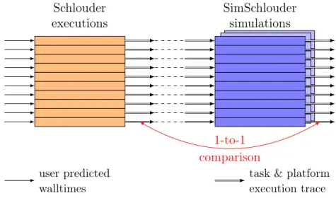
Usage. SimSchlouder runs a simulation of a given platform with a specified cloud. The simulation encompasses the target cloud with its physical components and the Schlouder server with its physical host. The Schlouder-client and its communication with the Schlouder-server are not part of the scope of the simulation. In a run of SimSchlouder
![Figure 1.1: Two types of batch jobs. On the left a workflow (Montage [22]). On the right a bag-of-tasks (OMSSA [21]).](https://thumb-eu.123doks.com/thumbv2/123doknet/14283551.491889/18.892.158.771.126.511/figure-types-batch-workflow-montage-right-tasks-omssa.webp)