HAL Id: hal-01620848
https://hal.archives-ouvertes.fr/hal-01620848
Submitted on 21 Oct 2017
HAL is a multi-disciplinary open access
archive for the deposit and dissemination of
sci-entific research documents, whether they are
pub-lished or not. The documents may come from
teaching and research institutions in France or
abroad, or from public or private research centers.
L’archive ouverte pluridisciplinaire HAL, est
destinée au dépôt et à la diffusion de documents
scientifiques de niveau recherche, publiés ou non,
émanant des établissements d’enseignement et de
recherche français ou étrangers, des laboratoires
publics ou privés.
Efficient Optimal Ate Pairing at 128-bit Security Level
Md Al-Amin Khandaker, Yuki Nanjo, Loubna Ghammam, Sylvain Duquesne,
Yasuyuki Nogami, Yuta Kodera
To cite this version:
Md Al-Amin Khandaker, Yuki Nanjo, Loubna Ghammam, Sylvain Duquesne, Yasuyuki Nogami, et
al.. Efficient Optimal Ate Pairing at 128-bit Security Level. IndoCrypt 2017 - 18th International
Conference on Cryptology, Dec 2017, Chennai, India. pp.186-205. �hal-01620848�
Efficient Optimal Ate Pairing at 128-bit Security
Level
Md. Al-Amin Khandaker1( )[0000−0001−7330−138X], Yuki Nanjo1, Loubna Ghammam2, Sylvain Duquesne3[0000−0002−3854−8253], Yasuyuki Nogami1[0000−0001−6247−0719], and Yuta Kodera1[0000−0002−6482−6122]
1
Faculty of Engineering, Okayama University, 7008530, Okayama, Japan {khandaker,yuki.nanjo,yuta.kodera}@s.okayama-u.ac.jp,
2 Normandie Universit´e, UNICAEN, ENSICAEN, CNRS, GREYC,
14000 Caen, France [email protected]
3
Univ Rennes, CNRS, IRMAR - UMR 6625, F-35000 Rennes, France [email protected]
Abstract. Following the emergence of Kim and Barbulescu’s new num-ber field sieve (exTNFS) algorithm at CRYPTO’16 [21] for solving dis-crete logarithm problem (DLP) over the finite field; pairing-based cryp-tography researchers are intrigued to find new parameters that con-firm standard security levels against exTNFS. Recently, Barbulescu and Duquesne have suggested new parameters [3] for well-studied pairing-friendly curves i.e., Barreto-Naehrig (BN) [5], Barreto-Lynn-Scott (BLS-12) [4] and Kachisa-Schaefer-Scott (KSS-16) [19] curves at 128-bit secu-rity level (twist and sub-group attack secure). They have also concluded that in the context of Optimal-Ate pairing with their suggested param-eters, BLS-12 and KSS-16 curves are more efficient choices than BN curves. Therefore, this paper selects the atypical and less studied pairing-friendly curve in literature, i.e., KSS-16 which offers quartic twist, while BN and BLS-12 curves have sextic twist. In this paper, the authors op-timize Miller’s algorithm of Optimal-Ate pairing for the KSS-16 curve by deriving efficient sparse multiplication and implement them. Further-more, this paper concentrates on the Miller’s algorithm to experimentally verify Barbulescu et al.’s estimation. The result shows that Miller’s al-gorithm time with the derived pseudo 8-sparse multiplication is most efficient for KSS-16 than other two curves. Therefore, this paper defends Barbulescu and Duquesne’s conclusion for 128-bit security.
Keywords: KSS-16 curve, Optimal-Ate pairing, sparse multiplication
1
Introduction
Since the inception by Sakai et al. [25], pairing-based cryptography has gained much attention to cryptographic researchers as well as to mathematicians. It gives flexibility to protocol researcher to innovate applications with provable
security and at the same time to mathematicians and cryptography engineers to find efficient algorithms to make pairing implementation more efficient and practical. This paper tries to efficiently carry out the basic operation of a specific type of pairing calculation over certain pairing-friendly curves.
Generally, a pairing is a bilinear map e typically defined as G1× G2→ GT,
where G1 and G2 are additive cyclic sub-groups of order r on a certain elliptic
curve E over a finite extension field Fpk and GT is a multiplicative cyclic group
of order r in F∗pk. Let E(Fp) be the set of rational points over the prime field
Fp which forms an additive Abelian group together with the point at infinity
O. The total number of rational points is denoted as #E(Fp). Here, the order r
is a large prime number such that r|#E(Fp) and gcd(r, p) = 1. The embedding
degree k is the smallest positive integer such that r|(pk−1). Two basic properties
of pairing are
– bilinearity is such that ∀Pi∈ G1and ∀Qi∈ G2, where i = 1, 2, then e(Q1+
Q2, P1) = e(Q1, P1).e(Q2, P1) and e(Q1, P1+ P2) = e(Q1, P1).e(Q1, P2),
– and e is non-degenerate means ∀P ∈ G1 there is a Q ∈ G2 such that
e(Q, P ) 6= 1 and ∀Q ∈ G2there is a P ∈ G1such that e(P, Q) 6= 1.
Such properties allows researchers to come up with various cryptographic ap-plications including ID-based encryption [8], group signature authentication [7], and functional encryption [24]. However, the security of pairing-based cryptosys-tems depends on
– the difficulty of solving elliptic curve discrete logarithm problem (ECDLP) in the groups of order r over Fp,
– the infeasibility of solving the discrete logarithm problem (DLP) in the mul-tiplicative group GT ∈ F∗pk,
– and the difficulty of pairing inversion.
To maintain the same security level in both groups, the size of the order r and extension field pk is chosen accordingly. If the desired security level is δ then
log2r ≥ 2δ is desirable due to Pollard’s rho algorithm. For efficient pairing, the ratio ρ = log2pk/ log
2r ≈ 1, is expected (usually 1 ≤ ρ ≤ 2). In practice, elliptic
curves with small embedding degrees k and large r are selected and commonly are knows as “pairing-friendly” elliptic curves.
Galbraith et al. [15] have classified pairings as three major categories based on the underlying group’s structure as
– Type 1, where G1= G2, also known as symmetric pairing.
– Type 2, where G16= G2, known as asymmetric pairing. There exists an
effi-ciently computable isomorphism ψ : G2→ G1but none in reverse direction.
– Type 3, which is also asymmetric pairing, i.e., G1 6= G2. But no efficiently
computable isomorphism is known in either direction between G1 and G2.
This paper chooses one of the Type 3 variants of pairing named as Optimal-Ate [29] with Kachisa-Schaefer-Scott (KSS) [19] pairing-friendly curve of embedding degree k = 16. Few previous works have been done on this curve. Zhang et al.
[31] have shown the computational estimation of the Miller’s loop and proposed efficient final exponentiation for 192-bit security level in the context of Optimal-Ate pairing over KSS-16 curve. A few years later Ghammam et al. [16] have shown that KSS-16 is the best suited for multi-pairing (i.e., the product and/or the quotient) when the number of pairing is more than two. Ghammam et al. [16] also corrected the flaws of proposed final exponentiation algorithm by Zhang et al. [31] and proposed a new one and showed the vulnerability of Zhang’s parameter settings against small subgroup attack. The recent development of NFS by Kim and Barbulescu [21] requires updating the parameter selection for all the existing pairings over the well known pairing-friendly curve families such as BN [5], BLS [13] and KSS [19]. The most recent study by Barbulescu et al. [3] have shown the security estimation of the current parameter settings used in well-studied curves and proposed new parameters, resistant to small subgroup attack.
Barbulescu and Duquesne’s study finds that the current parameter settings for 128-bit security level on BN-curve studied in literature can withstand for 100-bit security. Moreover, they proposed that BLS-12 and surprisingly KSS-16 are the most efficient choice for Optimal-Ate pairing at the 128-bit security level. Therefore, the authors focus on the efficient implementation of the less studied KSS-16 curve for Optimal-Ate pairing by applying the most recent parameters. Mori et al. [23] and Khandaker et al. [20] have shown a specific type of sparse multiplication for BN and KSS-18 curve respectively where both of the curves supports sextic twist. The authors have extended the previous works for quartic twisted KSS-16 curve and derived pseudo-8 sparse multiplication for line eval-uation step in the Miller’s algorithm. As a consequence, the authors made the choice to concentrate on Miller’s algorithm’s execution time and computational complexity to verify the claim of [3]. The implementation shows that Miller’s al-gorithm time has a tiny difference between KSS-16 and BLS-12 curves. However, they both are more efficient and faster than BN curve.
2
Fundamentals of Elliptic Curve and Pairing
2.1 Kachisa-Schaefer-Scott (KSS) Curve
In [19], Kachisa, Schaefer, and Scott proposed a family of non super-singular pairing-friendly elliptic curves of embedding degree k = {16, 18, 32, 36, 40}, using elements in the cyclotomic field. In what follows, this paper considers the curve of embedding degree k = 16, named as KSS-16, defined over extension field Fp16
as follows:
E/Fp16 : Y2= X3+ aX, (a ∈ Fp) and a 6= 0, (1)
where X, Y ∈ Fp16. Similar to other pairing-friendly curves, characteristic p,
of integer variable u.
p(u) = (u10+ 2u9+ 5u8+ 48u6+ 152u5+ 240u4+ 625u2
+2398u + 3125)/980, (2a)
r(u) = (u8+ 48u4+ 625)/61255, (2b)
t(u) = (2u5+ 41u + 35)/35, (2c)
where u is such that u ≡ 25 or 45 (mod 70) and the ρ value is ρ = (log2p/ log2r) ≈ 1.25. The total number of rational points #E(Fp) is given by Hasse’s theorem
as, #E(Fp) = p + 1 − t. When the definition field is the k-th degree extension
field Fpk, rational points on the curve E also form an additive Abelian group
denoted as E(Fpk). Total number of rational points #E(Fpk) is given by Weil’s
theorem [30] as #E(Fpk) = pk+ 1 − tk, where tk= αk+ βk. α and β are complex
conjugate numbers.
2.2 Extension Field Arithmetic and Towering
Pairing-based cryptography requires performing the arithmetic operation in ex-tension fields of degree k ≥ 6 [28]. Consequently, such higher degree exex-tension field needs to be constructed as a tower of sub-fields [6] to perform arithmetic operation cost efficiently. Bailey et al. [2] have explained optimal extension field by towering by using irreducible binomials.
Towering of Fp16 extension field: For KSS-16 curve, Fp16 construction
pro-cess given as follows using tower of sub-fields.
Fp2= Fp[α]/(α2− c), Fp4= Fp2[β]/(β2− α), Fp8= Fp4[γ]/(γ2− β), Fp16= Fp8[ω]/(ω2− γ), (3)
where p ≡ 5 mod 8 and c is a quadratic non residue in Fp. This paper considers
c = 2 along with the value of the parameter u as given in [3].
Towering of Fp12 extension field: Let 6|(p − 1), where p is the characteristics
of BN or BLS-12 curve and −1 is a quadratic and cubic non-residue in Fp since
p ≡ 3 mod 4. In the context of BN or BLS-12, where k = 12, Fp12 is constructed
as a tower of sub-fields with irreducible binomials as follows: Fp2= Fp[α]/(α2+ 1), Fp6= Fp2[β]/(β3− (α + 1)), Fp12= Fp6[γ]/(γ2− β). (4)
Table 1. Number of arithmetic operations in extension field based on Eq. (3)
Mp2= 3Mp+ 5Ap+ 1mα→ 3Mp Sp2= 3Sp+ 4Ap+ 1mα → 3Sp
Mp4= 3Mp2+ 5Ap2+ 1mβ → 9Mp Sp4= 3Sp2+ 4App2+ 1mβ→ 9Sp
Mp8= 3Mp4+ 5Ap4+ 1mγ→ 27Mp Sp8= 3Sp4+ 4Ap4+ 1mγ → 27Sp
Mp16 = 3Mp8+ 5Ap8+ 1mω→ 81Mp Sp16 = 3Mp8+ 4Ap8+ 1mω→ 81Sp
Table 2. Number of arithmetic operations in Fp12 based on Eq. (4)
Mp2 = 3Mp+ 5Ap+ 1mα→ 3Mp Sp2 = 2Sp+ 3Ap→ 2Sp
Mp6 = 6Mp2+ 15Ap2+ 2mβ → 18Mp Sp6 = 2Mp2+ 3Sp2+ 9Ap2+ 2mβ → 12Sp Mp12 = 3Mp6+ 5Ap6+ 1mγ→ 54Mp Sp12 = 2Mp6+ 5Ap6+ 2mγ → 36Sp
Extension Field Arithmetic of Fp16 and Fp12 Among the arithmetic
opera-tions multiplication, squaring and inversion are regarded as expensive operation than addition/subtraction. The calculation cost, based on number of prime field multiplication Mp and squaring Sp is given in Table 1. The arithmetic
opera-tions in Fp are denoted as Mp for a multiplication, Sp for a squaring, Ip for an
inversion and m with suffix denotes multiplication with basis element. However, squaring is more optimized by using Devegili et al.’s [11] complex squaring tech-nique which cost 2Mp+ 4Ap+ 2mα for one squaring operation in Fp2. In total
it costs 54Mp for one squaring in Fp16. Table 1 shows the operation estimation
for Fp16.
Table 2 shows the operation estimation for Fp12 according to the towering
shown in Eq. (4). The algorithms for Fp2 and Fp3 multiplication and squaring
given in [12] have be used in this paper to construct the Fp12 extension field
arithmetic.
2.3 Ate and Optimal-Ate On KSS-16, BN, BLS-12 Curve
A brief of pairing and it’s properties are described in Sect.1. In the context of pairing on the targeted pairing-friendly curves, two additive rational point groups G1, G2 and a multiplicative group GT of order r are considered. G1, G2
and GT are defined as follows:
G1= E(Fp)[r] ∩ Ker(πp− [1]),
G2= E(Fpk)[r] ∩ Ker(πp− [p]),
GT = F∗pk/(F∗pk)r,
e : G1× G2→ GT, (5)
where e denotes Ate pairing [9]. E(Fpk)[r] denotes rational points of order r and
[n] denotes n times scalar multiplication for a rational point. πp denotes the
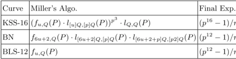
Table 3. Optimal Ate pairing formulas for target curves Curve Miller’s Algo. Final Exp. KSS-16 (fu,Q(P ) · l[u]Q,[p]Q(P ))p
3
· lQ,Q(P ) (p16− 1)/r
BN f6u+2,Q(P ) · l[6u+2]Q,[p]Q(P ) · l[6u+2+p]Q,[p2]Q(P ) (p12− 1)/r
BLS-12 fu,Q(P ) (p12− 1)/r
KSS-16 Curve: In what follows, we consider P ∈ G1 ⊂ E(Fp) and Q ∈ G2⊂
E(Fp16) for KSS-16 curves. Ate pairing e(Q, P ) is given as follows:
e(Q, P ) = ft−1,Q(P )
p16 −1
r , (6)
where ft−1,Q(P ) symbolizes the output of Miller’s algorithm and blog2(t − 1)c
is the loop length. The bilinearity of Ate pairing is satisfied after calculating the final exponentiation (pk− 1)/r.
Vercauteren proposed more efficient variant of Ate pairing named as Optimal-Ate pairing [29] where the Miller’s loop length reduced to blog2uc. The previous work of Zhang et al. [31] has derived the optimal Ate pairing on the KSS-16 curve which is defined as follows with fu,Q(P ) is the Miller function evaluated
on P :
eopt(Q, P ) = ((fu,Q(P ) · l[u]Q,[p]Q(P ))p
3
· lQ,Q(P ))
p16 −1
r . (7)
The formulas for Optimal-Ate pairing for the target curves are given in Table 3.
The naive calculation procedure of Optimal-Ate pairing is shown in Alg. 1. In what follows, the calculation steps from 1 to 11, shown in Alg.1, is identified as Miller’s Algorithm (MA) and step 12 is the final exponentiation (FE). Steps 2-7 are specially named as Miller’s loop. Steps 3, 5, 7 are the line evaluation to-gether with elliptic curve doubling (ECD) and addition (ECA) inside the Miller’s loop and steps 9, 11 are the line evaluation. These line evaluation steps are the key steps to accelerate the loop calculation. The authors extended the work of [23],[20] for KSS-16 curve to calculate pseudo 8-sparse multiplication described in Sect. 3. The ECA and ECD are also calculated efficiently in the twisted curve. The Q2← [p]Q term of step 8 is calculated by applying one skew Frobenius map
over Fp4and f1← fp 3
Fp16. Step 12, FE is calculated by applying Ghammam et al.’s work for KSS-16
curve [16].
Algorithm 1: Optimal Ate pairing on KSS-16 curve
Input: u, P ∈ G1, Q ∈ G02
Output: (Q, P ) f ← 1, T ← Q
1
for i = blog2(u)c downto 1 do
2 f ← f2· l T ,T(P ), T ← [2]T 3 if u[i] = 1 then 4 f ← f · lT ,Q(P ), T ← T + Q 5 if u[i] = −1 then 6 f ← f · lT ,−Q(P ), T ← T − Q 7 Q1← [u]Q, Q2← [p]Q 8 f ← f · lQ1,Q2(P ) 9 f1← fp 3 , f ← f · f1 10 f ← f · lQ,Q(P ) 11 f ← fp16 −1r 12 return f 13 2.4 Twist of KSS-16 Curves
In the context of Type 3 pairing, there exists a twisted curve with a group of rational points of order r, isomorphic to the group where rational point Q ∈ E(Fpk)[r] ∩ Ker(πp − [p]) belongs to. This sub-field isomorphic rational
point group includes a twisted isomorphic point of Q, typically denoted as Q0∈ E0
(Fpk/d), where k is the embedding degree and d is the twist degree.
Since points on the twisted curve are defined over a smaller field than Fpk,
therefore ECA and ECD become faster. However, when required in the Miller’s algorithm’s line evaluation, the points can be quickly mapped to points on E(Fpk). Since the pairing-friendly KSS-16 [19] curve has CM discriminant of
D = 1 and 4|k; therefore, quartic twist is available.
Quartic twist Let β be a certain quadratic non-residue in Fp4. The quartic
twisted curve E0 of KSS-16 curve E defined in Eq. (1) and their isomorphic mapping ψ4 are given as follows:
E0 : y2= x3+ axβ−1, a ∈ Fp,
ψ4: E0(Fp4)[r] 7−→ E(Fp16)[r] ∩ Ker(πp− [p]),
(x, y) 7−→ (β1/2x, β3/4y), (8)
where Ker(·) denotes the kernel of the mapping and πpdenotes Frobenius
Table 4. Vector representation of Q = (xQ, yQ) ∈ G2⊂ Fp16
1 α β αβ γ αγ βγ αβγ ω αω βω αβω γω αγω βγω αβγω
xQ 0 0 0 0 b4 b5 b6 b7 0 0 0 0 0 0 0 0
yQ 0 0 0 0 0 0 0 0 0 0 0 0 b12 b13 b14 b15
Table 4 shows the vector representation of Q = (xQ, yQ) = (β1/2xQ0, β3/4yQ0) ∈
Fp16 according to the given towering in Eq. (3). Here, xQ0 and yQ0 are the
coor-dinates of rational point Q0 on quartic twisted curve E0.
3
Proposal
3.1 Overview: Sparse and Pseudo-Sparse Multiplication
Aranha et al. [1, Section 4] and Costello et al. [10] have well optimized the Miller’s algorithm in Jacobian coordinates by 6-sparse multiplication 4 for BN curve. Mori et al. [23] have shown the pseudo 8-sparse multiplication5 for BN curve by adapting affine coordinates where the sextic twist is available. It is found that pseudo 8-sparse was efficient than 7-sparse and 6-sparse in Jacobian coordinates.
Let us consider T = (γxT0, γωyT0), Q = (γxQ0, γωyQ0) and P = (xP, yP),
where xp, yp ∈ Fp given in affine coordinates on the curve E(Fp16) such that
T0= (xT0, yT0), Q0 = (xQ0, yQ0) are in the twisted curve E0 defined over Fp4. Let
the elliptic curve doubling of T + T = R(xR, yR). The 7-sparse multiplication
for KSS-16 can be derived as follows.
lT ,T(P ) = (yp− yT0γω) − λT ,T(xP− xT0γ), when T = Q, λT ,T = 3x2 T 0γ 2+a 2yT 0γω = 3x2 T 0γω −1+a(γω)−1 2yT 0 = (3x2 T 0+ac −1αβ)ω 2yT 0 = λ 0 T ,Tω, since γω−1 = ω, (γω)−1= ωβ−1, and
aβ−1= (a + 0α + 0β + 0αβ)β−1= aβ−1= ac−1αβ, where α2= c.
Now the line evaluation and ECD are obtained as follows:
lT ,T(P ) = yp− xpλ0T ,Tω + (xT0λ0T ,T− yT0)γω, x2T0 = (λ0 T ,T) 2ω2 − 2x T0γ = ((λ0 T ,T) 2 − 2x T0)γ y2T0 = (xT0γ − x2T0γ)λ0T ,Tω − yT0γω = (xT0λ0T ,T− x2T0λ0T ,T− yT0)γω. 4 6-Sparse refers the state when in a vector (multiplier/multiplicand), among the 12
coefficients 6 of them are zero.
5 Pseudo 8-sparse refers to a certain length of vector’s coefficients where instead of 8
The above calculations can be optimized as follows: A = 2y1 T 0, B = 3x 2 T0 + ac−1, C = AB, D = 2xT0, x2T0 = C2− D, E = CxT0− yT0, y2T0= E − Cx2T0, lT ,T(P ) = yP+ Eγω − CxPω = yP + F ω + Eγω, (9) where F = −CxP.
The elliptic curve addition phase (T 6= Q) and line evaluation of lT ,Q(P ) can
also be optimized similar to the above procedure. Let the elliptic curve addition of T + Q = R(xR, yR). lT ,Q(P ) = (yp− yT0γω) − λT ,Q(xP− xT0γ), T 6= Q, λT ,Q= (yQ0−yT 0)γω (xQ0−xT 0)γ = (yQ0−yT 0)ω xQ0−xT 0 = λ 0 T ,Qω, xR= (λ0T ,Q) 2ω2 − x T0γ − xQ0γ = ((λ0T ,Q)2 − xT0 − xQ0)γ yR= (xT0γ − xRγ)λ0T ,Qω − yT0γω = (xT0λ0T ,Q− xR0λ0T ,Q− yT0)γω.
Representing the above line equations using variables as following :
A = x 1 Q0−xT 0, B = yQ 0− yT0, C = AB, D = xT0 + xQ0, xR0 = C2− D, E = CxT0− yT0, yR0 = E − CxR0, lT ,Q(P ) = yP + Eγω − CxPω = yP + F ω + Eγω, (10) F = −CxP,
Here all the variables (A, B, C, D, E, F ) are calculated as Fp4 elements. The
position of the yP, E and F in Fp16 vector representation is defined by the basis
element 1, γω and ω as shown in Table 4. Therefore, among the 16 coefficients of lT ,T(P ) and lT ,Q(P ) ∈ Fp16, only 9 coefficients yP ∈ Fp, CxP ∈ Fp4 and
E ∈ Fp4 are non-zero. The remaining 7 zero coefficients leads to an efficient
multiplication, usually called sparse multiplication. This particular instance in KSS-16 curve is named as 7-sparse multiplication.
3.2 Pseudo 8-Sparse Multiplication for BN and BLS-12 Curve
Here we have followed Mori et al.’s [23] procedure to derive pseudo 8-sparse multiplication for the parameter settings of [3] for BN and BLS-12 curves. For the new parameter settings, the towering is given as Eq. (4) for both BN and BLS-12 curve. However, the curve form E : y2= x3
+ b, b ∈ Fp is identical for
both BN and BLS-12 curve. The sextic twist obtained for these curves are also identical. Therefore, in what follows this paper will denote both of them as Eb
defined over Fp12.
Sextic twist of BN and BLS-12 curve: Let (α + 1) be a certain quadratic and cubic non-residue in Fp2. The sextic twisted curve Eb0 of curve Eband their
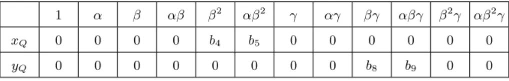
Table 5. Vector representation of Q = (xQ, yQ) ∈ G2⊂ Fp12 vector representation
1 α β αβ β2 αβ2 γ αγ βγ αβγ β2γ αβ2γ
xQ 0 0 0 0 b4 b5 0 0 0 0 0 0
yQ 0 0 0 0 0 0 0 0 b8 b9 0 0
isomorphic mapping ψ6 are given as follows:
Eb0 : y2= x3+ b(α + 1), b ∈ Fp,
ψ6: Eb0(Fp2)[r] 7−→ Eb(Fp12)[r] ∩ Ker(πp− [p]),
(x, y) 7−→ ((α + 1)−1xβ, (α + 1)−1yβ2γ). (11) The line evaluation and ECD/ECA can be obtained in affine coordinate for the rational point P and Q0, T0∈ E0
b(Fp2) as follows:
Elliptic curve addition when T0 6= Q0 and T0+ Q0= R0(x R0, yR0) A = x 1 Q0−xT 0, B = yQ 0− yT0, C = AB, D = xT0 + xQ0, xR0 = C2− D, E = CxT0− yT0, yR0 = E − CxR0, lT0,Q0(P ) = yP + (α + 1)−1Eβγ − (α + 1)−1CxPβ2γ, (12a) y−1P lT0,Q0(P ) = 1 + (α + 1)−1Ey−1 P βγ − (α + 1) −1Cx Py−1P β 2γ, (12b)
Elliptic curve doubling when T0 = Q0 A = 2y1 T 0, B = 3x 2 T0, C = AB, D = 2xT0, x2T0 = C2− D, E = CxT0− yT0, y2T0= E − Cx2T0, lT0,T0(P ) = yP+ (α + 1)−1Eβγ − (α + 1)−1CxPβ2γ, (13a) y−1P lT0,T0(P ) = 1 + (α + 1)−1EyP−1βγ − (α + 1)−1CxPyP−1β2γ, (13b)
The line evaluations of Eq. (12b) and Eq. (13b) are identical and more sparse than Eq. (12a) and Eq. (13a). Such sparse form comes with a cost of computa-tion overhead. But such overhead can be minimized by the following isomorphic mapping, which also accelerates the Miller’s loop iteration.
Isomorphic mapping of P ∈ G17→ ˆP ∈ G01: ˆ E : y2= x3+ bˆz, ˆ E(Fp)[r] 7−→ E(Fp)[r], (x, y) 7−→ (ˆz−1x, ˆz−3/2y), (14) where ˆz ∈ Fpis a quadratic and cubic residue in Fp. Eq. (14) maps rational point
P to ˆP (xPˆ, yPˆ) such that (xPˆ, yP−1ˆ ) = 1. The twist parameter ˆz is obtained as:
ˆ
z = (xPyP−1) 6
From the Eq. (15) ˆP and ˆQ0 is given as ˆ P (xPˆ, yPˆ) = (xPz−1, yPz−3/2) = (x3Py −2 P , x 3 Py −2 P ), (16a) ˆ Q0(x ˆ Q0, yQˆ0) = (x2Py−2P xQ0, x3Py−3P yQ0). (16b)
Using Eq. (16a) and Eq. (16b) the line evaluation of Eq. (13b) becomes
y−1ˆ P lTˆ0, ˆT0( ˆP ) = 1 + (α + 1)−1Ey−1ˆ P βγ − (α + 1) −1Cx ˆ Py −1 ˆ P β 2γ, ˆ lTˆ0, ˆT0( ˆP ) = 1 + (α + 1) −1Ey−1 ˆ P βγ − (α + 1) −1Cβ2γ. (17a)
The Eq. (12b) becomes similar to Eq. (17a). The calculation overhead can be reduced by pre-computation of (α + 1)−1, y−1ˆ
P and ˆP , ˆQ
0 mapping using x−1 P
and y−1P as shown by Mori et al. [23].
Finally, pseudo 8-sparse multiplication for BN and BLS-12 is given in
Algorithm 2: Pseudo 8-sparse multiplication for BN and BLS-12 curves Input: a, b ∈ Fp12 a = (a0+ a1β + a2β2) + (a3+ a4β + a5β2)γ, b = 1 + b4βγ + b5β2γ where ai, bj, ci∈ Fp2(i = 0, · · ·, 5, j = 4, 5) Output: c = ab = (c0+ c1β + c2β2) + (c3+ c4β + c5β2)γ ∈ Fp12 c4← a0× b4, t1← a1× b5, t2← a0+ a1, S0← b4+ b5 1 c5← t2× S0− (c4+ t1), t2 ← a2× b5, t2← t2× (α + 1) 2 c4← c4+ t2, t0← a2× b4, t0← t0+ t1 3 c3← t0× (α + 1), t0← a3× b4, t1← a4× b5, t2← a3+ a4 4 t2← t2× S0− (t0+ t1) 5 c0← t2× (α + 1), t2← a5× b4, t2← t1+ t2 6 c1← t2× (α + 1), t1← a5× b5, t1← t1× (α + 1) 7 c2← t0+ t1 8 c ← c + a 9 return c = (c0+ c1β + c2β2) + (c3+ c4β + c5β2)γ 10
3.3 Pseudo 8-sparse Multiplication for KSS-16 Curve
The main idea of pseudo 8-sparse multiplication is finding more sparse form of Eq. (9) and Eq. (10), which allows to reduce the number of multiplication of Fp16 vector during Miller’s algorithm evaluation. To obtains the same, yP−1
is multiplied to both side of Eq. (9) and Eq. (10), since yP remains the same
through the Miller’s algorithms loop calculation.
y−1P lT ,P(P ) = 1 − CxPyP−1ω + Ey−1P γω, (18a)
y−1P lT ,Q(P ) = 1 − CxPyP−1ω + Ey −1
P γω, (18b)
Although the Eq. (18a) and Eq. (18b) do not get more sparse, but 1st coeffi-cient becomes 1. Such vector is titled as pseudo sparse form in this paper. This
form realizes more efficient Fp16 vectors multiplication in Miller’s loop. However,
the Eq. (18b) creates more computation overhead than Eq. (10), i.e., computing yP−1lT ,Q(P ) in the left side and xPy−1P , Ey
−1
P on the right. The same goes
be-tween Eq. (18a) and Eq. (9). Since the computation of Eq. (18a) and Eq. (18b) are almost identical, therefore the rest of the paper shows the optimization tech-nique for Eq. (18a). To overcome these overhead computations, the following techniques can be applied.
– xPyP−1 is omitted by applying further isomorphic mapping of P ∈ G1.
– y−1P can be pre-computed. Therefore, the overhead calculation of EyP−1 will cost only 2 Fp multiplication.
– y−1P lT ,T(P ) doesn’t effect the pairing calculation cost since the final
expo-nentiation cancels this multiplication by yP−1∈ Fp.
To overcome the CxPyP−1 calculation cost, xPy−1P = 1 is expected. To
ob-tain xPyP−1 = 1, the following isomorphic mapping of P = (xP, yP) ∈ G1 is
introduced.
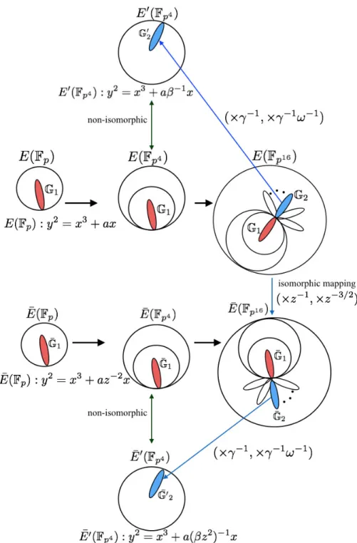
Isomorphic map of P = (xP, yP) → ¯P = (xP¯, yP¯). Although the KSS-16
curve is typically defined over Fp16 as E(Fp16), but for efficient implementation
of Optimal-Ate pairing, certain operations are carried out in a quartic twisted isomorphic curve E0 defined over Fp4 as shown in Sec. 2.4. For the same, let
us consider ¯E(Fp4) is isomorphic to E(Fp4) and certain z ∈ Fp as a quadratic
residue (QR) in Fp4. A generalized mapping between E(Fp4) and ¯E(Fp4) can be
given as follows: ¯ E : y2= x3+ az−2x, ¯ E(Fp4)[r] 7−→ E(Fp4)[r], (x, y) 7−→ (z−1x, z−3/2y), where z, z−1, z−3/2∈ Fp. (19)
The mapping considers z ∈ Fp is a quadratic residue over Fp4 which can be
shown by the fact that z(p4−1)/2= 1 as follows: z(p4−1)/2= z(p−1)(p3+p2+p+1)/2
= 1(p3+p2+p+1)/2
= 1 QR ∈ Fp4 . (20)
Therefore, z is a quadratic residue over Fp4.
Now based on P = (xP, yP) be the rational point on curve E, the considered
isomorphic mapping of Eq. (19) can find a certain isomorphic rational point ¯
P = (xP¯, yP¯) on curve ¯E as follows:
y2P = x3P + axP,
yP2z−3= x3Pz−3+ axPz−3,
where ¯P = (xP¯, yP¯) = (xPz−1, yPz−3/2) and the general form of the curve ¯E is
given as follows:
y2= x3+ az−2x. (22)
To obtain the target relation xP¯yP−1¯ = 1 from above isomorphic map and rational
point ¯P , let us find isomorphic twist parameter z as follows: xP¯yP−1¯ = 1
z−1xP(z−3/2yP)−1= 1
z1/2(xP.yP−1) = 1
z = (x−1P yP)2. (23)
Now using z = (x−1P yP)2 and Eq. (21), ¯P can be obtained as
¯
P (xP¯, yP¯) = (xPz−1, yPz−3/2) = (x3PyP−2, x 3
PyP−2), (24)
where the x and y coordinates of ¯P are equal. For the same isomorphic map we can obtain ¯Q on curve ¯E defined over Fp12 as follows:
¯
Q(xQ¯, yQ¯) = (z−1xQ0γ, z−3/2yQ0γω), (25)
where from Eq. (8), Q0(xQ0, yQ0) is obtained in quartic twisted curve E0.
At this point, to use ¯Q with ¯P in line evaluation we need to find another isomorphic map that will map ¯Q 7→ ¯Q0, where ¯Q0 is the rational point on curve
¯
E0 defined over F
p4. Such ¯Q0 and ¯E0 can be obtained from ¯Q of Eq. (25) and
curve ¯E from Eq. (22) as follows:
(z−3/2yQ0γω)2= (z−1xQ0γ)3+ az−2z−1xQ0γ,
(z−3/2yQ0)2γ2ω2= (z−1xQ0)3γ3+ az−2z−1xQ0γ,
(z−3/2yQ0)2βγ = (z−1xQ0)3βγ + az−2z−1xQ0γ,
(z−3/2yQ0)2= (z−1xQ0)3+ az−2β−1z−1xQ0.
From the above equations, ¯E0 and ¯Q0 are given as,
¯ E0: y2 ¯ Q0 = x 3 ¯ Q0+ a(z 2β)−1x ¯ Q0. (26) ¯ Q0(x¯ Q0, yQ¯0) = (z−1xQ0, z−3/2yQ0) = (xQ0x2PyP−2, yQ0x3PyP−3). (27)
Now, applying ¯P and ¯Q0, the line evaluation of Eq. (18b) becomes as follows:
y−1P¯ lT¯0, ¯Q0( ¯P ) = 1 − C(xP¯yP−1¯ )γ + Ey−1P¯ γω ¯ lT¯0, ¯Q0( ¯P ) = 1 − Cγ + E(x−3P yP2)γω, (28) where xP¯yP−1¯ = 1 and yP−1¯ = z3/2yP−1 = (x −3 P y 2
P). The Eq. (18a) becomes the
same as Eq. (28). Compared to Eq. (18b), the Eq. (28) will be faster while using in Miller’s loop in combination of the pseudo 8-sparse multiplication shown in Alg.2. However, to get the above form, we need the following pre-computations once in every Miller’s Algorithm execution.
– Computing ¯P and ¯Q0,
– (x−3P y2 P) and
– z−2 term from curve ¯E0 of Eq. (26).
The above terms can be computed from x−1P and yP−1 by utilizing Montgomery trick [22], as shown in Alg. 3. The pre-computation requires 21 multiplication, 2 squaring and 1 inversion in Fp and 2 multiplication, 3 squaring in Fp4.
Algorithm 3: Pre-calculation and mapping P 7→ ¯P and Q07→ ¯Q0
Input: P = (xP, yP) ∈ G1, Q0= (xQ0, yQ0) ∈ G02 Output: ¯Q0, ¯P , y−1 P , (z) −2 A ← (xPyP)−1 1 B ← Ax2 P 2 C ← AyP 3 D ← B2 4 xQ¯0← DxQ0 5 yQ¯0 ← BDyQ0 6 xP¯, yP¯← DxP 7 y−1P ← C3y2 P 8 z−2← D2 9 return ¯Q0 = (x¯ Q0, yQ¯0), ¯P = (xP¯, yP¯), yP−1, z−2 10
The overall mapping and the curve obtained in the twisting process is shown in the Fig. 1.
Finally the Alg.4 shows the derived pseudo 8-sparse multiplication.
Algorithm 4: Pseudo 8-sparse multiplication for KSS-16 curve Input: a, b ∈ Fp16 a = (a0+ a1γ) + (a2+ a3γ)ω, b = 1 + (b2+ b3γ)ω a = (a0+ a1ω + a2ω2+ a3ω3), b = 1 + b2ω + b3ω3 Output: c = ab = (c0+ c1γ) + (c3+ c4γ)ω ∈ Fp16 t0← a3× b3× β, t1← a2× b2, t4← b2+ b3, c0← (a2+ a3) × t4− t1− t0 1 c1← t1+ t0× β 2 t2← a1× b3, t3← a0× b2, c2 ← t3+ t2× β 3 t4← (b2+ b3), c3← (a0+ a1) × t4− t3− t2 4 c ← c + a 5 return c = (c0+ c1γ) + (c3+ c4γ)ω 6 3.4 Final Exponentiation
Scott et al. [27] show the process of efficient final exponentiation (FE) fpk−1/r
by decomposing the exponent using cyclotomic polynomial Φk as
The 1st two terms of the right part are denoted as easy part since it can be easily calculated by Frobenius mapping and one inversion in affine coordinates. The last term is called hard part which mostly affects the computation performance. According to Eq. (29), the exponent decomposition of the target curves is shown in Table 6.
Table 6. Exponents of final exponentiation in pairing Curve Final exponent Easy part Hard part KSS-16 p16r−1 p8− 1 p8+1 r BN, BLS-12 p12−1 r (p 6− 1)(p2+ 1) p4−p2+1 r
This paper carefully concentrates on Miller’s algorithm for comparison and making pairing efficient. However, to verify the correctness of the bilinearity property, the authors made a “not state-of-art” implementation of Fuentes et al.’s work [14] for BN curve case and Ghammam’s et al.’s works [16,17] for KSS-16 and BLS-12 curves. For scalar multiplication by prime p, i.e., p[Q] or [p2]Q, skew Frobenius map technique by Sakemi et al. [26] is adapted.
4
Experimental Result Evaluation
This section gives details of the experimental implementation. The source code can be found in Github6. The code is not an optimal code, and the sole
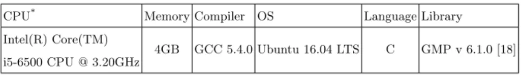
pur-pose of it compare the Miller’s algorithm among the curve families and validate the estimation of [3]. Table 7 shows implementation environment. Parameters
Table 7. Computational Environment
CPU* Memory Compiler OS Language Library
Intel(R) Core(TM) i5-6500 CPU @ 3.20GHz
4GB GCC 5.4.0 Ubuntu 16.04 LTS C GMP v 6.1.0 [18]
*Only single core is used from two cores.
chosen from [3] is shown in Table 8. Table 9 shows execution time for Miller’s algorithm implementation in millisecond for a single Optimal-Ate pairing. Re-sults here are the average of 10 pairing operation. From the result, we find that Miller’s algorithm took the least time for KSS-16. And the time is almost closer to BLS-12. The Miller’s algorithm is about 1.7 times faster in KSS-16 than BN
6
Table 8. Selected parameters for 128-bit security level [3]
Curve u HW(u) blog2uc blog2p(u)c blog2r(u)c blog2p kc
KSS-16 u = 235− 232− 218
+ 28+ 1 5 35 339 263 5424 BN u = 2114+ 2101− 214− 1 4 115 462 462 5535
BLS-12 u = −277+ 250+ 233 3 77 461 308 5532
Table 9. Comparative results of Miller’s Algorithm in [ms]. KSS-16 BN BLS-12
Miller’s Algorithm 4.41 7.53 4.91
curve. Table 12 shows that the complexity of this implementation concerning the number of Fp multiplication and squaring and the estimation of [3] are
al-most coherent for Miller’s algorithm. Table 12 also show that our derived pseudo 8-sparse multiplication for KSS-16 takes fewer Fp multiplication than Zhang et
al.’s estimation [31]. The execution time of Miller’s algorithm also goes with this estimation [3], that means KSS-16 and BLS-12 are more efficient than BN curve. Table 10 shows the complexity of Miller’s algorithm for the target curves inFp
operations count.
The operation counted in Table 10 are based on the counter in implementa-tion code. For the implementaimplementa-tion of big integer arithmetic mpz t data type of GMP [18] library has been used. For example, multiplication between 2 mpz t variables are counted as Fpmultiplication and multiplication between one mpz t
and one “unsigned long” integer can also be treated as Fp multiplication.
Ba-sis multiplication refers to the vector multiplication such as (ao+ a1α)α where
a0, a1∈ Fp and α is the basis element in Fp2.
Table 10. Complexity of this implementation in Fpfor Miller’s algorithm [single
pair-ing operation]
Multiplication
Squaring Addition/ Subtraction
Basis Multiplication Inversion mpz t * mpz t mpz t * ui
KSS-16 6162 144 903 23956 3174 43
BN 10725 232 157 35424 3132 125
As said before, this work is focused on Miller’s algorithm. However, the au-thors made a “not state-of-art” implementation of some final exponentiation algorithms [16,14,17]. Table 11 shows the total final exponentiation time in [ms]. Here final exponentiation of KSS-16 is slower than BN and BLS-12. We have applied square and multiply technique for exponentiation by integer u in the hard part since the integer u given in the sparse form. However, Barbulescu et al. [3] mentioned that availability of compressed squaring [1] for KSS-16 will lead a fair comparison using final exponentiation.
Table 11. Final exponentiation time (not state-of-art) in [ms] KSS-16 BN BLS-12 Final exponentiation 17.32 11.65 12.03
Table 12. Complexity comparison of Miller’s algorithm between this implementation and Barbulescu et al.’s [3] estimation [Multiplication + Squaring in Fp]
KSS-16 BN BLS-12 Barbulescu et al. [3] 7534Mp 12068Mp 7708Mp
This implementation 7209Mp 11114Mp 7202Mp
5
Conclusion and Future Work
This paper has presented two major ideas.
– Finding efficient Miller’s algorithm implementation technique for Optimal-Ate pairing for the less studied KSS-16 curve. The author’s presented pseudo 8-sparse multiplication technique for KSS-16. They also extended such mul-tiplication for BN and BLS-12 according to [23] for the new parameter. – Verifying Barbulescu and Duquesne’s conclusion [3] for calculating
Optimal-Ate pairing at 128-bit security level; that is, BLS-12 and less studied KSS-16 curves are more efficient choices than well studied BN curves for new parameters. This paper finds that Barbulescu and Duquesne’s conclusion on BLS-12 is correct as it takes the less time for Miller’s algorithm. Applying the derived pseudo 8-sparse multiplication, Miller’s algorithm in KSS-16 is also more efficient than BN.
As a prospective work authors would like to evaluate the performance by finding compressed squaring for KSS-16’s final exponentiation along with scalar multi-plication of G1, G2and exponentiation of GT. The execution time for the target
environment can be improved by a careful implementation using assembly lan-guage for prime field arithmetic.
Acknowledgment
This work was partially supported by the Strategic Information and Commu-nications R&D Promotion Programme (SCOPE) of Ministry of Internal Af-fairs and Communications, Japan and The French projects ANR-16-CE39-0012 “SafeTLS” and ANR-11-LABX-0020-01 “Centre Henri Lebesgue”.
References
1. Aranha, D.F., Karabina, K., Longa, P., Gebotys, C.H., L´opez, J.: Faster explicit formulas for computing pairings over ordinary curves. In: Eurocrypt. vol. 6632, pp. 48–68. Springer (2011)
2. Bailey, D.V., Paar, C.: Efficient arithmetic in finite field extensions with application in elliptic curve cryptography. Journal of cryptology 14(3), 153–176 (2001) 3. Barbulescu, R., Duquesne, S.: Updating key size estimations for pairings.
Cryptol-ogy ePrint Archive, Report 2017/334 (2017), http://eprint.iacr.org/2017/334 4. Barreto, P.S., Lynn, B., Scott, M.: Constructing elliptic curves with prescribed em-bedding degrees. In: Security in Communication Networks, pp. 257–267. Springer (2002)
5. Barreto, P.S., Naehrig, M.: Pairing-friendly elliptic curves of prime order. In: In-ternational Workshop on Selected Areas in Cryptography, SAC 2005. pp. 319–331. Springer (2005)
6. Benger, N., Scott, M.: Constructing tower extensions of finite fields for implemen-tation of pairing-based cryptography. In: Arithmetic of finite fields, pp. 180–195. Springer (2010)
7. Boneh, D., Boyen, X., Shacham, H.: Short group signatures. In: Advances in Cryptology–CRYPTO 2004. pp. 41–55. Springer (2004)
8. Boneh, D., Lynn, B., Shacham, H.: Short signatures from the weil pairing. In: Advances in CryptologyASIACRYPT 2001, pp. 514–532. Springer (2001)
9. Cohen, H., Frey, G., Avanzi, R., Doche, C., Lange, T., Nguyen, K., Vercauteren, F.: Handbook of elliptic and hyperelliptic curve cryptography. CRC press (2005) 10. Costello, C., Lange, T., Naehrig, M.: Faster pairing computations on curves with
high-degree twists. In: International Workshop on Public Key Cryptography. pp. 224–242. Springer (2010)
11. Devegili, A.J., O’hEigeartaigh, C., Scott, M., Dahab, R.: Multiplication and squar-ing on pairsquar-ing-friendly fields. IACR Cryptology ePrint Archive 2006, 471 (2006) 12. Duquesne, S., Mrabet, N.E., Haloui, S., Rondepierre, F.: Choosing and generating
parameters for low level pairing implementation on bn curves. Cryptology ePrint Archive, Report 2015/1212 (2015), http://eprint.iacr.org/2015/1212
13. Freeman, D., Scott, M., Teske, E.: A taxonomy of pairing-friendly elliptic curves. Journal of cryptology 23(2), 224–280 (2010)
14. Fuentes-Casta˜neda, L., Knapp, E., Rodr´ıguez-Henr´ıquez, F.: Faster hashing to ${\mathbb G} 2$. In: Selected Areas in Cryptography - 18th International Work-shop, SAC 2011, Toronto, ON, Canada, August 11-12, 2011, Revised Selected Pa-pers. pp. 412–430 (2011), https://doi.org/10.1007/978-3-642-28496-0_25
15. Galbraith, S.D., Paterson, K.G., Smart, N.P.: Pairings for cryptographers. Discrete Applied Mathematics 156(16), 3113–3121 (2008)
16. Ghammam, L., Fouotsa, E.: Adequate elliptic curves for computing the product of n pairings. In: International Workshop on the Arithmetic of Finite Fields. pp. 36–53. Springer (2016)
17. Ghammam, L., Fouotsa, E.: On the computation of the optimal ate pairing at the 192-bit security level. Cryptology ePrint Archive, Report 2016/130 (2016), http://eprint.iacr.org/2016/130
18. Granlund, T., the GMP development team: GNU MP: The GNU Multiple Precision Arithmetic Library, 6.1.0 edn. (2015), http://gmplib.org
19. Kachisa, E., Schaefer, E., Scott, M.: Constructing brezing-weng pairing-friendly elliptic curves using elements in the cyclotomic field. Pairing-Based Cryptography– Pairing 2008 pp. 126–135 (2008)
20. Khandaker, M.A.A., Ono, H., Nogami, Y., Shirase, M., Duquesne, S.: An improve-ment of optimal ate pairing on KSS curve with pseudo 12-sparse multiplication. In: International Conference on Information Security and Cryptology. pp. 208–219. Springer (2016)
21. Kim, T., Barbulescu, R.: Extended tower number field sieve: A new complexity for the medium prime case. In: Advances in Cryptology - CRYPTO 2016 - Proceedings, Part I. pp. 543–571. Springer (2016)
22. Montgomery, P.L.: Speeding the pollard and elliptic curve methods of factorization. Mathematics of computation 48(177), 243–264 (1987)
23. Mori, Y., Akagi, S., Nogami, Y., Shirase, M.: Pseudo 8–sparse multiplica-tion for efficient ate–based pairing on barreto–naehrig curve. In: Pairing-Based Cryptography–Pairing 2013, pp. 186–198. Springer (2013)
24. Okamoto, T., Takashima, K.: Fully secure functional encryption with general re-lations from the decisional linear assumption. In: Annual Cryptology Conference. pp. 191–208. Springer (2010)
25. Sakai, R.: Cryptosystems based on pairing. In: The 2000 Symposium on Cryptog-raphy and Information Security, Okinawa, Japan, Jan. pp. 26–28 (2000)
26. Sakemi, Y., Nogami, Y., Okeya, K., Kato, H., Morikawa, Y.: Skew frobenius map and efficient scalar multiplication for pairing–based cryptography. In: International Conference on Cryptology and Network Security. pp. 226–239. Springer (2008) 27. Scott, M., Benger, N., Charlemagne, M., Perez, L.J.D., Kachisa, E.J.: On the final
exponentiation for calculating pairings on ordinary elliptic curves. In: Pairing-Based Cryptography - Pairing 2009, Third International Conference, Palo Alto, CA, USA, August 12-14, 2009, Proceedings. pp. 78–88 (2009), https://doi.org/ 10.1007/978-3-642-03298-1_6
28. Silverman, J.H., Cornell, G., Artin, M.: Arithmetic geometry. Springer (1986) 29. Vercauteren, F.: Optimal pairings. Information Theory, IEEE Transactions on
56(1), 455–461 (2010)
30. Weil, A., et al.: Numbers of solutions of equations in finite fields. Bull. Amer. Math. Soc 55(5), 497–508 (1949)
31. Zhang, X., Lin, D.: Analysis of optimum pairing products at high security levels. In: Progress in Cryptology - INDOCRYPT 2012. pp. 412–430. Springer (2012)

![Table 8. Selected parameters for 128-bit security level [3]](https://thumb-eu.123doks.com/thumbv2/123doknet/14371455.504433/18.892.204.719.239.342/table-selected-parameters-bit-security-level.webp)
