HAL Id: hal-00973509
https://hal.archives-ouvertes.fr/hal-00973509v2
Submitted on 19 Dec 2014
HAL is a multi-disciplinary open access
archive for the deposit and dissemination of sci-entific research documents, whether they are pub-lished or not. The documents may come from teaching and research institutions in France or abroad, or from public or private research centers.
L’archive ouverte pluridisciplinaire HAL, est destinée au dépôt et à la diffusion de documents scientifiques de niveau recherche, publiés ou non, émanant des établissements d’enseignement et de recherche français ou étrangers, des laboratoires publics ou privés.
Distributed under a Creative Commons Attribution - NonCommercial - NoDerivatives| 4.0
Exponential convergence to quasi-stationary distribution
and Q-process
Nicolas Champagnat, Denis Villemonais
To cite this version:
Nicolas Champagnat, Denis Villemonais. Exponential convergence to quasi-stationary distribution and Q-process. Probability Theory and Related Fields, Springer Verlag, 2016, 164 (1), pp.243-283. �10.1007/s00440-014-0611-7�. �hal-00973509v2�
Exponential convergence to quasi-stationary
distribution and Q-process
Nicolas Champagnat1,2, Denis Villemonais1,2
December 23, 2014
Abstract
For general, almost surely absorbed Markov processes, we obtain necessary and sufficient conditions for exponential convergence to a unique quasi-stationary distribution in the total variation norm. These conditions also ensure the existence and exponential ergodicity of the Q-process (the process conditioned to never be absorbed). We ap-ply these results to one-dimensional birth and death processes with catastrophes, multi-dimensional birth and death processes, infinite-dimensional population models with Brownian mutations and neutron transport dynamics absorbed at the boundary of a bounded domain.
Keywords: process with absorption; quasi-stationary distribution; Q-process; Dobrushin’s ergodicity coefficient; uniform mixing property; birth and death process; neutron transport process.
2010 Mathematics Subject Classification. Primary: 60J25; 37A25; 60B10; 60F99. Secondary: 60J80; 60G10; 92D25.
1
Introduction
Let (Ω, (Ft)t≥0, (Xt)t≥0, (Pt)t≥0, (Px)x∈E∪{∂}) be a time homogeneous Markov
process with state space E ∪ {∂} [31, Definition III.1.1], where (E, E) is a measurable space and ∂ 6∈ E. We recall that Px(X0 = x) = 1, Ptis the
tran-sition function of the process satisfying the usual measurability assumptions and Chapman-Kolmogorov equation. The family (Pt)t≥0 defines a
semi-group of operators on the set B(E ∪ {∂}) of bounded Borel functions on
1
Universit´e de Lorraine, IECN, Campus Scientifique, B.P. 70239, Vandœuvre-l`es-Nancy Cedex, F-54506, France
2
Inria, TOSCA team, Villers-l`es-Nancy, F-54600, France.
E ∪ ∂ endowed with the uniform norm. We will also denote by p(x; t, dy) its transition kernel, i.e. Ptf (x) =RE∪{∂}f (y)p(x; t, dy) for all f ∈ B(E ∪ {∂}).
For all probability measure µ on E ∪ {∂}, we will use the notation Pµ(·) :=
Z
E∪{∂}
Px(·)µ(dx).
We shall denote by Ex (resp. Eµ) the expectation corresponding to Px (resp.
Pµ).
We consider a Markov processes absorbed at ∂. More precisely, we as-sume that Xs= ∂ implies Xt= ∂ for all t ≥ s. This implies that
τ∂ := inf{t ≥ 0, Xt= ∂}
is a stopping time. We also assume that τ∂ < ∞ Px-a.s. for all x ∈ E and
for all t ≥ 0 and ∀x ∈ E, Px(t < τ∂) > 0.
Our first goal is to prove that Assumption (A) below is a necessary and sufficient criterion for the existence of a unique quasi-limiting distribution α on E for the process (Xt, t ≥ 0), i.e. a probability measure α such that
for all probability measure µ on E and all A ∈ E, lim
t→+∞Pµ(Xt∈ A | t < τ∂) = α(A), (1.1)
where, in addition, the convergence is exponential and uniform with respect to µ and A. In particular, α is also the unique quasi-stationary distribu-tion [28], i.e. the unique probability measure α such that Pα(Xt ∈ · | t <
τ∂) = α(·) for all t ≥ 0.
Assumption (A) There exists a probability measure ν on E such that (A1) there exists t0, c1 > 0 such that for all x ∈ E,
Px(Xt0 ∈ · | t0 < τ∂) ≥ c1ν(·);
(A2) there exists c2> 0 such that for all x ∈ E and t ≥ 0,
Pν(t < τ∂) ≥ c2Px(t < τ∂).
Theorem 1.1. Assumption (A) implies the existence of a probability mea-sure α on E such that, for any initial distribution µ,
kPµ(Xt∈ · | t < τ∂) − α(·)kT V ≤ 2(1 − c1c2)⌊t/t0⌋, (1.2)
where ⌊·⌋ is the integer part function and k · kT V is the total variation norm.
Conversely, if there is uniform exponential convergence for the total vari-ation norm in (1.1), then Assumption (A) holds true.
Stronger versions of this theorem and of the other results presented in the introduction will be given in the next sections.
The quasi-stationary distribution describes the distribution of the pro-cess on the event of non-absorption. It is well known (see [28]) that when α is a quasi-stationary distribution, there exists λ0 > 0 such that, for all
t ≥ 0,
Pα(t < τ∂) = e−λ0t. (1.3)
The following proposition characterizes the limiting behaviour of the ab-sorption probability for other initial distributions.
Proposition 1.2. There exists a non-negative function η on E ∪ {∂}, pos-itive on E and vanishing on ∂, such that
µ(η) = lim
t→∞e λ0tP
µ(t < τ∂),
where the convergence is uniform on the set of probability measures µ on E. Our second goal is to study consequences of Assumption (A) on the behavior of the process X conditioned to never be absorbed, usually referred to as the Q-process (see [1] in discrete time and for example [5] in continuous time).
Theorem 1.3. Assumption (A) implies that the family (Qx)x∈E of
proba-bility measures on Ω defined by Qx(A) = lim
t→+∞Px(A | t < τ∂), ∀A ∈ Fs, ∀s ≥ 0,
is well defined and the process (Ω, (Ft)t≥0, (Xt)t≥0, (Qx)x∈E) is an E-valued
homogeneous Markov process. In addition, this process admits the unique invariant distribution
β(dx) = Rη(x)α(dx)
Eη(y)α(dy)
and, for any x ∈ E,
kQx(Xt∈ ·) − βkT V ≤ 2(1 − c1c2)⌊t/t0⌋.
The study of quasi-stationary distributions goes back to [38] for branch-ing processes and [12, 33, 13] for Markov chains in finite or denumerable state spaces, satisfying irreducibility assumptions. In these works, the exis-tence and the convergence to a quasi-stationary distribution are proved using
spectral properties of the generator of the absorbed Markov process. This is also the case for most further works. For example, a extensively developed tool to study birth and death processes is based on orthogonal polynomials techniques of [23], applied to quasi-stationary distributions in [22, 6, 34]. For diffusion processes, we can refer to [30] and more recently [4, 5, 26], all based on the spectral decomposition of the generator. Most of these works only study one-dimensional processes, whose reversibility helps for the spectral decomposition. Processes in higher dimensions were studied either assuming self-adjoint generator in [5], or using abstract criteria from spectral theory like in [30, 10] (the second one in infinite dimension). Other formulations in terms of abstract spectral theoretical criteria were also studied in [24]. The reader can refer to [28, 11, 36] for introductory presentations of the topic.
Most of the previously cited works do not provide convergence results nor estimates on the speed of convergence. The articles studying these questions either assume abstract conditions which are very difficult to check in practice [33, 24], or prove exponential convergence for very weak norms [4, 5, 26].
More probabilistic methods were also developed. The older reference is based on a renewal technique [21] and proves the existence and convergence to a quasi-stationary distribution for discrete processes for which Assump-tion (A1) is not satisfied. More recently, one-dimensional birth and death processes with a unique quasi-stationary distribution have been shown to satisfy (1.1) with uniform convergence in total variation [27]. Convergence in total variation for processes in discrete state space satisfying strong mix-ing conditions was obtained in [9] usmix-ing Flemmix-ing-Viot particle systems whose empirical distribution approximates conditional distributions [37]. Sufficient conditions for exponential convergence of conditioned systems in discrete time can be found in [15] with applications of discrete generation particle techniques in signal processing, statistical machine learning, and quantum physics. We also refer the reader to [16, 17, 18] for approximations tech-niques of non absorbed trajectories in terms of genealogical trees.
In this work, we obtain in Section 2 necessary and sufficient conditions for exponential convergence to a unique quasi-stationary distribution for general (virtually any) Markov processes (we state a stronger form of The-orem 1.1). We also obtain spectral properties of the infinitesimal generator as a corollary of our main result. Our non-spectral approach and results fundamentally differ from all the previously cited references, except [27, 9] which only focus on very specific cases. In Section 3, we show, using penal-isation techniques [32], that the same conditions are sufficient to prove the existence of the Q-process and its exponential ergodicity, uniformly in total
variation. This is the first general result showing the link between quasi-stationary distributions and Q-processes, since we actually prove that, for general Markov processes, the uniform exponential convergence to a quasi-stationary distribution implies the existence and ergodicity of the Q-process. Section 4 is devoted to applications of the previous results to specific ex-amples of processes. Our goal is not to obtain the most general criteria, but to show how Assumption (A) can be checked in different practical situations. We first obtain necessary and sufficient conditions for one-dimensional birth and death processes with catastrophe in Section 4.1.1. We show next how the method of the proof can be extended to treat several multi-dimensional examples in Section 4.1.2. One of these examples is infinite-dimensional (as in [10]) and assumes Brownian mutations in a continuous type space. Our last example is the neutron transport process in a bounded domain, absorbed at the boundary (Section 4.2). This example belongs to the class of piecewise-deterministic Markov processes, for which up to our knowledge no results on quasi-stationary distributions are known. In this case, the absorption rate is unbounded, in the sense that the absorption time can-not be stochastically dominated by an exponential random variable with constant parameter. Other examples of Markov processes with unbounded absorption rate can be studied thanks to Theorem 2.1. For example, the study of diffusion processes on R+ absorbed at 0, or on Rd
+, absorbed at 0
or Rd+\ (R∗
+)d is relevant for population dynamics (see for example [4, 5])
and is studied in [8]. More generally, the great diversity of applications of the very similar probabilistic criterion for processes without absorption (see all the works building on [29]) indicates the wide range of applications and extensions of our criteria that can be expected.
The paper ends with the proof of the main results of Section 2 and 3 in Sections 5 and 6.
2
Existence and uniqueness of a quasi-stationary
distribution
2.1 Assumptions
We begin with some comments on Assumption (A).
When E is a Polish space, Assumption (A1) implies that Xtcomes back
fast in compact sets from any initial conditions. Indeed, there exists a compact set K of E such that ν(K) > 0 and therefore, infx∈EPx(τK∪{∂} <
E = (0, +∞) or N and ∂ = 0, this is implied by the fact that the process X comes down from infinity [4] (see Section 4.1 for the discrete case).
Assumption (A2) means that the highest non-absorption probability among all initial points in E has the same order of magnitude as the non-absorption probability starting from distribution ν. Note also that (A2) holds true when, for some A ∈ E such that ν(A) > 0 and some c′
2 > 0, inf y∈APy(t < τ∂) ≥ c ′ 2sup x∈E Px(t < τ∂) .
We now introduce the apparently weaker assumption (A’) and the stronger assumption (A”), proved to be equivalent in Theorem 2.1 below.
Assumption (A’) There exists a family of probability measures (νx1,x2)x1,x2∈E
on E such that,
(A1′) there exists t0, c1 > 0 such that, for all x1, x2 ∈ E,
Pxi(Xt0 ∈ · | t0< τ∂) ≥ c1νx1,x2(·) for i = 1, 2;
(A2′) there exist a constant c
2 > 0 such that for all x1, x2∈ E and t ≥ 0,
Pνx1,x2(t < τ∂) ≥ c2sup x∈E
Px(t < τ∂).
Assumption (A”) Assumption (A1) is satisfied and (A2′′) for any probability measure µ on E, the constant c
2(µ) defined by
c2(µ) := inf t≥0, ρ∈M1(E)
Pµ(t < τ∂)
Pρ(t < τ∂)
is positive, where M1(E) is the set of probability measures on E.
2.2 Results
The next result is a detailed version of Theorem 1.1.
Theorem 2.1. The following conditions (i)–(vi) are equivalent. (i) Assumption (A).
(ii) Assumption (A’). (iii) Assumption (A”).
(iv) There exist a probability measure α on E and two constants C, γ > 0 such that, for all initial distribution µ on E,
kPµ(Xt∈ · | t < τ∂) − α(·)kT V ≤ Ce−γt, ∀t ≥ 0. (2.1)
(v) There exist a probability measure α on E and two constants C, γ > 0 such that, for all x ∈ E,
kPx(Xt∈ · | t < τ∂) − α(·)kT V ≤ Ce−γt, ∀t ≥ 0.
(vi) There exists a probability measure α on E such that
Z ∞
0 x∈Esup
kPx(Xt∈ · | t < τ∂) − α(·)kT V dt < ∞. (2.2)
In this case, α is the unique quasi-stationary distribution for the process. In addition, if Assumption (A’) is satisfied, then (iv) holds with the explicit bound
kPµ(Xt∈ · | t < τ∂) − α(·)kT V ≤ 2(1 − c1c2)⌊t/t0⌋. (2.3)
This result and the others of this section are proved in Section 5.
One can expect that the constant C in (iv) might depend on µ pro-portionally to kµ − αkT V. This is indeed the case, but with a constant of
proportionality depending on c2(µ), defined in Assumption (A2”), as shown
by the following result.
Corollary 2.2. Hypotheses (i–vi) imply that, for all probability measures µ1, µ2 on E, and for all t > 0,
kPµ1(Xt∈ · | t < τ∂) − Pµ2(Xt∈ · | t < τ∂)kT V ≤
(1 − c1c2)⌊t/t0⌋
c2(µ1) ∧ c2(µ2)
kµ1− µ2kT V.
Remark 1. It immediately follows from (1.3) and (A”) that e−λ0t≤ sup ρ∈M1(E) Pρ(t < τ∂) ≤ e−λ0t c2(α) . (2.4)
In the proof of Theorem 2.1, we actually prove that one can take c2(α) = sup s>0exp Ç −λ0s − Ce (λ0−γ)s 1 − e−γs å , (2.5)
Remark 2. In the case of Markov processes without absorption, Meyn and Tweedie [29, Chapter 16] give several equivalent criteria for the exponential ergodicity with respect to k · kT V, among which are unconditioned versions
of (iv) and (v). The last results can be interpreted as an extension of these criteria to conditioned processes. Several differences remain.
1. In the case without absorption, the equivalence between the uncon-ditioned versions of criteria (iv) and (v) is obvious. In our case, the proof is not immediate.
2. In the case without absorption, the unconditioned version of criterion (vi) can be replaced by the weaker assumption supx∈EkPx(Xt ∈ ·) −
αkT V → 0 when t → +∞. Whether (vi) can be improved in such
a way remains an open problem in general. However, if one assumes that there exists c′2 > 0 such that for all t ≥ 0,
inf
ρ∈M1(E)
Pρ(t < τ∂) ≥ c′2 sup ρ∈M1(E)
Pρ(t < τ∂),
then one can adapt the arguments of Corollary 2.2 to prove that sup
x∈E
kPx(Xt∈ · | t < τ∂) − α(·)kT V −−−→ t→∞ 0
implies (i–vi).
3. The extension to quasi-stationary distributions of criteria based on Lyapunov functions as in [29] requires a different approach because the survival probability and conditional expectations can not be expressed easily in terms of the infinitesimal generator.
4. In the irreducible case, there is a weaker alternative to the Dobrushin-type criterion of Hypothesis (A1) known as Doeblin’s condition: there exist µ ∈ M1(E), ε < 1, t0, δ > 0 such that, for all measurable set A
satisfying µ(A) > ε,
inf
x∈EPx(Xt0 ∈ A) ≥ δ.
It is possible to check that the conditional version of this criterion implies the existence of a probability measure ν 6= µ such that (A1) is satisfied. Unfortunately ν is far from being explicit in this case and (A2), which must involve the measure ν, is no more a tractable condition, unless one can prove directly (A2”) instead of (A2).
It is well known (see [28]) that when α is a quasi-stationary distribution, there exists λ0 > 0 such that, for all t ≥ 0,
Pα(t < τ∂) = e−λ0t and eλ0tαPt= α. (2.6)
The next result is a detailed version of Proposition 1.2.
Proposition 2.3. There exists a non-negative function η on E ∪ {∂}, pos-itive on E and vanishing on ∂, defined by
η(x) = lim t→∞ Px(t < τ∂) Pα(t < τ∂) = lim t→+∞e λ0tP x(t < τ∂),
where the convergence holds for the uniform norm on E ∪ {∂} and α(η) = 1. Moreover, the function η is bounded, belongs to the domain of the infinites-imal generator L of the semi-group (Pt)t≥0 on (B(E ∪ {∂}), k · k∞) and
Lη = −λ0η.
In the irreducible case, exponential ergodicity is known to be related to a spectral gap property (see for instance [25]). Our results imply a similar property under the assumptions (i–vi) for the infinitesimal generator L of the semi-group on (B(E ∪ {∂}), k · k∞).
Corollary 2.4. If f ∈ B(E ∪ {∂}) is a right eigenfunction for L for an eigenvalue λ, then either
1. λ = 0 and f is constant, 2. or λ = −λ0 and f = α(f )η,
3. or λ ≤ −λ0− γ, α(f ) = 0 and f (∂) = 0.
3
Existence and exponential ergodicity of the
Q-process
We now study the behavior of the Q-process. The next result is a detailed version of Theorem 1.3.
Theorem 3.1. Assumption (A) implies the three following properties. (i) Existence of the Q-process. There exists a family (Qx)x∈E of probability
measures on Ω defined by lim
for all Fs-measurable set A. The process (Ω, (Ft)t≥0, (Xt)t≥0, (Qx)x∈E)
is an E-valued homogeneous Markov process. In addition, if X is a strong Markov process under P, then so is X under Q.
(ii) Transition kernel. The transition kernel of the Markov process X under (Qx)x∈E is given by
˜
p(x; t, dy) = eλ0tη(y)
η(x)p(x; t, dy). In other words, for all ϕ ∈ B(E) and t ≥ 0,
˜
Ptϕ(x) =
eλ0t
η(x)Pt(ηϕ)(x) (3.1)
where ( ˜Pt)t≥0 is the semi-group of X under Q.
(iii) Exponential ergodicity. The probability measure β on E defined by β(dx) = η(x)α(dx).
is the unique invariant distribution of X under Q. Moreover, for any initial distributions µ1, µ2 on E,
kQµ1(Xt∈ ·) − Qµ2(Xt∈ ·)kT V ≤ (1 − c1c2)
⌊t/t0⌋kµ
1− µ2kT V,
where Qµ=REQxµ(dx).
Note that, as an immediate consequence of Theorem 2.1, the uniform expo-nential convergence to a quasi-stationary distribution implies points (i–iii) of Theorem 3.1.
We investigate now the characterization of the Q-process in term of its weak infinitesimal generator (see [19, Ch I.6]). Let us recall the definition of the bounded pointwise convergence: for all fn, f in B(E ∪ {∂}), we say
that
b.p.- lim
n→∞fn= f
if and only if supnkfnk∞< ∞ and for all x ∈ E ∪ {∂}, fn(x) → f (x).
The weak infinitesimal generator Lw of (Pt) is defined as
Lwf = b.p.- lim
h→0
Phf − f
for all f ∈ B(E ∪ {∂}) such that the above b.p.–limit exists and b.p.- lim
h→0PhL
wf = Lwf.
We call weak domain and denote by D(Lw) the set of such functions f . We define similarly the b.p.–limit in B(E) and the weak infinitesimal generator
˜
Lw of ( ˜Pt) and its weak domain D( ˜Lw).
Theorem 3.2. Assume that (A) is satisfied. Then D( ˜Lw) = ® f ∈ B(E), ηf ∈ D(Lw) and L w(ηf ) η is bounded ´ (3.2) and, for all f ∈ D( ˜Lw),
˜
Lwf = λ0f +
Lw(ηf )
η .
If in addition E is a topological space and E is the Borel σ-field, and if for all open set U ⊂ E and x ∈ U ,
lim
h→0p(x; h, U ) = limh→0Ph1U(x) = 1, (3.3)
then the semi-group ( ˜Pt) is uniquely determined by its weak infinitesimal
generator ˜Lw.
Let us emphasize that (3.3) is obviously satisfied if the process X is almost surely c`adl`ag.
Remark 3. One can wonder if the weak infinitesimal generator can be re-placed in the previous result by the standard one. Then Hille-Yoshida The-orem would give necessary and sufficient condition for a strongly continuous contraction semi-group on a Banach space B to be characterized by its stan-dard infinitesimal generator (see for example [20, Thm 1.2.6, Prop 1.2.9]). However this is an open question that we couldn’t solve. To understand the difficulty, observe that even the strong continuity of ˜P cannot be easily deduced from the strong continuity of P : in view of (3.1), if ηf ∈ B, we have P˜tf − f ∞−−→ t→0 0 ⇔ 1 η(Pt(ηf ) − ηf ) ∞ −−→ t→0 0.
We don’t know whether the last convergence can be deduced from the strong continuity of P or if counter examples exist.
4
Applications
This section is devoted to the application of Theorems 2.1 and 3.1 to discrete and continuous examples. Our goal is to show how Assumption (A) can be checked in different practical situations.
4.1 Generalized birth and death processes
Our goal is to apply our results to generalized birth and death processes. In subsection 4.1.1, we extend known criteria to one dimensional birth and death processes with catastrophe. In subsection 4.1.2, we apply a similar method to multi-dimensional and infinite dimensional birth and death pro-cesses.
4.1.1 Birth and death processes with catastrophe
We consider an extension of classical birth and death processes with pos-sible mass extinction. Our goal is to extend the recent result from [27] on the characterisation of exponential convergence to a unique quasi-stationary distribution. The existence of quasi-stationary distributions for similar pro-cesses was studied in [35].
Let X be a birth and death process on Z+ with birth rates (bn)n≥0 and
death rates (dn)n≥0 with b0 = d0 = 0 and bk, dk > 0 for all k ≥ 1. We also
allow the process to jump to 0 from any state n ≥ 1 at rate an ≥ 0. In
particular, the jump rate from 1 to 0 is a1+ d1. This process is absorbed in
∂ = 0.
Theorem 4.1. Assume that supn≥1an < ∞. Conditions (i-vi) of
Theo-rem 2.1 are equivalent to
S :=X k≥1 1 dkαk X l≥k αl < ∞, (4.1) with αk= Ä Qk−1 i=1 bi ä /ÄQk i=1di ä .
Moreover, there exist constants C, γ > 0 such that kPµ1(Xt∈ · | t < τ∂) − Pµ2(Xt∈ · | t < τ∂)kT V ≤ Ce
−γtkµ
1− µ2kT V (4.2)
for all µ1, µ2 ∈ M1(E) and t ≥ 0.
The last inequality and the following corollary of Theorem 3.1 are orig-inal results, even in the simpler case of birth and death processes without catastrophes.
Corollary 4.2. Under the assumption that supn≥1an< ∞ and S < ∞, the
family (Qx)x∈E of probability measures on Ω defined by
lim
t→+∞Px(A | t < τ∂) = Qx(A), ∀A ∈ Fs, ∀s ≥ 0, (4.3)
is well defined. In addition, the process X under (Qx) admits the unique
invariant distribution
β(dx) = η(x)α(dx)
and there exist constants C, γ > 0 such that, for any x ∈ E,
kQx(Xt∈ ·) − βkT V ≤ Ce−γt. (4.4)
Remark 4. In view of Point 2. in Remark 2, we actually also have the following property. Conditionally on non-extinction, X converges uniformly in total variation to some probability measure α if and only if it satisfies (i–vi).
Proof of Theorem 4.1. Let Y be the birth and death process on Z+(without
catastrophe) with birth and death rates bnand dnfrom state n. The process
X and Y can be coupled such that Xt= Yt, for all t < τ∂ almost surely.
We recall (see [34]) that S < ∞ if and only if the birth and death process Y comes down from infinity, in the sense that
sup
n≥0
En(τ∂′) < ∞,
where τ∂′ = inf{t ≥ 0, Yt= 0}. More precisely, for any z ≥ 0,
sup n≥z En(Tz′) = X k≥z+1 1 dkαk X l≥k αl< ∞, (4.5) where T′
z = inf{t ≥ 0, Yt ≤ z}. Note that this equality remains true even
when the sum is infinite.
Let us first assume that (A1) is satisfied. This will be sufficient to prove that S < ∞. Let z be large enough so that ν({1, . . . , z}) > 0. Then, for all n ≥ 1,
Pn(Yt0 ≤ z) ≥ Pn(Xt0 ≤ z and t0 ≤ τ∂)
Since the jump rate of X to 0 from any state is always smaller than q = d1+
supn≥1an, the absorption time dominates an exponential r.v. of parameter
q. Thus Pn(t0≤ τ∂) ≥ e−qt0 and hence
inf
n≥1Pn(Yt0 ≤ z) ≥ ce −qt0,
for some c > 0. Defining θ = inf{n ≥ 0, Ynt0 ≤ z}, we deduce from the
Markov property that, for all n ≥ 1 and k ≥ 0, Pn(θ > k + 1 | θ > k) ≤ sup
m>z
Pm(Yt0 ≥ z) ≤ 1 − ce
−qt0.
Thus Pn(θ > k) ≤ (1 − ce−qt0)k and supn≥zEn(Tz′) ≤ supn≥zEn(t0θ) < ∞.
By (4.5), this entails S < ∞.
Conversely, let us assume that S < ∞. For all ε > 0 there exists z such that
sup
n≥z
En(Tz′) ≤ ε.
Therefore, supn≥zPn(T′
z ≥ 1) ≤ ε and, applying recursively the Markov
property, supn≥zPn(Tz′ ≥ k) ≤ εk. Then, for all λ > 0, there exists z ≥ 1
such that
sup
n≥1
En(eλTz′) < +∞. (4.6)
Fix x0 ∈ E and let us check that this exponential moment implies (A2)
and then (A1) with ν = δx0. We choose λ = 1 + q and apply the previous
construction of z. Defining the finite set K = {1, 2, . . . , z} ∪ {x0} and τK =
inf{t ≥ 0, Xt∈ K}, we thus have
A := sup
x∈E
Ex(eλτK∧τ∂) < ∞. (4.7)
Let us first observe that for all y, z ∈ K, Py(X1 = z)Pz(t < τ∂) ≤ Py(t +
1 < τ∂) ≤ Py(t < τ∂). Therefore, the constant C−1 := infy,z∈KPy(X1 =
z) > 0 satisfies the following inequality: sup
x∈K
Px(t < τ∂) ≤ C inf
x∈KPx(t < τ∂), ∀t ≥ 0. (4.8)
Moreover, since λ is larger than the maximum absorption rate q, for t ≥ s, e−λsPx0(t − s < τ∂) ≤ Px0(t − s < τ∂) inf
For all x ∈ E, we deduce from Chebyshev’s inequality and (4.7) that Px(t < τK∧ τ∂) ≤ Ae−λt.
Using the last three inequalities and the strong Markov property, we have Px(t < τ∂) = Px(t < τK∧ τ∂) + Px(τK∧ τ∂≤ t < τ∂) ≤ Ae−λt+ Z t 0 sup y∈K∪{∂} Py(t − s < τ∂)Px(τK∧ τ∂ ∈ ds) ≤ APx0(t < τ∂) + C Z t 0 Px0(t − s < τ∂)Px(τK∧ τ∂∈ ds) ≤ APx0(t < τ∂) + C Px0(t < τ∂) Z t 0 eλsPx(τK∧ τ∂ ∈ ds) ≤ A(1 + C)Px0(t < τ∂).
This shows (A2) for ν = δx0.
Let us now show that (A1) is satisfied. We have, for all x ∈ E, Px(τK < t) = Px(τK < t ∧ τ∂) ≥ Px(t < τ∂) − Px(t < τK∧ τ∂)
≥ e−qt− Ae−λt. Since λ > q, there exists t0> 0 such that
inf
x∈EPx(τK < t0− 1) > 0.
But the irreducibility of X and the finiteness of K imply that infy∈KPy(X1 =
x0) > 0, thus the Markov property entails
inf
x∈EPx(Xt0 = x0) ≥ infx∈EEx[1τK<t0−1y∈Kinf Py(X1= x0)e
−qx0(t0−1−τK)] > 0,
where qx0 = ax0+ bx0+ dx0 is the the jump rate from state x0, which implies
(A1) for ν = δx0. Finally, using Theorem 2.1, we have proved that (i–vi)
holds.
In order to conclude the proof, we use Corollary 2.2 and the fact that inf
x∈Ec2(δx) ≥ infx∈EPx(Xt0 = x0)c2(δx0) > 0.
4.1.2 Extensions to multi-dimensional birth and death processes In this section, our goal is to illustrate how the previous result and proof apply in various multi-dimensional cases, using comparison arguments. We focus here on a few instructive examples in order to illustrate the tools of our method and its applicability to a wider range of models. We will consider three models of multi-specific populations, with competitive or cooperative interaction within and among species.
Our first example deals with a birth and death process in Zd+, where each coordinate represent the number of individuals of distinct types (or in dif-ferent geographical patches). We will assume that mutations (or migration) from each type (or patch) to each other is possible at birth, or during the life of individuals. In this example, the absorbing state ∂ = 0 corresponds to the total extinction of the population.
We consider in our second example a cooperative birth and death process without mutation (or migration), where extinct types remain extinct forever. In this case, the absorbing states are ∂ = Zd
+\ Nd, where N = {1, 2, . . .}.
Our last example shows how these techniques apply to discrete popula-tions with continuous type space and Brownian genetical drift. Such multi-type birth and death processes in continuous multi-type space naturally arise in evolutionary biology [7] and the existence of a quasi-stationary distribution of similar processes has been studied in [10].
Example 1 (Birth and death processes with mutation or migration). We consider a d-dimensional birth and death process with type-dependent individual birth and death rates X, where individuals compete with each others with type dependent coefficients. We denote by λij > 0 the birth
rate of an individual of type j from an individual of type i, µi > 0 the death
rate of an individual of type i and by cij > 0 the death rate of an individual
of type i from competition with an individual of type j. More precisely, if x ∈ Zd
+, denoting by bi(x) (resp. di(x)) the birth (resp. death) rate of an
individual of type i in the population x, we have
(
bi(x) =Pd
j=1λjixj,
di(x) = µixi+Pdj=1cijxixj.
Note that ∂ = 0 is the only absorbing state for this process.
that |Xt| ≤ Yt with birth and death rates bn:= nd sup i,j λij ≥ sup x∈Zd +, |x|=n d X i=1 bi(x) (4.9) dn:= n inf i µi+ n 2inf i,j cij ≤x∈Zdinf +, |x|=n d X i=1 di(x), (4.10)
where |x| = x1+ · · · + xd. We can check that S, defined in (4.1), is finite and
hence one obtains (4.6) and (4.7) exactly as in the proof of Theorem 4.1. From these inequalities, the proof of (A2) and (A1) is the same as for The-orem 4.1, with K = {x ∈ E, |x| ≤ z} ∪ {x0} and q = maxiµi+ cii< ∞.
Hence there exists a unique quasi-stationary distribution. Moreover, conditions (i–vi) hold as well as (4.2), (4.3) and (4.4).
Example 2 (Weak cooperative birth and death process without mutation). We consider a d-dimensional birth and death process with type-dependent individual birth and death rates, where individuals of the same type compete with each others and where individuals of different types cooperate with each others. Denoting by λi ≥ 0 and µi ≥ 0 the individual birth and death rates,
by cii > 0 the intra-type individual competition rate and by cij ≥ 0 the
inter-type individual cooperation rate for any types i 6= j, we thus have the following multi-dimensional birth and death rates:
(
bi(x) = λixi+Pj6=icijxixj
di(x) = µ
ixi+ ciix2i.
This process is absorbed in ∂ = Zd+\ Nd.
We assume that the inter-type cooperation is weak, relatively to the competition between individuals of same types. More formally, we assume that, for all i ∈ {1, . . . , d},
Å 1 −1 d ã max i6=j cij + cji 2 < 1 β (4.11) where β =Pd j=1c1jj.
We claim that there exists a unique quasi-stationary distribution and that conditions (i–vi) hold as well as (4.2), (4.3) and (4.4).
Indeed the same coupling argument as in the last example can be used with bn and dn defined as
bn:= n max i∈{1,...,d}λi+ n 2Å1 −1 d ã max i<j cij + cji 2 , dn:= n min i∈{1,...,d}µi+ n2 β . From this definition, one can check that
sup x∈Zd +, |x|=n d X i=1 bi(x) ≤ max i∈{1,...,d}λi d X i=1 xi+ max i<j cij+ cji 2 X i6=j xixj ≤ n max
i∈{1,...,d}λi+ maxi<j
cij+ cji 2 n 2− n2 min y∈Rd +,|y|=1 d X i=1 yi2 ! = bn and inf x∈Zd +, |x|=n d X i=1 di(x) ≥ n min i∈{1,...,d}µi+ n 2 min y∈Rd +,|y|=1 d X i=1 ciiy2i.
Since the function y 7→Pd
i=1ciiy2i on {y ∈ Rd+, |y| = 1} reaches its minimum
at (1/c11, . . . , 1/cdd)/β, we have inf x∈Zd +, |x|=n d X i=1 di(x) ≥ dn.
Now we deduce from (4.11) that bn/dn+1 converges to a limit smaller than
1. Hence, S′ := X k≥d 1 dkα′k X l≥k α′l< ∞, with α′k = ÄQk−1 i=d bi ä /ÄQk i=ddi ä
. This implies that, for any λ > 0, there exists z such that (4.6) holds. Because of the cooperative assumption, the maximum absorption rate is given by q = maxiµi + cii < ∞ and we can
conclude following the proof of Theorem 4.1, as in Example 1. Example 3 (Infinite dimensional birth and death processes).
We consider a birth and death process X evolving in the set M of finite point measures on T, where T is the set of individual types. We refer to [10] for a study of the existence of quasi-stationary distributions for similar processes.
If Xt =Pni=1δxi, the population at time t is composed of n individuals
of types x1, . . . , xn. For simplicity, we assume that T is the unit torus of Rd,
d ≥ 1, and that each individual’s type is subject to mutation during its life according to independent standard Brownian motions in T.
We denote by λ(x) > 0 the birth rate of an individual of type x ∈ T, µ(x) > 0 its death rate and by c(x, y) > 0 the death rate of an individual of type x from competition with an individual of type y, where λ, µ and c are continuous functions. More precisely, if ξ = Pn
i=1δxi ∈ M \ {0}, denoting
by b(xi, ξ) (resp. d(xi, ξ)) the birth (resp. death) rate of an individual of
type xi in the population ξ, we have
(
b(xi, ξ) = λ(xi),
d(xi, ξ) = µ(xi) +RTc(xi, y)dξ(y).
This corresponds to clonal reproduction. Similarly to Example 1, we assume that the process is absorbed at ∂ = 0 (see [7] for the construction of this process).
We claim that there exists a unique quasi-stationary distribution and that conditions (i–vi) hold as well as (4.2), (4.3) and (4.4).
Indeed, one can check as in example 1 that there exists t0≥ 0 such that
inf
ξ∈MPξ(|Supp Xt0| = 1) > 0.
Observe that for all measurable set Γ ⊂ T,
Pδx(X1= δy, with y ∈ Γ) ≥ e− supx∈T(b(x,δx)+d(x,δx))Px( ˜B1 ∈ Γ),
where ˜B is a standard Brownian motion in T. Hence, defining ν as the law of δU, where U is uniform on T, there exists c1 > 0 such that, for all
measurable set A ⊂ M, inf
ξ∈MPξ(Xt0+1 ∈ A) ≥ c1ν(A).
This entails (A1) for the measure ν. As in the two previous examples, (A2) follows from similar computations as in the proof of Theorem 4.1. In particular, there exists n0 such that supξ∈MEξ(eλτKn0∧τ∂) < ∞, where
λ = 1 + supx∈T[µ(x) + c(x, x)] and
The new difficulty is to prove (4.8). Since absorption occurs only from states with one individual, this is equivalent to: there exists a constant C > 0 such that, for all t ≥ 0, x0∈ T,
Pδx0(t < τ∂) ≥ C sup ξ∈Kn0
Pξ(t < τ∂). (4.12)
If this holds, we conclude the proof as for Theorem 4.1.
To prove (4.12), let us first observe that the jump rate from any state of Kn0 is uniformly bounded from above by a constant ρ < ∞. Hence,
we can couple the process Xt with an exponential r.v. τ with parameter ρ
independent of the Brownian motions driving the mutations in such a way that X does not jump in the time interval [0, τ ]. For any x ∈ Tn and any Brownian motion B on Tn independant of τ , we have
P(x+Bτ ∧1∈ Γ) ≤ P(x+Bτ ∈ Γ)+P(x+B1 ∈ Γ) ≤ CLeb(Γ), ∀Γ ∈ B(Tn),
where the last inequality follows from the explicit density of Bτ [3, Eq. 1.0.5].
From this it is easy to deduce that there exists C′ < ∞ such that, for all 1 ≤ n ≤ n0, A ∈ B(Kn\ Kn−1) and ξ ∈ Kn\ Kn−1,
Pξ(Xτ ∧1∈ A) ≤ C′Un(A),
where Un is the law ofPni=1δUi, where U1, . . . , Unare i.i.d. uniform r.v. on
T. Since one also has
Pδx0(X1 ∈ A) ≥ Pδx0(|Supp(X1/2)| = n, X1 ∈ A) ≥ C
′′U
n(A), ∀A ∈ B(Kn\Kn−1)
for a constant C′′ independent of A, we have proved that Pδx0(X1 ∈ A) ≥ C sup
ξ∈Kn\Kn−1
Pξ(Xτ ∧1∈ A), ∀A ∈ B(Kn\ Kn−1)
for a constant C independent of A and n ≤ n0. We can now prove (4.12):
for all fixed ξ ∈ Kn\ Kn−1,
Pδx0(t + 1 < τ∂) ≥ Z Kn\Kn−1 Pζ(t < τ∂)Pδx0(X1 ∈ dζ) ≥ C Z Kn\Kn−1 Pζ(t < τ∂)Pξ(Xτ ∧1∈ dζ) = CPξ(τ ∧ 1 + t < τ∂) ≥ CPξ(t + 1 < τ∂).
4.2 Absorbed neutron transport process
The propagation of neutrons in fissible media is typically modeled by neu-tron transport systems, where the trajectory of the particle is composed of straight exponential paths between random changes of directions [14, 39]. An important problem to design nuclear devices is the so-called shielding structure, aiming to protect humans from ionizing particles. It is in partic-ular crucial to compute the probability that a neutron exits the shielding structure D before its absorption by the medium [2]. This question is of course related to the quasi-stationary behavior of neutron tranport, where absorption corresponds to the exit of a neutron from D.
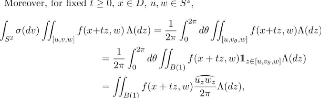
We consider a piecewise-deterministic process of neutron transport with constant velocity. Let D be an open connected bounded domain of R2, let S2 be the unit sphere of R2and σ(du) be the uniform probability measure on S2.
We consider the Markov process (Xt, Vt)t≥0in D×S2constructed as follows:
Xt=R0tVsds and the velocity Vt∈ S2 is a pure jump Markov process, with
constant jump rate λ > 0 and uniform jump probability distribution σ. In other words, Vt jumps to i.i.d. uniform values in S2 at the jump times of a
Poisson process. At the first time where Xt 6∈ D, the process immediately
jumps to the cemetery point ∂, meaning that the process is absorbed at the boundary of D. An example of path of the process (X, V ) is shown in Fig. 1. For all x ∈ D and u ∈ S2, we denote by Px,u (resp. Ex,u) the distribution of
(X, V ) conditionned on (X0, V0) = (x, u) (resp. the expectation with respect
to Px,u).
Remark 5. The assumptions of contant velocity, uniform jump distribution, uniform jump rates and on the dimension of the process can be relaxed but we restrict here to the simplest case to illustrate how conditions (A1) and (A2) can be checked. In particular, it is easy to extend our results to variants of the process where, for instance, the jump measure for V may depend on the state of the process, provided this measure is absolutely continuous w.r.t. σ with density uniformly bounded from above and below. We denote by ∂D the boundary of the domain D, diam(D) its diameter, and for all A ⊂ R2 and x ∈ R2, by d(x, A) the distance of x to the set A: d(x, A) = infy∈A|x − y|. We also denote by B(x, r) the open ball of R2
centered at x with radius r. We assume that the domain D is connected and smooth enough, in the following sense.
Assumption (B) We assume that there exists ε > 0 such that (B1) Dε:= {x ∈ D : d(x, ∂D) > ε} is non-empty and connected;
X0 V0 XJ1 VJ1 XJ5 VJ5 ∂ ∂D
Figure 1: A sample path of the neutron transport process (X, V ). The times J1< J2< . . . are the successive jump times of V .
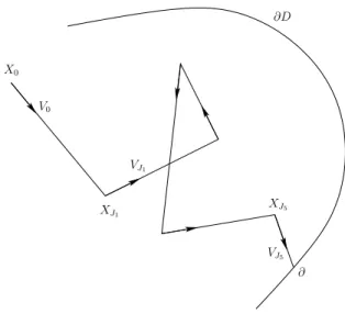
(B2) there exists 0 < sε< tε and σ > 0 such that, for all x ∈ D \ Dε, there
exists Kx ⊂ S2 measurable such that σ(Kx) ≥ σ and for all u ∈ Kx,
x + su ∈ Dε for all s ∈ [sε, tε] and x + su 6∈ ∂D for all s ∈ [0, sε].
As illustrated by Fig. 2, assumption (B2) means that, for all x ∈ D \ Dε,
the set Lx := ® y ∈ R2 : |y − x| ∈ [sε, tε] and y − x |y − x| ∈ Kx ´
is included in Dε and has Lebesgue measure larger than σ2(t2ε− s2ε) > 0.
These assumptions are true for example if ∂D is a C2 connected com-pact manifold, since then the so-called interior sphere condition entails the existence of a cone Kx satisfying (B2) provided ε is small enough compared
to the maximum curvature of the manifold.
Theorem 4.3. Assumption (B) implies (i–vi) in Theorem 2.1.
Proof. In all the proof, we will make use of the following notation: for all k ≥ 1, let Jk be the k-th jump time of Vt (the absorption time is not
considered as a jump, so Jk+1= ∞ if Jk< ∞ and Xt hits ∂D after Jk and
before the (k + 1)-th jump of Vt).
Let us first prove (A1). The following properties are easy consequences of the boundedness of D and Assumption (B).
x ∂D Dε Kx Lx sε tε
Figure 2: The sets Kx and Lx of Assumption (B2).
Lemma 4.4. (i) There exists n ≥ 1 and x1, . . . , xn ∈ Dε such that Dε ⊂
Sn
i=1B(xi, ε/16).
(ii) For all x, y ∈ Dε, there exists m ≤ n and i1, . . . , imdistinct in {1, . . . , n}
such that x ∈ B(xi1, ε/16), y ∈ B(xim, ε/16) and for all 1 ≤ j ≤ m−1,
B(xij, ε/16) ∩ B(xij+1, ε/16) 6= ∅.
The next lemma is proved just after the current proof.
Lemma 4.5. For all x ∈ D, u ∈ S2 and t > 0 such that d(x, ∂D) > t, the
law of (Xt, Vt) under Px,u satisfies
Px,u(Xt∈ dz, Vt∈ dv) ≥ λ 2e−λt
4πt
(t − |z − x|)2
t + |z − x| 1z∈B(x,t)Λ(dz)σ(dv), where Λ is Lebesgue’s measure on R2.
This lemma has the following immediate consequence. Fix i 6= j in {1, . . . , n} such that B(xi, ε/16) ∩ B(xj, ε/16) 6= ∅. Then, for all x ∈
B(xi, ε/16) and u ∈ S2,
Px,u(Xε/2∈ dz, Vε/2∈ dv) ≥ Cε1B(xj,ε/8)∪B(xi,ε/8)(z)Λ(dz) σ(dv),
for a constant Cε> 0 independent of x, i and j.
Combining this result with Lemma 4.4, one easily deduces that for all x ∈ Dε, u ∈ S2 and m ≥ n,
where cε = CεΛ(B(ε/16)) = Cεπε2/256. Proceeding similarly, but with a
first time step of length in [ε/2, ε), we can also deduce from Lemma 4.5 that, for all t ≥ nε/2,
Px,u(Xt∈ dz, Vt∈ dv) ≥ Cε′c⌊2t/ε⌋−1ε 1Dε(z)Λ(dz) σ(dv) (4.13)
for a contant Cε′ > 0.
This entails (A1) with ν the uniform probability measure on Dε× S2
and any t0 ≥ nε/2, but only for initial conditions in Dε× S2.
Now, assume that x ∈ D \ Dε and u ∈ S2. Let
s = inf{t ≥ 0 : x + tu ∈ Dε∪ ∂D}.
If x + su ∈ ∂Dε, then Px,u(Xs ∈ ∂Dε) ≥ e−λs ≥ e−λ diam(D), and thus,
combining this with (4.13), for all t > nε/2,
Px,u(Xs+t ∈ dz, Vs+t∈ dv | s + t < τ∂) ≥ Px,u(Xs+t ∈ dz, Vs+t∈ dv) ≥ e−λ diam(D)Cε′c⌊2t/ε⌋−1ε 1Dε(z)Λ(dz) σ(dv). If x + su ∈ ∂D, Px,u(Xtε ∈ Dε, tε< τ∂) ≥ P(J1 < s ∧ (tε− sε), VJ1 ∈ Kx+uJ1, J2 > tε) ≥ σe−λtεP(J 1 < s ∧ (tε− sε)).
Hence (4.13) entails, for all t ≥ nε/2 such that t + tε≥ s,
Px,u(Xtε+t ∈ dz, Vtε+t ∈ dv | tε+ t < τ∂) ≥ Px,u(Xtε ∈ Dε, tε< τ∂, Xtε+t ∈ dz, Vtε+t ∈ dv) Px,u(t + tε< τ∂) ≥ P(J1 < s ∧ (tε− sε)) P(J1 < s) σe−λtεc⌊2t/ε⌋+1 ε 1Dε(z)Λ(dz) σ(dv).
Since tε≤ diam(D), we have for all 0 < s ≤ diam(D)
P(J1 < s ∧ (tε− sε))
P(J1 < s)
≥ 1 − e
−λ(tε−sε)
1 − e−λ diam(D) > 0.
Hence, we have proved (A1) with ν the uniform probability measure on Dε× S2 and t0 = nε2 + diam(D).
Now we come to the proof of (A2). This can be done in two steps: first, we prove that for all x ∈ D and u ∈ S2,
for some constant C independent of x and u; second
Pν(J1 < ∞, XJ1 ∈ dz) ≥ c1D(z)Λ(dz) (4.15)
for some constant c > 0.
Since for all k ≥ 1, conditionally on {Jk < ∞}, VJk is uniformly
dis-tributed on S2 and independent of XJk, this is enough to conclude as
fol-lows: by (4.14) and the inequality J4 ≤ 4 diam(D) a.s. on τ∂ > t, for all
t ≥ 4 diam(D),
Px,u(t < τ∂) ≤ Ex,u[PXJ4,VJ4(t − 4 diam(D) < τ∂)]
≤ C Z Z D Z S2 Pz,v(t − 4 diam(D) < τ∂)σ(dv)Λ(dz).
Similarly, (4.15) entails that, for all t ≥ diam(D), Pν(t < τ∂) ≥ c Z Z D Z S2 Pz,v(t < τ∂)σ(dv)Λ(dz),
and thus, for all t ≥ 5 diam(D), Px,u(t < τ∂) ≤
C
cPν(t − 4 diam(D) < τ∂).
Now, it follows from (A1) that Pν((Xt0, Vt0) ∈ ·) ≥ c1Pν(t0 < τ∂)ν(·) and
thus
Pν(t − 4 diam(D) + t0 < τ∂) = Eν[PXt0,Vt0(t − 4 diam(D) < τ∂)]
≥ c1Pν(t − 4 diam(D) < τ∂).
Iterating this inequality as needed completes the proof of (A2).
So it only remains to prove (4.14) and (4.15). We start with (4.14). We denote by ( ˆXt, ˆVt)t≥0 the neutron transport process in ˆD = R2, coupled
with (X, V ) such that ˆXt = Xt and ˆVt = Vt for all t < τ∂. We denote by
ˆ
J1 < ˆJ2 < . . . the jumping times of ˆV . It is clear that ˆJk= Jk for all k ≥ 1
such that Jk< ∞.
Now, ˆXJˆ4 = Y1+ Y2+ Y3+ Y4, where the r.v. Y1, . . . , Y4are independent,
Y1 = x + uZ, where Z is an exponential r.v. of parameter λ, and Y2, Y3, Y4
are all distributed as V Z, where V is uniform on S2 and independent of Z. Using the change of variable from polar to Cartesian coordinates, one checks that V Z has density g(z) = λe2π|z|−λ|z| w.r.t. Λ(dz), so that g ∈ L3/2(R2).
Applying twice Young’s inequality, one has g ∗ g ∗ g ∈ L∞(R2). Hence, for all f ∈ B(R2), Ex,u[f (XJ4); J4< τ∂] ≤ E[f ( ˆXJˆ4)] ≤ kg ∗ g ∗ gk∞ Z Z R2f (z)Λ(dz). Hence (4.14) is proved.
We finally prove (4.15). For all x, y ∈ R2, we denote by [x, y] the segment delimited by x and y. For all f ∈ B(R2),
Eν[f (XJ1); J1 < ∞] = Z Z Dε Λ(dx) Λ(Dε) Z S2σ(du) Z ∞ 0 1[x,x+su]⊂D λe−λsf (x + su) ds = Z Z Dε Λ(dx) Λ(Dε) Z Z DΛ(dz)1[x,z]⊂D λe−λ|z−x| 2π|z − x|f (z) ≥ λe −λ diam(D) 2πdiam(D)Λ(Dε) Z Z D Λ(dz)f (z) Z Z Dε Λ(dx)1[x,z]⊂D.
Now, for all z ∈ D \ Dε, using assumption (B2),
Z Z Dε 1[x,z]⊂DΛ(dx) ≥ Λ(Lz) ≥ σ 2(t 2 ε− s2ε),
and for all z ∈ Dε,
Z Z
Dε
1[x,z]⊂DΛ(dx) ≥ Λ(Dε∩ B(z, ε)).
Since the map z 7→ Λ(Dε∩B(z, ε)) is continuous and positive on the compact
set Dε, we have proved (4.15).
Proof of Lemma 4.5. Using twice the relation: for all bounded measurable f , k ≥ 1, t ≥ 0, x ∈ D and u ∈ S2, Ex,u[f (Xt, Vt); Jk≤ t < Jk+1] = Z t 0 dsλe −λsZ S2σ(dv)Ex+su,v[f (Xt−s, Vt−s); Jk−1≤ t − s < Jk], we obtain Ex,u[f (Xt, Vt); J2≤ t < J3] = λ2e−λt Z S2σ(dv) Z S2σ(dw) Z t 0 ds Z t−s 0 dθf (x + su + θv + (t − s − θ)w, w).
For all x, y, z ∈ R2, we denote by [x, y, z] the triangle of R2 delimited by x, y and z. Using the well-known fact that a point in [x, y, z] with barycentric coordinates distributed uniformly on the simplex is distributed uniformly on [x, y, z], we deduce that Ex,u[f (Xt, Vt); J2≤ t < J3] = λ 2t2 2 e −λtZ S2σ(dv) Z S2σ(dw) Z Z [u,v,w] f (x + tz, w) Λ(dz) Λ([u, v, w]). Now, for all u, v, w ∈ S2,
Λ([u, v, w]) = 1
2|u − w| |v − v
′| ≤ |u − w|,
where v′ is the orthogonal projection of v on the line (u, w) (see fig. 3), and
where we used the fact that |v − v′| ≤ 2.
Moreover, for fixed t ≥ 0, x ∈ D, u, w ∈ S2, Z S2σ(dv) Z Z [u,v,w] f (x+tz, w) Λ(dz) = 1 2π Z 2π 0 dθ Z Z [u,vθ,w] f (x+tz, w)Λ(dz) = 1 2π Z 2π 0 dθ Z Z B(1)f (x + tz, w)1z∈[u,vθ,w] Λ(dz) = Z Z B(1) f (x + tz, w)u˘zwz 2π Λ(dz),
where vθ = (cos θ, sin θ) ∈ R2, B(r) is the ball centered at 0 of radius r of
R2, uz (resp. wz) is the symmetric of u (resp. w) with respect to z in S2
(see Fig. 4) anduv is the length of the arc between u and v in Sı 2.
u w u0 w0 uz wz z z0 S2 δ ˙ uzwz
Figure 4: Definition of uz, wz,u˘zwz, z0, u0 and w0. The angle marked M is
larger than the one marked ).
Fix 0 < δ < 1, and let z0 be the farthest point in B(δ) from {u, w}
(this point is unique except when the segment [u, w] between u and w is a diameter of S2). We set u0 = uz0 and w0 = wz0 (see Fig. 4). Note that
Thales’ theorem implies that
|u0− w0| =
1 − δ
Then, for any z ∈ B(δ), we have uz’0w ≤ uzw, where‘ ‘xyz is the measure
of the angle formed by the segments [y, x] and [y, z]. Since in addition |z0− u0| = |z0− w0| ≤ 1 and |z − uz| ∧ |z − wz| ≥ 1 − δ, Thales’ theorem
yields
|uz− wz|
1 − δ ≥ |u0− w0|. Puting everything together, we deduce that
Ex,u[f (Xt, Vt);J2≤ t < J3] ≥ λ 2t2 4π e −λtZ S2 σ(dw) Z Z B(1) f (x + tz, w)|uz− wz| |u − w| Λ(dz) ≥ λ 2t2 4π e −λtZ S2σ(dw) Z Z B(1)f (x + tz, w) (1 − |z|)2 1 + |z| Λ(dz). This ends the proof of Lemma 4.5.
5
Quasi-stationary distribution: proofs of the
re-sults of Section 2
This section is devoted to the proofs of Theorem 2.1 (Sections 5.1 and 5.2), Corollary 2.2 (Section 5.3), Proposition 2.3 (Section 5.4) and Corollary 2.4 (Section 5.5). In Theorem 2.1, the implications (iii)⇒(i)⇒(ii) and (iv)⇒(v)⇒(vi) are obvious so we only need to prove (ii)⇒(iv) and (vi)⇒(iii).
5.1 (ii) implies (iv)
Assume that X satisfies Assumption (A’). We shall prove the result assuming (A1’) holds for t0= 1. The extension to any t0 is immediate.
Step 1: control of the distribution at time 1, conditionally on non-absorption at a later time.
Let us show that, for all t ≥ 1 and for all x1, x2 ∈ E, there exists a probability
measure νxt1,x2 on E such that, for all measurable set A ⊂ E,
Pxi(X1 ∈ A | t < τ∂) ≥ c1c2νxt1,x2(A), for i = 1, 2. (5.1)
Fix x1, x2 ∈ E, i ∈ {1, 2}, t ≥ 1 and a measurable subset A ⊂ E. Using the
Markov property, we have
Pxi(X1 ∈ A and t < τ∂) = Exi[1A(X1)PX1(t − 1 < τ∂)]
= Exi[1A(X1)PX1(t − 1 < τ∂) | 1 < τ∂] Pxi(1 < τ∂)
by Assumption (A1’). Dividing both sides by Pxi(t < τ∂), we deduce that
Pxi(X1 ∈ A | t < τ∂) ≥ c1νx1,x2(1A(·)P·(t − 1 < τ∂))
Pxi(1 < τ∂)
Pxi(t < τ∂)
. Using again the Markov property, we have
Pxi(t < τ∂) ≤ Pxi(1 < τ∂) sup y∈E Py(t − 1 < τ∂) , so that Pxi(X1∈ A | t < τ∂) ≥ c1νx1,x2(1A(·)P·(t − 1 < τ∂)) supy∈EPy(t − 1 < τ∂) . Now Assumption (A2’) implies that the non-negative measure
B 7→ νx1,x2(1B(·)P·(t − 1 < τ∂))
supy∈EPy(t − 1 < τ∂)
has a total mass greater than c2. Therefore (5.1) holds with
νxt1,x2(B) = νx1,x2(1B(·)P·(t − 1 < τ∂))
Pνx1,x2(t − 1 < τ∂)
Step 2: exponential contraction for Dirac initial distributions We now prove that, for all x, y ∈ E and T ≥ 0
kPx(XT ∈ · | T < τ∂) − Py(XT ∈ · | T < τ∂)kT V ≤ 2(1 − c1c2)⌊T ⌋. (5.2)
Let us define, for all 0 ≤ s ≤ t ≤ T the linear operator RTs,t by RTs,tf (x) = Ex(f (Xt−s) | T − s < τ∂)
= E(f (Xt) | Xs= x, T < τ∂),
by the Markov property. For any T > 0, the family (Rs,tT )0≤s≤t≤T is a
Markov semi-group: we have, for all 0 ≤ u ≤ s ≤ t ≤ T and all bounded measurable function f ,
RTu,s(RTs,tf )(x) = RTu,tf (x).
This can be proved as Lemma 12.2.2 in [15] or by observing that a Markov process conditioned by an event in its tail σ-field remains Markovian (but no longer time-homogeneous).
For any x1, x2 ∈ E, we have by (5.1) that δxiR
T
s,s+1− c1c2νxT −s1,x2 is a
positive measure whose mass is 1 − c1c2, for i = 1, 2. We deduce that
δx1R T s,s+1− δx2R T s,s+1 T V ≤ kδx1R T s,s+1− c1c2νxT −s1,x2kT V + kδx2R T s,s+1− c1c2νxT −s1,x2kT V ≤ 2(1 − c1c2).
Let µ1, µ2 be two mutually singular probability measures on E and any
f ≥ 0, we have µ1R T s,s+1− µ2RTs,s+1 T V ≤ Z Z E2 δxR T s,s+1− δyRTs,s+1 T V dµ1⊗ dµ2(x, y) ≤ 2(1 − c1c2) = (1 − c1c2)kµ1− µ2kT V.
Now if µ1 and µ2 are any two different probability measures (not
neces-sarily mutually singular), one can apply the previous result to the mutually singular probability measures (µ1−µ2)+
(µ1−µ2)+(E) and (µ1−µ2)− (µ1−µ2)−(E). Then (µ1− µ2)+ (µ1− µ2)+(E)R T s,s+1− (µ1− µ2)− (µ1− µ2)−(E)R T s,s+1 T V ≤ (1 − c1c2) (µ1− µ2)+ (µ1− µ2)+(E) − (µ1− µ2)− (µ1− µ2)−(E) T V . Since µ1(E) = µ2(E) = 1, we have (µ1− µ2)+(E) = (µ1 − µ2)−(E). So
multiplying the last inequality by (µ1− µ2)+(E), we deduce that
k(µ1− µ2)+RTs,s+1− (µ1− µ2)−Rs,s+1T kT V
≤ (1 − c1c2)k(µ1− µ2)+− (µ1− µ2)−kT V.
Since (µ1− µ2)+− (µ1− µ2)− = µ1− µ2, we obtain
kµ1RTs,s+1− µ2RTs,s+1kT V ≤ (1 − c1c2)kµ1− µ2kT V.
Using the semi-group property of (RT
s,t)s,t, we deduce that, for any x, y ∈ E,
kδxRT0,T − δyRT0,TkT V = kδxRT0,T −1RTT −1,T − δyRT0,T −1RTT −1,TkT V
≤ (1 − c1c2) kδxRT0,T −1− δyRT0,T −1kT V
By definition of RT0,T, this inequality immediately leads to (5.2). Step 3: exponential contraction for general initial distributions
We prove now that inequality (5.2) extends to any pair of initial probability measures µ1, µ2 on E, that is, for all T ≥ 0,
kPµ1(XT ∈ · | T < τ∂) − Pµ2(XT ∈ · | T < τ∂)kT V ≤ 2(1 − c1c2)
⌊T ⌋. (5.3)
Let µ1 be a probability measure on E and x ∈ E. We have
kPµ1(XT ∈ · | T < τ∂) − Px(XT ∈ · | T < τ∂)kT V = 1 Pµ1(T < τ∂) kPµ1(XT ∈ ·) − Pµ1(T < τ∂)Px(XT ∈ · | T < τ∂)kT V ≤ 1 Pµ1(T < τ∂) Z y∈EkPy (XT ∈ ·) − Py(T < τ∂)Px(XT ∈ · | T < τ∂)kT Vdµ1(y) ≤ 1 Pµ1(T < τ∂) Z y∈E Py(T < τ∂)kPy(XT ∈ · | T < τ∂) − Px(XT ∈ · | T < τ∂)kT Vdµ1(y) ≤ 1 Pµ1(T < τ∂) Z y∈E Py(T < τ∂)2(1 − c1c2)⌊T ⌋dµ1(y) ≤ 2(1 − c1c2)⌊T ⌋.
The same computation, replacing δx by any probability measure, leads
to (5.3).
Step 4: existence and uniqueness of a quasi-stationary distribution for X. Let us first prove the uniqueness of the quasi-stationary distribution. If α1
and α2 are two quasi-stationary distributions, then we have Pαi(Xt∈ ·|t <
τ∂) = αi for i = 1, 2 and any t ≥ 0. Thus, we deduce from inequality (5.3)
that
kα1− α2kT V ≤ 2(1 − c1c2)⌊t⌋, ∀t ≥ 0,
which yields α1 = α2.
Let us now prove the existence of a QSD. By [28, Proposition 1], this is equivalent to prove the existence of a quasi-limiting distribution for X. So we only need to prove that Px(Xt ∈ ·|t < τ∂) converges when t goes to
infinity, for some x ∈ E. We have, for all s, t ≥ 0 and x ∈ E, Px(Xt+s ∈ · | t + s < τ∂) = δxPt+s δxPt+s1E = δxPtPs δxPtPs1E = δxR s 0,sPt δxRs0,sPt1E = PδxRs0,s(Xt∈ · | t < τ∂) , (5.4)
where we use the identity Rs
0,sf (x) = PPss1f (x)E(x) for the third equality. Hence
kPx(Xt∈ ·|t < τ∂) − Px(Xt+s∈ ·|t + s < τ∂)kT V
= kPx(Xt∈ ·|t < τ∂) − PδxRs0,s(Xt∈ ·|t < τ∂)kT V
≤ 2 (1 − c1c2)⌊t⌋−−−−−→ s,t→+∞ 0.
In particular the sequence (Px(Xt∈ · | t < τ∂))t≥0 is a Cauchy sequence for
the total variation norm. The space of probability measures on E equipped with the total variation norm is complete, so Px(Xt ∈ · | t < τ∂) converges
when t goes to infinity to some probability measure α on E.
Finally Equation (2.3) follows from (5.3) with µ1 = µ and µ2 = α.
Therefore we have proved (iv) and the last statement of Theorem 2.1 con-cerning existence and uniqueness of a quasi-stationary distribution and the explicit expression for C and γ.
5.2 (vi) implies (iii)
Assume that (2.2) holds with some probability measure α on E. Let us define
ε(t) = sup
x∈EkPx
(Xt∈ · | t < τ∂) − αkT V .
Step 1: ε(·) is non-increasing and α is a quasi-stationary distribution For all s, t ≥ 0, x ∈ E and A ∈ E,
|Px(Xt+s ∈ A | t + s < τ∂) − α(A) = Ex{1t<τ∂PXt(s < τ∂) [PXt(Xs∈ A | s < τ∂) − α(A)]} Px(t + s < τ∂) ≤ Ex{1t<τ∂PXt(s < τ∂) |PXt(Xs∈ A | s < τ∂) − α(A)|} Px(t + s < τ∂) ≤ ε(s).
Taking the supremum over x and A, we deduce that the function ε(·) is non-increasing. By (2.2), this implies that ε(t) goes to 0 when t → +∞. By Step 4 above, α is a quasi-stationary distribution and there exists λ0 > 0
Step 2: proof of (A2′′) for µ = α We define, for all s ≥ 0,
A(s) = supx∈EPx(s < τ∂) Pα(s < τ∂).
= eλ0ssup
x∈E
Px(s < τ∂).
Our goal is to prove that A is bounded. The Markov property implies, for s ≤ t,
Px(t < τ∂) = Px(s < τ∂) E (PXs(t − s < τ∂) | s < τ∂) .
By (2.2), the total variation distance between α and Lx(Xs | s < τ∂) is
smaller than ε(s), so Px(t < τ∂) ≤ Px(s < τ∂) Ç Pα(t − s < τ∂) + ε(s) sup y∈E Py(t − s < τ∂) å . For s ≤ t, we thus have
A(t) ≤ A(s) (1 + ε(s)A(t − s)) . (5.5) The next lemma proves that
Pα(t < τ∂) = e−λ0t≥ c2(α) sup x∈E
Px(t < τ∂) (5.6)
for the constant c2(α) = 1/ sups>0A(s) and concludes Step 2.
Lemma 5.1. A function A : R+ 7→ R+ satisfying (5.5) for all s ≤ t is
bounded.
Proof. We introduce the non-decreasing function ψ(t) = sup0≤s≤tAs. It
follows from (5.5) that, for all s ≤ u ≤ t,
A(u) ≤ ψ(s) (1 + ε(s)ψ(t − s)) .
Since this inequality holds also for u ≤ s, we obtain for all s ≤ t,
ψ(t) ≤ ψ(s) (1 + ε(s)ψ(t − s)) . (5.7) By induction, for all N ≥ 1 and s ≥ 0,
ψ(N s) ≤ ψ(s) N −1 Y k=1 (1 + ε(ks)ψ(s)) ≤ ψ(s) exp ψ(s) N −1 X k=1 ε(ks) ! ≤ ψ(s) exp ψ(s) ∞ X k=1 ε(ks) ! , (5.8)
whereP∞
k=1ε(ks) < ∞ by (2.2).
Since ψ is non-decreasing, it is bounded.
Remark 6. Note that, under Assumption (v), ε(t) ≤ Ce−γt. Using the fact
that ψ(s) ≤ eλ0s, we deduce from (5.8) that, for all s > 0,
A(N s) ≤ exp Ç λ0s + Ce(λ0−γ)s 1 − e−γs å . This justifies (2.5) in Remark 1.
Step 3: proof of (A2′′)
Applying Step 3 of Section 5.1 with µ1 = ρ and δx= α, we easily obtain
ε(t) = sup
ρ∈M1(E)
kPρ(Xt∈ · | t < τ∂) − αkT V .
Let µ be a probability measure on E. For any s ≥ 0, let us define µs(·) =
Pµ(Xs∈ · | s < τ∂). We have kµs− αkT V ≤ ε(s) and so Pµs(t − s < τ∂) ≥ Pα(t − s < τ∂) − ε(s) sup x∈E Px(t − s < τ∂) ≥ e−λ0(t−s)− ε(s) c2(α) e−λ0(t−s)
by (5.6). Since ε(s) decreases to 0, there exists s0 such that ε(s0)/c2(α) =
1/2. Using the Markov property, we deduce that, for any t ≥ s0,
Pµ(t < τ∂) = Pµs0(t − s0 < τ∂)Pµ(s0 < τ∂)
≥ e
−λ0(t−s0)
2 Pµ(s0 < τ∂). Therefore, by (5.6), we have proved that
Pµ(t < τ∂) ≥ c2(µ) sup x∈E Px(t < τ∂) for c2(µ) = 1 2c2(α)e λ0s0P µ(s0 < τ∂) > 0.
Step 4: construction of the measure ν in (A1)
We define the measure ν as the infimum of the family of measures (δxR2t0,2t)x∈E,
as defined in the next lemma, for a fixed t such that c2(α) ≥ 2ε(t). To prove
Lemma 5.2. Let (µx)x∈F be a family of positive measures on E indexed by
an arbitrary set F . For all A ∈ E, we define µ(A) = inf ( n X i=1 µxi(Bi) | n ≥ 1, x1, . . . , xn∈ F, B1, . . . , Bn∈ E partition of A ) . Then µ is the largest non-negative measure on E such that µ ≤ µx for all
x ∈ F and is called the infimum measure of (µx)x∈F.
Proof of Lemma 5.2. Clearly µ(A) ≥ 0 for all A ∈ E and µ(∅) = 0. Let us prove the σ-additivity. Consider disjoints measurable sets A1, A2, . . . and
define A = ∪kAk. Let B1, . . . , Bn be a measurable partition of A. Then n X i=1 µxi(Bi) = ∞ X k=1 n X i=1 µxi(Bi∩ Ak) ≥ ∞ X k=1 µ(Ak). Hence µ(A) ≥P∞ k=1µ(Ak).
Fix K ≥ 1 and ǫ > 0. For all k ∈ {1, . . . , K}, let (Bki)i∈{1,...,nk} be a
partition of Ai and (xki)i∈{1,...,nk} be such that
µ(Ak) ≥ nk X i=1 µxk i(B k i) − ǫ 2k. Then K X k=1 µ(Ak) ≥ K X k=1 nk X i=1 µxk i(B k i) − ǫ 2k ! ≥ µ K [ k=1 Ak ! − ǫ. Since, for any x0 ∈ F ,
µ(A) ≤ µ K [ k=1 Ak ! + µx0 A \ K [ k=1 Ak ! ,
choosing K large enough, µ(A) ≤ µÄ∪K k=1Ak
ä
+ ǫ. Combining this with the previous inequality, we obtain
µ(A) ≥
∞
X
k=1
µ(Ak) ≥ µ(A) − 2ǫ.
Let us now prove that µ is the largest non-negative measure on E such that µ ≤ µxfor all x ∈ F . Let ˆµ be another measure such that ˆµ ≤ µx. Then,
for all A ∈ E and B1, . . . , Bna measurable partition of A and x1, . . . , xn∈ F ,
ˆ µ(A) = n X i=1 ˆ µ(Bi) ≤ n X i=1 µxi(Bi).
Taking the infimum over (Bi) and (xi) implies that ˆµ ≤ µ.
Let us now prove that ν is a positive measure. By (5.4), for any x ∈ E, t ≥ 0 and A ⊂ E measurable, δxR2t0,2t(A) = PδxRt0,t(Xt∈ A|t < τ∂) = R EPy(Xt∈ A)δxRt0,t(dy) R EPy(t < τ∂)δxRt0,t(dy) . By Step 2, we have δxR2t0,2t(A) ≥ c2(α)eλ0t Z E Py(Xt∈ A)δxRt0,t(dy).
We set νt,x+ = (α − δxRt0,t)+. Using the inequality (between measures)
δxRt0,t ≥ α − νt,x+,
δxR2t0,2t(A) ≥ c2(α)α(A) − c2(α)eλ0t
Z
E
Py(Xt∈ A | t < τ∂)Py(t < τ∂)νt,x+(dy).
Since νt,x+ is a positive measure, Step 2 implies again
δxR2t0,2t(A) ≥ c2(α)α(A) − Z E Py(Xt∈ A | t < τ∂)νt,x+(dy) = c2(α)α(A) − Z E δyRt0,t(A)νt,x+(dy) ≥Äc2(α) − νt,x+(E) ä α(A) − Z E Ä δyRt0,t(A) − α(A) ä νt,x+(dy) ≥ (c2(α) − ε(t)) α(A) − Z E Ä δyRt0,t(A) − α(A) ä +ν + t,x(dy),
where the inequality νt,x+(E) ≤ ε(t) follows from (2.2). Moreover νt,x+ = (α − δxRt0,t)+≤ α, therefore δxR2t0,2t(A) ≥ (c2(α) − ε(t)) α(A) − Z E Ä δyR0,tt (A) − α(A) ä +α(dy).
Hence, for all B1, . . . , Bna measurable partition of E and all x1, . . . , xn∈ E, n X i=1 δxiR 2 0,2tt(Bi) ≥ (c2(α) − ε(t)) α(E) − Z E n X i=1 Ä δyR0,tt (Bi) − α(Bi) ä +α(dy). Now n X i=1 Ä δyRt0,t(Bi) − α(Bi) ä +≤ δyR t 0,t(Bi) − α(Bi) T V ≤ ε(t). Therefore ν(E) ≥ c2(α) − 2ε(t) > 0.
This concludes the proof of Theorem 2.1. 5.3 Proof of Corollary 2.2
Assume that the hypotheses of Theorem 2.1 are satisfied and let µ1, µ2 be
two probability measures and t ≥ 0. Without loss of generality, we assume that Pµ1(t < τ∂) ≥ Pµ2(t < τ∂) and prove that
kPµ1(Xt∈ · | t < τ∂) − Pµ2(Xt∈ · | t < τ∂)k ≤
(1 − c1c2)⌊t/t0⌋
c2(µ1) kµ1− µ2kT V
. Using the relation
µ1Pt= (µ1− (µ1− µ2)+)Pt+ (µ1− µ2)+Pt,
the similar one for µ2Ptand µ1− (µ1− µ2)+= µ2− (µ2− µ1)+, we can write
µ1Pt
µ1Pt1E −
µ2Pt
µ2Pt1E
= α1Pt− α2Pt, (5.9)
where α1 and α2 are the positive measures defined by
α1 = (µ1− µ2)+ µ1Pt1E and α2= (µ2− µ1)+ µ2Pt1E + Å 1 µ2Pt1E − 1 µ1Pt1E ã × (µ1− (µ1− µ2)+) .
We immediately deduce from(5.9), that α1Pt1E = α2Pt1E, so that
kα1Pt− α2PtkT V = α1Pt1E α1 α1Pt1E Pt− α2 α2Pt1E Pt T V ≤ 2(1 − c1c2)⌊t/t0⌋α1Pt1E.
Since α1Pt1E = (µ1− µ2)+Pt1E µ1Pt1E ≤ (µ1− µ2)+(E) supρ∈M1(E)ρPt1E µ1Pt1E ≤ kµ1− µ2kT V 2c2(µ1)
by definition of c2(µ1), the proof of Corollary 2.2 is complete.
5.4 Proof of Proposition 2.3 Step 1: Existence of η.
For all x ∈ E and t ≥ 0, we set ηt(x) =
Px(t < τ∂)
Pα(t < τ∂)
= eλ0tP
x(t < τ∂).
By the Markov property
ηt+s(x) = eλ0(t+s)Ex(1t<τ∂PXt(s < τ∂))
= ηt(x)Ex(ηs(Xt) | t < τ∂) .
By (A2′′), R
Eηs(y)ρ(dy) is uniformly bounded by 1/c2(α) in s and in ρ ∈
M1(E). Therefore, by (2.1), |Ex(ηs(Xt) | t < τ∂) − α(ηs)| ≤ C c2(α) e−γt. Since, α(ηs) = 1, we obtain sup x∈E|ηt+s (x) − ηt(x)| ≤ C c2(α)2 e−γt.
That implies that (ηt)t≥0is a Cauchy family for the uniform norm and hence
converges uniformly to a bounded limit η. By Lebesgue’s theorem, α(η) = 1. It only remains to prove that η(x) > 0 for all x ∈ E. This is an immediate consequence of (A2′′).
Step 2: Eigenfunction of the infinitesimal generator.
We prove now that η belongs to the domain of the infinitesimal generator L of the semi-group (Pt)t≥0 and that
For any h > 0, we have by the dominated convergence theorem and Step 1, Phη(x) = Ex(η(Xh)) = lim t→∞ Ex(PXh(t < τ∂)) Pα(t < τ∂) .
We have Pα(t < τ∂) = e−λ0hPα(t + h < τ∂). Hence, by the Markov property,
Phη(x) = lim t→∞e
−λ0hPx(t + h < τ∂)
Pα(t + h < τ∂)
= e−λ0hη(x).
Since η is uniformly bounded, it is immediate that Phη − η
h
k·k∞
−−−→
h→0 −λ0η.
By definition of the infinitesimal generator, this implies that η belongs to the domain of L and that (5.10) holds.
5.5 Proof of Corollary 2.4
Since Lf = λf , we have Ex(f (Xt)) = Ptf (x) = eλtf (x). When f (∂) 6= 0,
taking x = ∂, we see that λ = 0 and, taking x 6= ∂, the left hand side converges to f (∂) and thus f is constant. So let us assume that f (∂) = 0. By property (v),
Ptf (x)
Pt1E(x)− α(f ) −−−−→t→+∞
0
uniformly in x ∈ E and exponentially fast. Assume first that α(f ) 6= 0, then by Proposition 2.3,
e(λ+λ0)tf (x)
η(x) −−−−→t→+∞ α(f ), ∀x ∈ E.
We deduce that λ = −λ0 and f (x) = α(f )η(x) for all x ∈ E ∪ {∂}. Assume
finally that α(f ) = 0, then, using (2.4) to give a lower bound for 1/Pt1E(x),
we deduce that c2(α)e(γ+λ+λ0)tf (x) ≤ eγtP tf (x) Pt1E(x) , ∀x ∈ E,
where the right hand side is bounded by property (v) of Theorem 2.1. Thus γ + λ + λ0 ≤ 0.
![Figure 3: The triangle [u, v, w] and the point v ′ .](https://thumb-eu.123doks.com/thumbv2/123doknet/13375585.404216/28.918.199.716.296.451/figure-triangle-u-v-w-point-v.webp)