HAL Id: hal-01774642
https://hal.archives-ouvertes.fr/hal-01774642v3
Submitted on 10 Oct 2019
HAL is a multi-disciplinary open access
archive for the deposit and dissemination of
sci-entific research documents, whether they are
pub-lished or not. The documents may come from
teaching and research institutions in France or
abroad, or from public or private research centers.
L’archive ouverte pluridisciplinaire HAL, est
destinée au dépôt et à la diffusion de documents
scientifiques de niveau recherche, publiés ou non,
émanant des établissements d’enseignement et de
recherche français ou étrangers, des laboratoires
publics ou privés.
matrix formats: the multilevel BLR format
Patrick Amestoy, Alfredo Buttari, Jean-Yves l’Excellent, Théo Mary
To cite this version:
Patrick Amestoy, Alfredo Buttari, Jean-Yves l’Excellent, Théo Mary. Bridging the gap between
flat and hierarchical low-rank matrix formats: the multilevel BLR format. SIAM Journal on
Sci-entific Computing, Society for Industrial and Applied Mathematics, 2019, 41 (3), pp.A1414-A1442.
�10.1137/18M1182760�. �hal-01774642v3�
PATRICK R. AMESTOY†, ALFREDO BUTTARI‡, JEAN-YVES L’EXCELLENT§,ANDTHEO MARY¶
Abstract. Matrices possessing a low-rank property arise in numerous scientific applications. This property can be
exploited to provide a substantial reduction of the complexity of their LU or LDLTfactorization. Among the possible low-rank formats, the flat Block Low-Rank (BLR) format is easy to use but achieves superlinear complexity. Alternatively, the hierarchical formats achieve linear complexity at the price of a much more complex, hierarchical matrix representation. In this paper, we propose a new format based on multilevel BLR approximations: the matrix is recursively defined as a BLR matrix whose full-rank blocks are themselves represented by BLR matrices. We call this format multilevel BLR (MBLR). Contrarily to hierarchical matrices, the number of levels in the block hierarchy is fixed to a given constant; while this format can still be represented within theH formalism, we show that applying theHtheory to it leads to very pessimistic complexity bounds. We therefore extend the theory to prove better bounds, and show that the MBLR format provides a simple way to finely control the desired complexity of dense factorizations. By striking a balance between the simplicity of the BLR format and the low complexity of the hierarchical ones, the MBLR format bridges the gap between flat and hierarchical low-rank matrix formats. The MBLR format is of particular relevance in the context of sparse direct solvers, for which it is able to trade off the optimal dense complexity of the hierarchical formats to benefit from the simplicity and flexibility of the BLR format while still achieving O(n) sparse complexity. We finally compare our MBLR format with the related BLR-H (or Lattice-H) format; our theoretical analysis shows that both formats achieve the same asymptotic complexity for a given top level block size.
Key words. low-rank approximations, matrix factorization, sparse linear algebra, hierarchical matrices
AMS subject classifications. 15a06, 15a23, 65f05, 65f50, 65n30, 65y20
1. Introduction. Efficiently computing the solution of a dense linear system is a fundamental
building block of numerous scientific computing applications. Let us refer to such a system as
F uF= vF, (1.1)
where F is a dense matrix of order m, uF is the unknown vector of size m, and vFis the right-hand
side vector of size m.
This paper focuses on solving (1.1) with direct approaches based on Gaussian elimination, which consist in factorizing matrix F as F = LU or F = LDLT, depending on whether the matrix is unsymmetric or symmetric, respectively.
In many applications (e.g., Schur complements arising from the discretization of elliptic partial differential equations), the matrix F has been shown to have a low-rank property: many of its off-diagonal blocks can be approximated by low-rank matrices [10].
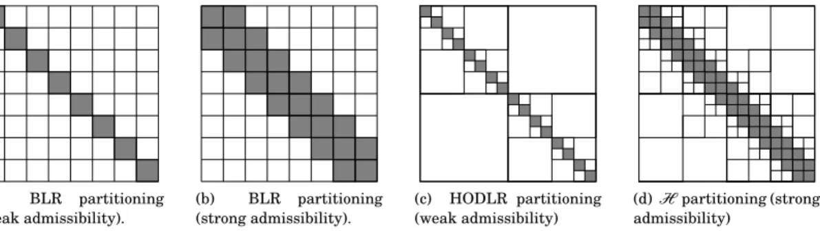
Several formats have been proposed to exploit this property. The simplest one is the Block Low-Rank (BLR) format [2], which partitions the matrix with a flat, 2D blocking and approximates its off-diagonal blocks by low-rank submatrices, as illustrated in Figure1.1a. Compared with the cubic O(m3) complexity of the dense full-rank LU or LDLT factorizations, the complexity of the dense BLR factorization can be as low as O(m2) [4].
More advanced formats are based on a hierarchical partitioning of the matrix: the matrix F is partitioned with a 2 × 2 blocking and the two diagonal blocks are recursively refined, as illustrated in Figures1.1c and 1.1d. Different hierarchical formats can be defined depending on whether the off-diagonal blocks are directly approximated (so-called weakly-admissible formats) or further refined (so-called strongly-admissible formats). The most general of the hierarchical formats is the strongly-admissibleH -matrix format [10,21,12]; the HODLR format [6] is its weakly-admissible counterpart. These hierarchical formats can factorize a dense matrix in near-linear complexity O(m logqm), where q is a small integer that depends on which factorization algorithm is used; in ∗Funding: This work was supported by Engineering and Physical Sciences Research Council grant EP/P020720/1. The
opinions and views expressed in this publication are those of the authors, and not necessarily those of the funding bodies.
†University of Toulouse, INP-IRIT ‡University of Toulouse, CNRS-IRIT
§University of Lyon, CNRS, ENS de Lyon, Inria, UCBL, LIP UMR5668, France
¶School of Mathematics, The University of Manchester, Manchester M13 9PL, UK ([email protected])
(a) BLR partitioning (weak admissibility). (b) BLR partitioning (strong admissibility). (c) HODLR partitioning (weak admissibility) (d)Hpartitioning (strong admissibility)
Fig. 1.1: Illustration of different low-rank formats. Gray blocks are stored in full-rank whereas white ones are approximated by low-rank matrices.
the following, we will consider q = 2. The log factor can be removed by using a so-called nested-basis structure. The strongly-admissibleH2-matrix format [12] and the weakly-admissible HSS [31,13] and HBS [19] formats exploit such nested basis structures to achieve linear complexity O(m).
In this paper, we propose a new format based on multilevel BLR approximations. The matrix F is recursively represented as a BLR matrix whose full-rank blocks are themselves BLR matrices. We call this format multilevel BLR (MBLR). In the hierarchical format, the matrix is refined until the diagonal blocks are of constant size; this therefore leads to a number of levels in the block hierarchy which is nonconstant (usually O(log2m)). With the MBLR format, we propose to make this number of levels a tunable parameter to be set to a given value` that does not asymptotically depend on the matrix size m. We prove that this parameter provides a simple way to finely control the complexity of the dense MBLR factorization. The complexity varies from O(m2) for monolevel BLR down to nearly O(m) for an infinite number of levels. By striking a balance between the simplicity of the BLR format and the low complexity of the hierarchical ones, the MBLR format bridges the gap between flat and hierarchical low-rank matrix formats.
We will show that the MBLR format is of particular relevance in the context of sparse direct solvers, which aim to compute the solution of a sparse linear system
AuA= vA, (1.2)
where A is a sparse matrix of order n, uAis the unknown vector of size n, and vAis the right-hand
side vector of size n. Two widely studied classes of sparse direct methods are the multifrontal [15, 24] and supernodal [9,14] approaches.
Sparse direct methods rely on a sequence of partial factorizations of dense matrices F, referred to as supernodes or fronts. Therefore, the complexity of sparse direct methods is directly derived from the complexity of the factorization of each dense matrix F. For example, with an adequate reordering, a well-known result is that the dense standard full-rank O(m3) factorization leads to a O(n2) sparse complexity for regular 3D problems [16]. The low-rank formats described above can be efficiently exploited within sparse solvers to provide a substantial reduction of their complexity. The potential of BLR sparse solvers has been first investigated in [2]; the simplicity and flexi-bility of the BLR format makes it easy to use in the context of a general purpose, algebraic solver, as presented in [5,3,28,26]. [5] focuses on the multicore performance of BLR multifrontal solvers, while [3] and [28] present their use in two real-life industrial applications coming from geosciences. [26] present the use of the BLR format in supernodal solvers. Furthermore, it has been proved in [4] that the theoretical complexity of the BLR multifrontal factorization may be as low as O(n4/3) (for 3D problems with constant ranks).
Alternatively, most sparse solvers based on the more complex hierarchical formats have been shown to possess near-linear complexity. To cite a few, [30, 29, 18,17] are HSS-based, [19] is HBS-based, [7] is HODLR-based, and [27] isH2-based.
However, a critical observation is that achieving O(n) sparse complexity does not actually require a linear dense complexity O(m). For instance, for 3D problems, all that is required is a
dense complexity lower than O(m1.5). Therefore, we will prove that the MBLR format is able to trade off the optimal dense complexity of the hierarchical formats to benefit from the simplicity and flexibility of the flat BLR format while still achieving O(n) sparse complexity.
We now describe the organization of the rest of this paper. In Section 2, we provide some background on the BLR factorization and its complexity and we motivate the key idea behind MBLR approximations. We explain in Section3how the MBLR format can be described using the cluster tree representation commonly used in theH literature; this provides a convenient way to explain the key difference between the MBLR andH formats. We show that, similarly to the BLR case, theH theoretical formalism leads to MBLR complexity bounds that are very pessimistic. We therefore extend the theory, beginning by the two-level case in Section4. We prove that two levels can already significantly improve the theoretical complexity of the factorization. In Section5, we generalize the previous proof to the MBLR format with an arbitrary number of levels; we prove that, for constant ranks, only four levels are already enough to reach O(n) sparse 3D complexity (and three levels already achieve near-linear O(n log n) complexity). In Section6, we validate our theoretical results with numerical experiments. We provide our concluding remarks in Section7. In the main body of this article, we consider for the sake of simplicity the weakly-admissible case, in which only the diagonal blocks are refined. In the appendix, we provide the extension of the MBLR format to the strongly-admissible case, in which off-diagonal full-rank blocks are also recursively refined. We prove that our complexity bounds remain valid in this context.
2. Background and motivation.
2.1. Block Low-Rank approximations. The BLR format is based on a flat, non-hierarchical
blocking of the matrix which is defined by conveniently clustering the associated unknowns. A BLR representationF of a dense matrix F is shown in (2.1e ), where we assume that p×p blocks have been defined. Off-diagonal blocks Fi j(i 6= j) of size mi× njand numerical rank kεi jare approximated by
a low-rank matrixFei j= Xi jYi jT at accuracyε, where Xi j is a mi× kεi jmatrix and Yi j is a nj× kεi j
matrix. The diagonal blocks Fiiare stored as full-rank matrices (Feii= Fii).
e F = e F11 Fe12 · · · Fe1p e F21 · · · ... .. . · · · · · · ... e Fp1 · · · Fep p . (2.1)
Throughout this article, we will note Fi jthe (i, j)-th block of F and F:,kits k-th block-column.
We will also assume that all blocks have a size of order b, i.e., mi= nj= O(b).
Computing the low-rank approximationFei jto each block, referred to as the compression step,
can be performed in different ways. We have chosen to use a truncated QR factorization with column pivoting; this corresponds to a QR factorization with pivoting which is truncated as soon as a diagonal coefficient of the R factor falls below the prescribed thresholdε. For a block of size b×b and rank r, the cost of the compression is O(b2r), whereas computing the exact singular value decomposition of the block would require O(b3) operations. This choice thus allows for a convenient compromise between cost and accuracy of the compression operation.
2.2. Block Low-Rank dense factorization. We describe in Algorithm2.1the CUFS variant (the “CUFS” acronym is explained below) of the BLR factorization algorithm for dense matrices, introduced in [4]. Algorithm2.1is presented in its LU version, but it can easily be adapted to the symmetric case.
In order to perform the LU or LDLT factorization of a dense BLR matrix, the standard block LU or LDLT factorization has to be modified so that the low-rank blocks can be exploited to per-form fast operations. Many such algorithms can be defined depending on where the compression step is performed. As described in [4], the CUFS variant achieves the lowest complexity of all BLR variants by performing the compression as early as possible.
This algorithm is referred to as CUFS (standing for Compress, Update, Factor, and Solve), to indicate the order in which the steps are performed. All low-rank updates of a given blockFeikare
Algorithm 2.1 Dense BLR LU factorization: CUFS variant.
Input: a p × p block matrix F of order m. Output: F overwritten by its BLR LU factorsF.e
1: for k = 1 to p do 2: for i = k + 1 to p do 3: Compress (L): Fik← eFik= XikYikT 4: Compress (U): Fki← eFki= YkiXkiT 5: end for 6: for i = k to p do 7: for j = 1 to k − 1 do 8: Update (L): Feik← eFik − Xi jYi jTYjkXTjk 9: Update (U): Feki← eFki − Xk jYT k jYjiX T ji 10: end for 11: Feik←Recompress ¡ e Fik ¢ 12: Feki←Recompress ¡ e Fki ¢ 13: end for 14: Factor: Fkk= LkkUkk 15: for i = k + 1 to p do 16: Solve (L): Feik← eFikUkk−1= XikYikTUkk−1 17: Solve (U): Feki← L−1 kkFeki= L−1 kkXkiY T ki 18: end for 19: end for
accumulated together before being recompressed, in order to achieve the smallest rank possible for e
Fik.
The CUFS BLR variant is referred to as fully-structured, which means the off-diagonal low-rank blocksFeikare never stored in full-rank again after being initially compressed. Furthermore,
in the rest of this article, we will assume that the matrix is already available in compressed form, that is, that the cost of the Compress step is negligible with respect to the total complexity of the factorization. This is for example the case when the blocks of the original matrix F are sparse, since their low-rank representation can be computed in only O(br) flops.
One of the main results of [4] is that the storage complexity of the factorization of a dense matrix of order m with off-diagonal blocks of rank at most r is equal to
S1
ds(m, r) = O(m
1.5pr) (2.2)
and the flop complexity is
F1
ds(m, r) = O(m
2r). (2.3)
The proof of this result will be recalled in Section2.4. The 1 superscript refers to the monolevel BLR factorization. This notation will be generalized in the next sections.
2.3. BLR sparse factorization. Because sparse direct factorizations such as multifrontal
or supernodal approaches rely on dense factorizations, block low-rank approximations can easily be incorporated into the sparse factorization by representing the fronts (or supernodes) with the chosen low-rank format. For example, in the BLR case, the fronts are represented as defined by (2.1), and Algorithm2.1is adapted to perform their partial factorization. This is described in detail in [2,25].
As a consequence, the complexity of the sparse factorization can be directly computed from the complexity of the dense factorization. We consider a matrix of order n = Nd, where d denotes the problem dimension, that is reordered using nested dissection [16]: the domain is recursively partitioned by so-called separators. The sparse complexity is then computed as follows (assuming cross-shaped separators): at each level` of the separator tree, we need to factorize (2d)`fronts of
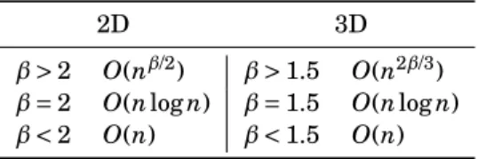
Table 2.1: Flop and storage complexities of the factorization of a sparse system of n = N × N (2D case) or n = N × N × N (3D case) unknowns, assuming a dense factorization complexity O(mβ).
2D 3D
β > 2 O(nβ/2) β > 1.5 O(n2β/3) β = 2 O(n log n) β = 1.5 O(n log n)
β < 2 O(n) β < 1.5 O(n)
Table 2.2: Flop and storage complexities of the FR, BLR, andH factorizations of a sparse system of n = N × N (2D case) or n = N × N × N (3D case) unknowns, derived from the complexities of the factorization of a dense matrix of order m and with a rank bound r. The BLR variant considered is CUFS.
Fds(m, r) Fsp(n, r) Sds(m, r) Ssp(n, r)
2D 3D 2D 3D
FR O(m3) O(n3/2) O(n2) O(m2) O(n log n) O(n4/3)
BLR O(m2r) O(n max(r, log n)) O(n4/3r) O(m3/2r1/2) O(n) O(n max(r1/2, log n)) H O(mr2log2m) O(max(n, n1/2r2)) O(max(n, n2/3r2)) O(mr log m) O(n) O(max(n, n2/3r))
equal to Fsp(N) = L X `=0 (2d)`Fds((N 2`) d−1), (2.4)
where Fds(m) is the dense flop complexity. In BLR, it is given by (2.3). Similarly, the storage complexitySsp(N) is equal to Ssp(N) = L X `=0 (2d)`Sds((N 2`) d−1), (2.5)
whereSds(m) is the dense storage complexity. In BLR, it is given by (2.2).
Assuming a dense complexity O(mβ), it can easily be shown from (2.4) and (2.5) that the sparse complexities only depend on the dense complexity exponentβ and the dimension d. This correspon-dence is reported in Table2.1. The key observation is that a linear O(m) dense complexity is not required to achieve a linearO(n) sparse complexity. In fact, a dense complexity lower than O(m2) and O(m1.5) suffices for 2D and 3D problems, respectively.
Then, the sparse complexities are reported in Table2.2, for the FR, BLR, andH factorizations. Thanks to the key observation above, the BLR sparse complexities are not that far from theH complexities. For example, the BLR 2D storage complexity is already optimal; furthermore, the 2D flop and 3D storage complexities are nearly linear, with only an additional factor depending only on r and log n compared withH . More importantly, thanks to the same key observation, we only need a modest improvement of the dense complexity to reach O(n) complexity. Specifically:
• To drop the max(r, log n) factor in the 2D flop complexity, the dense complexity Fds(m) only
needs to be strictly inferior to O(m2);
• Similarly, to drop the max(r1/2, log n) factor in the 3D storage complexity, the dense com-plexitySds(m) only needs to be strictly inferior to O(m1.5);
• Finally, the superlinear 3D flop complexity can be made linear with a dense complexity Fds(m) strictly inferior to O(m1.5).
The main motivation behind the MBLR format is to find a simple modification of the BLR fac-torization that preserves its simplicity and flexibility, while improving the complexity just enough to get the desired exponent. We will prove in Section5that this complexity improvement can be controlled by the number of levels.
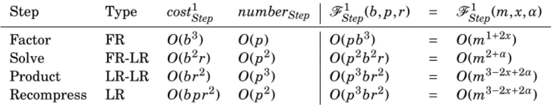
Table 2.3: Main operations for the BLR factorization of a dense matrix of order m, with blocks of size b, and low-rank blocks of rank at most r. We note p = m/b. Type: type of the block(s) on which the operation is performed. cost1Step: cost of performing the operation once. numberStep: number
of times the operation is performed. FStep1 : obtained by multiplying the cost1Stepand numberStep
columns (equation (2.11)). The first expression is given as a function of b, p, and r, while the second is obtained with the assumption that b = O(mx) (and thus p = O(m1−x)) and r = O(mα), for x,α ∈ [0,1].
Step Type cost1Step numberStep FStep1 (b, p, r) = FStep1 (m, x,α)
Factor FR O(b3) O(p) O(pb3) = O(m1+2x)
Solve FR-LR O(b2r) O(p2) O(p2b2r) = O(m2+α)
Product LR-LR O(br2) O(p3) O(p3br2) = O(m3−2x+2α)
Recompress LR O(b pr2) O(p2) O(p3br2) = O(m3−2x+2α)
2.4. Complexity analysis for BLR. To motivate the key idea behind MBLR, let us
sum-marize the dense storage and flop complexity analysis found in [4] that leads to the formulas (2.2) and (2.3). We consider the CUFS variant of the BLR factorization. As indicated in the introduction, we first consider the weakly-admissible case: we assume that all off-diagonal blocks are low-rank. The extension to the strongly-admissible case is provided in the appendix.
We consider a dense BLR matrix of order m. We note b the block size and p = m/b the number of blocks per row and/or column. The amount of storage required to store the factors of such a matrix can be computed as the sum of the storage for the full-rank diagonal blocks and that for the low-rank off-diagonal blocks:
S1
ds(b, p, r) = O(pb
2) + O(p2br). (2.6)
Then, we assume that the block size b is of order O(mx), where x is a real value in [0, 1], and thus the number of blocks p per row and/or column is of order O(m1−x). We also assume that the rank bound is of the form r = O(mα). By replacing b, p, and r by their expression in (2.6), we obtain an expression ofS1
dswhich depends on (m, x,α) instead of (b, p, r):
S1
ds(m, x,α) = O(m1+x) + O(m2−x+α). (2.7)
We then define x∗as the optimal choice of x which minimizes the asymptotic complexity of (2.7).
x∗can be computed as the value which makes each term in (2.7) asymptotically equal. We obtain
x∗= (1 + α)/2, (2.8)
which means the optimal choice of block size is
b∗= O(pmr). (2.9)
This leads to the final dense complexity (already given in (2.2)) S1
ds(m, r) = O(m
1.5pr). (2.10)
Next, to compute the flop complexity, we compute the cost of the Factor, Solve, Product, and Recompress steps and report them in Table2.3(third column). This cost depends on the type (full-rank or low-(full-rank) of the block(s) on which the operation is performed (second column). Note that the Product operation can only take the form of a product of two low-rank blocks (LR-LR), because it involves only off-diagonal blocks, which are low-rank in the weakly-admissible case. We also recall that we have assumed that the matrix is already available in compressed form and thus we do not report the Compress step in Table2.3.
In the weakly-admissible case, there is only one full-rank block on each block-row (the diagonal one); therefore, we can easily count the number of blocks on which each step is performed; we report
(a) Monolevel BLR partitioning. (b) Two-level BLR partitioning. (c) HODLR partitioning Fig. 2.1: Comparison of BLR, MBLR, and hierarchical formats in the weakly-admissible case.
it on the fourth column of Table2.3. The BLR factorization cost of each step is then equal to F1
Step= cost 1
Step× numberStep (2.11)
and is reported in the fifth and sixth columns of Table2.3. In the fifth column, its expression depends on b, p, and r, while in the sixth column it is given as a function of m, x, andα by by substituting b, p, and r by O(mx), O(m1−x), and O(mα), respectively.
The total flop complexity of the dense BLR factorization is equal to the sum of the cost of all steps
F1
ds(m, x,α) = O(m1+2x+ m2+α+ m3−2x+2α). (2.12)
We compute x∗, the optimal choice of x which minimizes the complexity, and find again x∗= (1 + α)/2, which means that the same x∗ value minimizes both the storage and flop complexities, a
valuable property. We finally obtain F1
ds(m, r) = O(m2r). (2.13)
2.5. Key idea of the MBLR format. Let us now consider each step of Table2.3with the objective of reducing the total cost of the factorization. The Product and Recompress steps involve exclusively low-rank blocks and their cost is already optimal as it is linear with respect to the block size b. Therefore, we focus on the Factor and Solve steps. These steps have superlinear cost with respect to b because they involve the diagonal full-rank blocks.
Thus, the key idea of the MBLR format is to further refine these full-rank diagonal blocks by replacing them by BLR matrices. This is illustrated in Figure2.1b. Compared with the BLR format (Figure2.1a), we will show in Section4that this more compressed representation decreases the cost of performing the Factor and Solve steps, which allows to increase the block size to achieve a lower complexity. However, it also remains very different from a hierarchical format (Figure2.1c). First, the diagonal blocks are represented by the simple BLR format, rather than a more complex hierarchical format. Second, while larger than in the BLR case, the off-diagonal blocks are in general still much smaller than in theH case. This has several advantages:
• No relative order is needed between blocks; this allows the clustering to easily be computed and delivers a great flexibility to distribute the data in a parallel environment.
• The size of the blocks can be small enough to fit on a single shared-memory node; there-fore, in a parallel environment, each processor can efficiently and concurrently work on different blocks.
• To perform numerical pivoting, the quality of the pivot candidates in the off-diagonal blocks Fik can be estimated with the entries of its low-rank basis Yik, provided that Xik
is an orthonormal matrix. However, as explained in [25], the quality of this estimation depends on the size of the block; smaller blocks lead to a tighter estimate. This makes the BLR format particularly suitable to handle numerical pivoting, a critical feature lacking in most hierarchical solvers presented in the literature.
I I1 I2
I3 I4 I5 I6
I7 I8 I9 I10 I11 I12 I13 I14 (a) Cluster tree.
I I1 I2 I3 I4 I5 I6 I7 I8 I9 I10 I11 I12 I13 I14 (b) HODLR block-clustering.
Fig. 3.1: An example of cluster tree and its associated HODLR block-clustering.
While many advantages of the BLR and MBLR formats lie in their efficiency and flexibility in the context of a parallel execution, the parallel implementation of the MBLR format is out of the scope of this paper. Similarly, we omit a detailed description of the algorithms designed to handle numerical pivoting; see [25] for a thorough discussion. In this paper, we focus on the theoretical complexity analysis of the MBLR factorization.
3. Difference between MBLR and H matrices. In this section, we first explain how
MBLR matrices can be represented using the cluster tree modelization typically used in theH literature; this provides a convenient tool to formalize the key difference between the MBLR and hierarchical formats that was informally presented in the previous section: the number of levels in the cluster tree is a constant in the MBLR format, while it is logarithmically dependent on the problem size in theH format.
Using this formalism,H theory is thus applicable to the MBLR format; however, we show in Section3.3that it leads to very pessimistic complexity bounds. We must therefore develop a new theory to compute satisfying bounds, which is the object of Sections4and5. Since the proofs and computations in these sections are not based on theH theory, this section may be skipped by the reader, at least on a first read.
3.1. The hierarchical case. Here, we briefly recall the definition of cluster trees, and how
they are used to represent hierarchical partitionings. We refer to [10,22] for a formal and detailed presentation.
Let us noteI the set of unknowns. We assume that the sets of row and column indices of the matrix are the same, for the sake of simplicity, and because we do not need to distinguish them for the purpose of this section.
Computing a recursive partitionS(I ) of I can be modeled with a so-called cluster tree. DEFINITION3.1 (Cluster tree). LetI be a set of unknowns and TI a tree whose nodesv are associated with subsetsσvofI . TI is said to be a cluster tree iff:
• The root of TI, notedr, is associated withσr= I ;
• For each non-leaf node v ∈ TI, with children notedCTI(v), the subsets associated with the
children form a partition ofσv, that is, theσcsubsets are disjoint and satisfy
[
c∈CTI(v)
σc= σv.
An example of cluster tree is provided in Figure3.1a. As illustrated, cluster trees establish a hierarchy between clusters. A given cluster tree uniquely defines a weakly-admissible, hierarchical block-clustering (so-called HODLR matrix), as illustrated in Figure3.1b.
Note that the cluster tree is not enough to define general, strongly-admissible hierarchical block-clusterings such as an H block-clustering. In that case, a new tree structure, so-called block-cluster tree, must be introduced. For the sake of simplicity, we do not discuss them here, since cluster trees (and weakly-admissible hierarchical block-clusterings) are enough to explain the difference between MBLR and hierarchical matrices.
I
I1 I2 I3 I4 I5
(a) Flat cluster tree.
I I1 I2 I3 I4 I5 (b) BLR block-clustering.
Fig. 3.2: An example of flat cluster tree and its associated BLR block-clustering.
I
I1 I2 I3
I4 I5 I6 I7 I8 I9 I10I11I12
(a) Cluster tree of depth 2.
I I1 I2 I3 I4 I5 I6 I7 I8 I9 I10 I11 I12 (b) Two-level BLR block-clustering.
Fig. 3.3: An example of cluster tree of depth 2 and its associated two-level BLR block-clustering.
3.2. The BLR and MBLR formats, explained with cluster trees. It is interesting to first
mention how the BLR format can be viewed as a very particular kind ofH -matrix. In [4], we made a first attempt to model BLR partitionings with cluster trees, where the BLR partitioning is defined using only the leaves of the cluster tree. However, this model is inadequate because the other nodes of the tree are unnecessary (and thus there are several possible cluster trees for a unique BLR partitioning).
Therefore, we newly propose to define a given BLR partitioning with a unique, flat cluster tree of depth 1, as illustrated in Figure3.2.
With this definition, it is straightforward to extend the model to the MBLR format. An `-level BLR block-clustering can be represented by a cluster tree of depth`. This is illustrated in Figure3.3in the two-level case.
It is thus clear that, just like the BLR format, the MBLR one can also be viewed as a very particular kind ofH -matrix, since any MBLR matrix can be represented with a cluster tree that satisfies Definition3.1. However, whileH -matrices are indeed also represented by cluster trees, in practice, they are virtually always built with an implicit assumption: the number of children of any node in the cluster tree is constant with respect to the size of the matrix. Most commonly, cluster trees are binary trees, and thus this number is 2. Since the diagonal blocks of anH -matrix are of constant size, this leads to O(log m) levels in the cluster tree.
The MBLR format is based on the converse approach: the number of levels is fixed to some constant` = O(1), which in turn leads to a number of children per node that is asymptotically dependent on m. For example, assuming a constant rank r = O(1), we will prove in Section4that a two-level BLR matrix is represented by a cluster tree with O(m1/3) nodes on the first level (children of the root node), and each of these nodes has O((m2/3)1/2) = O(m1/3) children on the second level.
While this is technically not prohibited by the generalH -format definition, it has, to the best of our knowledge, never been considered in theH literature. As a matter of fact, in his recent book, Hackbusch writes ([22], p.83): ‘The partition should contain as few blocks as possible since the storage cost increases with the number of blocks”. While that is true, we believe that the smaller size and greater number of blocks can provide a gain in flexibility that can be useful in a
parallel solver.
One may in fact find it surprising that this simple idea of having a constant number of levels has never been proposed before. We believe that this is mainly explained by the fact that the H theoretical formalism does not provide a satisfying result if applied to the MBLR format, as explained in the following.
3.3. H theory leads to pessimistic MBLR complexity bounds. In [4, Section 3.2], we explained that applying theH theoretical complexity formulas to the BLR format does not provide a satisfying complexity bound. Here, we show this remains the case for the MBLR format.
The storage and flop complexities of the factorization of a denseH -matrix of order m have been shown [20] to be
SdsH(m) = O(mLcspmax(rmax, bdiag)), (3.1)
FdsH(m) = O(mL 2c2
spmax(rmax, bdiag)2). (3.2)
L is the depth of the cluster tree. cspis the so-called sparsity constant, defined as the maximum
number of blocks of a given level in the cluster tree that are in the same row or column of the matrix; it is a measure of how much the original matrix has been refined. rmax is the maximal
rank of all the blocks of the matrix, while bdiag is the size of the diagonal blocks. Note that the
power to which cspis elevated to in the flop complexity depends on the reference considered. The
term c3spis found in [20]; a reduced complexity with c2spinstead is given in [11]. Since our aim is to show that theH complexity formulas do not provide a satisfying result when applied to MBLR matrices, in the following, we use the best case formula with c2sp; the formula with c3spwould lead to an even more pessimistic complexity bound.
Under some assumptions on how the partition S(I ) is built [20, Lemma 4.5], the sparsity constant can be bounded by O(1) in theH case. By recursively refining the diagonal blocks until they become of constant size, we have bdiag= O(1) and L = O(log m). Therefore, (3.1) and (3.2) lead
toSH
ds (m) = O(rm log m) and FdsH(m) = O(r
2m log2m).
In the BLR case, we have L = 1 and bdiag= b; the sparsity constant is equal to the number of
blocks per row m/b, a high value that translates the fact that BLR matrices are much more refined than hierarchical ones. This leads toSdsH ,1(m) = O(m2) andFdsH ,1(m) = O(m3), where the notation SdsH ,1 andFH ,1
ds signifies “H complexity formula applied to the monolevel BLR case”. We thus
obtain a very pessimistic complexity bound, which is due to the fact that the diagonal blocks are of the same size as all the other blocks, i.e., bdiag= b.
Applying the formulas to the MBLR case leads to the same problem. Assuming that r = O(1) for the sake of simplicity, let us consider the two-level case and denote by b1and b2the outer and
inner blocks sizes, respectively. We have L = 2, bdiag= b2, and csp= max(m/b1, b1/b2). The storage
complexity
SdsH ,2(m) = O(max(m2b2/b1, mb1))
is minimized for b1= O(pm) and b2= O(1), and equal to O(m3/2), which is not a satisfying result
since we have proven in Section2.4that this is the BLR complexity. A similarly unsatisfying result is obtained for the flop complexity, again minimized for b1= O(pm) and b2= O(1) and equal to
FdsH ,2(m) = O(max(m3b22/b21, mb21)) = O(m2).
Does the problem persist with a higher number of levels`? The answer is unfortunately positive. Indeed, we have
SdsH ,`(m) = O( max
i=0,`−1(
mbib`
bi+1 )),
with the notation b0= m. To minimize the expression, we equilibrate each term in the maximum,
which leads to the recursive relation b2i= bi−1bi+1. Noting b1= b the outer block size, it is clear
that the closed-form expression of biis bi= bi/mi−1. Since the smallest block size blmust be at
least O(1), this leads to
b`
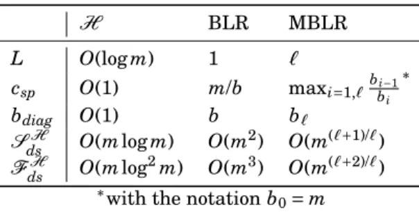
Table 3.1: Applying theH theoretical complexity formulas to the BLR or MBLR cases does not provide a satisfying result. We have assumed that r = O(1) for the sake of clarity, but the bounds would remain pessimistic for general ranks.
H BLR MBLR
L O(log m) 1 `
csp O(1) m/b maxi=1,`bbi−1i
∗
bdiag O(1) b b`
SdsH O(m log m) O(m
2) O(m(`+1)/`)
FH
ds O(m log
2m) O(m3) O(m(`+2)/`)
∗with the notation b 0= m
and thus b ≥ O(m(`−1)/`), which in turn leads to the complexity bound
SdsH ,`(m) ≥ O(m
2b
`
b1 ) ≥ O(m (`+1)/`).
In Section5, we will prove that for r = O(1) we have Sds`(m) = O(m(`+2)/(`+1)), which is a better bound, especially when considering a small number of levels`. The analysis for the flop complexity leads to the same expression of biand to the complexity boundFdsH ,`(m) = O(m(`+2)/`), which is
again overly pessimistic compared with the boundFds`(m) = O(m(`+3)/(`+1)) that we will prove in Section5.
We summarize the result of applying theH complexity formulas in Table3.1. It is interesting to note that these bounds overestimate the actual complexity by exactly one level. This is actually not surprising: in theH theory, all the blocks at the bottom level are assumed to be non-admissible, which accounts for the “loss” of one level in the complexity bounds.
It is therefore clear that we must develop a new theory extending theH formalism to be able to prove better MBLR complexity bounds, just as we did in [4] for the BLR case. We begin by the two-level case in the next section.
4. Two-level BLR matrices. In this section, we compute the theoretical complexity of the
two-level BLR factorization. The proofs and computations on this particular two-level case are meant to be illustrative of those of the general multilevel case with an arbitrary number of levels, which is discussed in Section5.
We remind the reader that in this section, we are considering the weakly-admissible case only.
4.1. Two-level kernels description. In order to adapt Algorithm2.1to two-level BLR ma-trices, two modifications must be performed.
First, the Factor kernel is not a full-rank factorization of the diagonal blocks Fkkanymore, but
a BLR factorization. Thus, line14must be replaced by e
Fkk= eLkkUekk=BLR-Factor(Fkk) , (4.1)
whereBLR-Factorrefers to the BLR factorization described in Algorithm2.1.
Second, the FR-LR Solve kernel at lines16and17must be changed to a BLR-LR Solve: e Fik←BLR-LR-Solve¡Uekk,Feik¢ (4.2) e Fki←BLR-LR-Solve ¡ e Lkk,Feki¢ , (4.3)
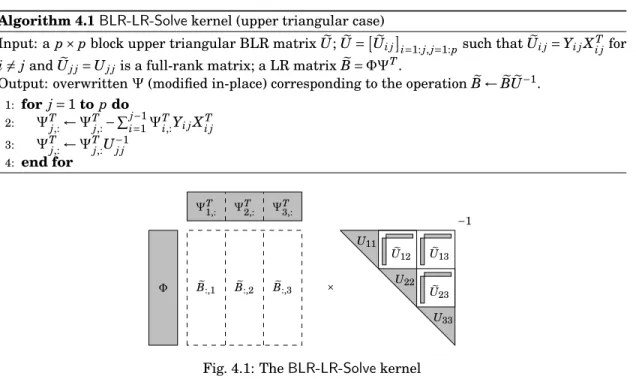
whereFeikandFekiare LR matrices andLekkandUekkare lower and upper triangular BLR matrices. We describe in Algorithm4.1theBLR-LR-Solve kernel, in the upper triangular case, omitting the lower triangular case which is very similar. The kernel consists in applying a triangular solve with a upper triangular BLR matrixU to a low-rank matrixe B =e ΦΨT. We recall thatUei jdenotes
Algorithm 4.1BLR-LR-Solvekernel (upper triangular case) Input: a p × p block upper triangular BLR matrix eU;U =e
£ e
Ui j¤i=1: j, j=1:psuch thatUei j= Yi jXTi jfor
i 6= j and eUj j= Uj jis a full-rank matrix; a LR matrixB =e ΦΨT.
Output: overwrittenΨ(modified in-place) corresponding to the operationB ← ee BUe−1. 1: for j = 1 to p do 2: ΨT j,:←Ψ T j,:− Pj−1 i=1Ψ T i,:Yi jX T i j 3: ΨT j,:←Ψ T j,:U−1j j 4: end for Φ ΨT 1,: ΨT2,: ΨT3,: e B:,1 Be:,2 Be:,3 × U11 U22 U33 −1 e U12 Ue13 e U23
Fig. 4.1: TheBLR-LR-Solvekernel
the (i, j)-th low-rank sub-block ofU (with the notatione Uej j= Uj j), and thatΨj,:denotes the j-th
block-row ofΨ.
Two main operations must be performed: a triangular solve using the full-rank diagonal blocks Uj jofU, and an update using the low-rank off-diagonal blockse Uei j= Yi jXi jT ofU. Both are appliede on the low-rank block-columnsBe:, j=ΦΨTj,:ofB. These two operations take place at linese 3and2 of Algorithm4.1, respectively.
The FR-LR triangular solve can be written as
e B:, j← eB:, jU−1j j =Φ ³ ΨT j,:U−1j j ´ (4.4) and thus onlyΨTj,:needs to be updated, as shown at line3.
The LR-LR update takes the following form:
e
B:, j← eB:, j−Pj−1i=1Be:,iUei j =ΦΨTj,:−Pj−1i=1Φ
³ ΨT i,:Yi jXTi j ´ =Φ ³ ΨT j,:− Pj−1 i=1Ψ T i,:Yi jX T i j ´ (4.5)
and thus, again, onlyΨTj,:needs to be updated, as shown at line2. TheBLR-LR-Solvekernel is illustrated in Figure4.1.
It can easily be computed that the cost of applying theBLR-LR-Solvekernel once is equal to the storage complexity times the rank bound r:
cost2Solve= O(r) × Sds1(b, r). (4.6) Injecting (2.10) into (4.6) leads to
cost2Solve= O(b3/2r3/2). (4.7)
4.2. Two-level complexity analysis. We now compute the complexity of the two-level BLR
factorization of a dense matrix F of order m. We reuse the monolevel notations for the top level. We denote by b the size of the first-level blocks and p = m/b the number of of rows and block-columns. We assume that b is of the form b = mx, for x ∈ [0,1]. We also assume that the ranks of the off-diagonal blocks are bounded by r = O(mα).
Table 4.1: Two-level equivalent of Table2.3. The legend of the table is the same. The differences between the two tables are highlighted in gray.
Step Type cost2Step numberStep FStep2 (b, p, r) = FStep2 (m, x,α)
Factor BLR O(b2r) O(p) O(pb2r) = O(m1+x+α)
Solve BLR-LR O(b3/2r3/2) O(p2) O(p2b3/2r3/2) = O(m2−x/2+3α/2)
Product LR-LR O(br2) O(p3) O(p3br2) = O(m3−2x+2α)
Recompress LR O(b pr2) O(p2) O(p3br2) = O(m3−2x+2α)
The size required to store the factors is again the sum of the storage for the diagonal and off-diagonal blocks, as in (2.6). The difference is that the off-diagonal blocks are not full-rank but BLR matrices. They are further refined into smaller blocks whose size should be chosen of order O(pbr), as determined by (2.9) in the BLR complexity analysis. Therefore, in the two-level case, (2.6) becomes S2 ds(b, p, r) = p × S 1 ds(b, r) + O(p 2br). (4.8)
By replacingSds1(b, r) by its second expression computed in (2.10), we obtain S2
ds(b, p, r) = O(pb 3/2r1/2
) + O(p2br) (4.9)
Finally, we replace b, p, and r by their expression O(mx), O(m1−x), and O(mα), respectively, to obtain
S2
ds(m, x,α) = O(m1+(x+α)/2+ m2−x+α). (4.10)
This leads to
x∗= (2 + α)/3, (4.11)
where x∗defines the optimal choice of the first-level block size b. We thus obtain a final two-level
storage complexity of
S2
ds(m, r) = O(m
4/3r2/3). (4.12)
We now compute the flop complexityFds2(m, r) of the two-level BLR dense factorization. We compute the cost of each step and report it in Table4.1, which is the two-level equivalent of Ta-ble2.3; the differences between the two tables are highlighted in gray. The Product and Recom-press steps have not changed and thus have the same cost. The Factor step consists in factorizing the p diagonal blocks which are now represented by BLR matrices; thus its cost is directly derived from the BLR complexity computed in (2.13):
F2
Factor(b, p, r) = p × F 1
ds(b, r) = O(pb
2r). (4.13)
It remains to compute the cost of the Solve step, which now takes the form of O(p2) calls to the
BLR-LR-Solvekernel whose cost is given by (4.7). Thus, the overall cost of the Solve step is F2
Solve(b, p, r) = O(p
2b3/2r3/2). (4.14)
This concludes the computations for the third, fourth, and fifth columns of Table4.1. Just as in the monolevel case, the sixth column is obtained by replacing b, p, and r by their expression O(mx), O(m1−x), and O(mα), respectively.
We can finally compute the total flop complexity as the sum of the costs of all steps F2
ds(m, x,α) = O(m1+x+α+ m2−x/2+3α/2+ m3−2x+2α) (4.15)
We then compute x∗which is again equal to the same value as the one that minimizes the storage
complexity, x∗= (2 + α)/3. Therefore, the final two-level dense flop complexity is
F2
ds(m, r) = O(m
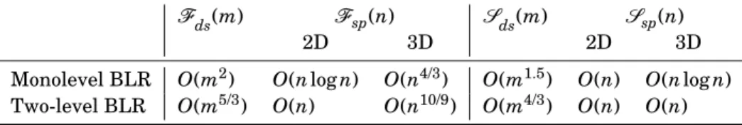
Table 4.2: Flop and storage complexities of the monolevel and two-level BLR factorizations of a sparse system of n = N × N (2D case) or n = N × N × N (3D case) unknowns, derived from the complexities of the factorization of a dense matrix of order m. We consider a constant rank bound r = O(1). The BLR variant considered is CUFS.
Fds(m) Fsp(n) Sds(m) Ssp(n)
2D 3D 2D 3D
Monolevel BLR O(m2) O(n log n) O(n4/3) O(m1.5) O(n) O(n log n) Two-level BLR O(m5/3) O(n) O(n10/9) O(m4/3) O(n) O(n)
The two-level BLR format therefore significantly improves the asymptotic storage and flop complexity compared with the monolevel format. Our analysis shows that the top level block size should be set to b∗= O(mx∗) = O(m2/3r1/3). This is an asymptotically larger value than the
monolevel optimal block size computed in (2.9), which translates the fact that by refining the diag-onal blocks, we can afford to take a larger block size to improve the overall asymptotic complexity. However, contrarily to hierarchical matrices, b∗ remains asymptotically much lower than O(m);
this makes the format much more flexible for the reasons described in Section2.5. In short, we have traded off some of the flexibility of the monolevel format to improve the asymptotic complexity. This improvement of the dense flop and storage complexities is translated into an improvement of the sparse complexities. Assuming a rank bound in O(1), we quantify this improvement in Table4.2. Compared with the monolevel BLR format, the two-level BLR format drops the O(log n) factor in the 2D flop and 3D storage complexities, which become linear and thus optimal. The two-level BLR format can thus achieve, in these two cases, the same O(n) complexity as the hierarchical formats while being almost as simple and flexible as flat formats.
Finally, the 3D flop complexity remains superlinear but is significantly reduced, from O(n4/3) to O(n10/9). As the problem size gets larger and larger, even small asymptotic improvements can make a big difference. Therefore, we now generalize the two-level analysis to the multilevel case with an arbitrary number of levels.
5. Generalization to`-level BLR matrices. In this section, we generalize two-level proof
and computations of the previous section to an arbitrary number of levels` by computing recursive complexity formulas. We remind the reader that in this section, we are still considering the weakly-admissible case only.
5.1. Recursive complexity analysis. Just as for the two-level case, one can compute the
three-level asymptotic complexities, and so on until the general formula becomes clear. We state the result for an arbitrary number of levels` in the following theorem. Note that it is important to assume that the number of levels` is constant (` = O(1)), since the constants hidden in the big O depend on`.
THEOREM5.1 (Storage and flop complexity of the`-level BLR factorization). Let us consider a dense`-level BLR matrix of order m. We note b the size of the top level blocks, and p = m/b. Let r = O(mα) be the bound on the maximal rank of any block on any level. Then, the optimal choice of the top level block size isb = O(mx∗), with x∗= (` + α)/(` + 1), which leads to the following storage
and flop complexities:
Sds`(m, r) = O(m
(`+2)/(`+1)r`/(`+1)); (5.1)
F`
ds(m, r) = O(m
(`+3)/(`+1)r2`/(`+1)). (5.2)
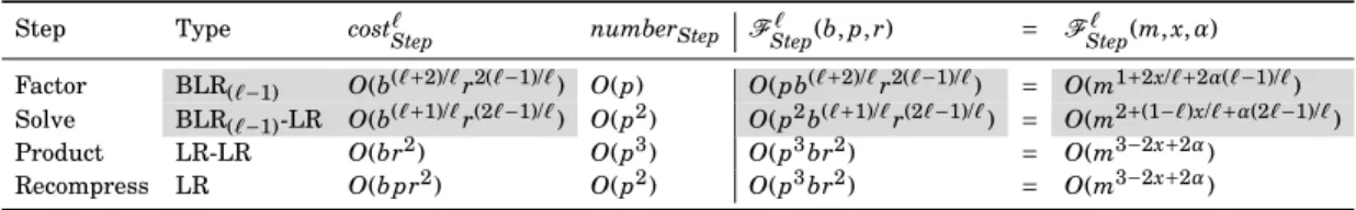
Table 5.1: `-level equivalent of Tables 2.3 and 4.1. The legend of the table is the same. The differences between this table and the previous two are highlighted in gray.
Step Type cost`
Step numberStep FStep` (b, p, r) = FStep` (m, x,α)
Factor BLR(`−1) O(b(`+2)/`r2(`−1)/`) O(p) O(pb(`+2)/`r2(`−1)/`) = O(m1+2x/`+2α(`−1)/`) Solve BLR(`−1)-LR O(b(`+1)/`r(2`−1)/`) O(p2) O(p2b(`+1)/`r(2`−1)/`) = O(m2+(1−`)x/`+α(2`−1)/`)
Product LR-LR O(br2) O(p3) O(p3br2) = O(m3−2x+2α)
Recompress LR O(b pr2) O(p2) O(p3br2) = O(m3−2x+2α)
check their asymptotic dependence on`. We therefore seek to prove the recursive bounds Sds`(m, r) ≤ C`m
(`+2)/(`+1)r`/(`+1),
Fds`(m, r) ≤ C0`m(`+3)/(`+1)r2`/(`+1),
where C`and C0
` are constants independent of m. The formulas hold for` = 1 with C1= 2 and
C01= 4. Let us assume that they are true for the (` − 1)-level BLR factorization and prove that they still hold for the`-level one.
S`
ds(m, r) can be computed as the storage cost for the off-diagonal low-rank blocks (whose
num-ber is less than p2) plus that of the p diagonal blocks, which are represented as (` − 1)-level BLR matrices. Therefore, by induction,
Sds`(b, p, r) ≤ p × Sds`−1(b, r) + p 2
br ≤ pC`−1b(`+1)/`r(`−1)/`+ p2br. We replace b, p, and r by their expression mx, m1−x, and mα, respectively, to obtain
Sds`(m, x,α) ≤ C`−1m1−x+(`+1)x/`+α(`−1)/`+ m2−x+α. For x∗= (` + α)/(` + 1), we obtain S` ds(m,α) ≤ C`−1m (`+2+α`)/(`+1)+ m(`+2+α`)/(`+1) and therefore Sds`(m, r) ≤ C`m (`+2)/(`+1)r`/(`+1),
with C`= C`−1+ 1 (and thus C`= ` + 1).
We now consider the flop complexity. Fds`(m, r) can be computed as the sum of the costs of the Factor, Solve, Product and Recompress steps. We provide the`-level equivalent of Tables2.3 and4.1in Table5.1. The Product and Recompress steps do not depend on` and their cost is less than p3br2≤ m3−2x+2α. The Solve step consists in applying less than p2 times theBLR(`−1)
-LR-Solvekernel, described in Algorithm5.1, where BLR(`−1)denotes a (` − 1)-level BLR matrix (with
the convention that BLR0denotes a FR matrix). It can easily be proven by induction that the cost
of applying theBLR(`−1)-LR-Solvekernel is less than r × Sds`−1(b, r). Therefore, it holds
FSolve` (p, b, r) ≤ p 2 r × Sds`−1(b, r) ≤ C`−1p 2b(`+1)/`r(2`−1)/`, and thus FSolve` (m,α, x) ≤ C`−1m2+(1−`)x/`+α(2`−1)/`.
The Factor step consists in factorizing p diagonal (` − 1)-level BLR matrices and therefore, by induction,
FFactor` (p, b, r) ≤ pC0`−1b(`+2)/`r2(`−1)/`≤ C0`−1m1+2x/`+2α(`−1)/`.
Summing the cost of all steps yields
2 4 6 8 10 1 1.1 1.2 1.3 1.4 1.5 1.6 1.7 1.8
(a) Storage complexity.
2 4 6 8 10 1 1.2 1.4 1.6 1.8 2 2.2 2.4 2.6 (b) Flop complexity.
Fig. 5.1: Theoretical asymptotic exponent of the storage and flop complexity of the dense MBLR factorization Taking x∗= (` + α)/(` + 1), we obtain F` ds(m,α) ≤ (C0`−1+ C`−1+ 2)m (`+3+2α`)/(`+1) and thus Fds`(m, r) ≤ C0`m(`+3)/(`+1)r2`/(`+1),
with C0`= C0`−1+ C`−1+ 2 (and thus C0`= `(` + 1)/2 + ` + 2). Since the number of levels ` is assumed to be constant, we have C`= O(C0
`) = O(1) which concludes the proof.
Algorithm 5.1BLR`-LR-Solvekernel,` > 1 (upper triangular case)
Input: a p × p block upper triangular BLR`matrixU;e U =e £
e Ui j
¤
i=1: j, j=1:psuch thatUei j= Yi jXi jT for
i 6= j and eUj jis a BLR(`−1)matrix; a LR matrixB =e ΦΨT.
Output: overwrittenΨ(modified in-place) corresponding to the operationB ← ee BUe−1. 1: for j = 1 to p do 2: ΨTj,:←ΨTj,:−Pj−1 i=1Ψ T i,:Yi jXi jT 3: BLR(`−1)-LR-Solve ³ e Uj j,ΦΨTj,: ´ 4: end for
5.2. Influence of the number of levels`. With the formulas from Theorem5.1proven, we now analyze their practical implications. It is clear that both the storage and flop asymptotic com-plexities decrease monotonically with the number of levels, while the top level block size increases. In Figure5.1, we plot the value of the exponent of the asymptotic complexities as a function of the number of levels, for different rank bounds r = O(mα).
Let us first consider the case of r = O(1) (i.e., α = 0). We have already shown that, in this case, the two-level BLR factorization has O(m5/3) flop complexity, which leads to O(n10/9) 3D sparse complexity. With a third level, the dense complexity decreases to O(m3/2), which is precisely the 3D sparse breaking point (see Table2.1), and thus leads to O(n log n) complexity. The log factor can be dropped by adding a fourth level. The dense complexity tends towards O(m) as the number of levels increases, but the sparse complexity cannot be further improved after the optimal O(n) has been reached. This illustrates that only a small number of levels is necessary to reach low sparse complexity. In particular, with four levels, the number of blocks on the top level is p = O(m1/5),
which is still a quite large number which, as previously described, provides more flexibility to address issues such as data distribution, parallel implementation, numerical pivoting, etc.
The picture is different with higher rank bounds. Indeed, the higher the rank, the more diffi-cult it is to reach a low complexity and thus more levels are required. For example, with r = O(pm) (α = 1/2), it is actually not possible to reach a O(n) 3D flop complexity since the dense complexity is at best O(mr2) = O(m2). This is the dense complexity achieved by the hierarchical formats, as well as the MBLR format with an infinite number of levels, and leads to O(n4/3) sparse complexity. It is therefore not possible to achieve this complexity with a constant number of levels. However, a cru-cial observation is that the rate of improvement of the exponent, which follows (` +3+2α`)/(`+1), is rapidly decreasing as` increases. For example, with α = 1/2, one level decreases the full-rank O(m3) complexity to the BLR O(m2.5) complexity; it would require an infinite number of levels to achieve another O(m0.5) factor of gain. Similarly, adding two more levels leads to O(m2.25), achiev-ing a O(m0.25) gain which can only be achieved again with infinitely more levels! This illustrates the critical observation that the first few levels achieve most of the asymptotic gain. We therefore believe that the MBLR factorization with only a small number of levels can be of practical interest, even for problems with larger ranks.
5.3. Comparison with the BLR-H format. We conclude this section by comparing our
MBLR format to the related BLR-H format, sometimes also referred to as “Lattice-H ”. It consists in representing the matrix using the BLR format, and then approximating its diagonal blocks with H -matrices. The BLR-H format has been considered as a simple way to use hierarchical matrices in a distributed-memory setting [23,1] but has been little studied from a theoretical standpoint. The question is whether refining the diagonal blocks with additional levels (as H rather than MBLR matrices) improves the asymptotic complexity of the format. In the following, we prove that this is not the case and therefore recommend the use of the MBLR format over that of the BLR-H one.
The complexity of the BLR-H format is entirely determined by the block size b used for the BLR partitioning. Indeed, the storage complexity can be computed as the sum of the storage for the off-diagonal low-rank blocks and that of the diagonalH blocks:
SBLR−H
ds (p, b, r) = O(p 2
br) + O(pbr log b) = O(p2br),
where p = m/b. Thus, the term corresponding to the off-diagonal low-rank blocks is dominant and we obtain
SBLR−H
ds (m, b, r) = O(
m2r
b ). (5.3)
Similarly, the flop complexity of the BLR-H factorization is dominated by the LR-LR-Product and Recompress steps which cost
FBLR−H ds (m, b, r) = O(p 3br2 ) = O(m 3r2 b2 ). (5.4)
Applying (5.3) and (5.4) with the optimal choice of block size for the `-level BLR format, b = O(m`/(`+1)r1/(`+1)), we obtain the same asymptotic complexity as that proved in Section 5 (Theo-rem5.1): SBLR−H ds (m, r) = Sds`(m, r) = O(m (`+2)/(`+1)r`/(`+1)); FBLR−H ds (m, r) = Fds`(m, r) = O(m (`+3)/(`+1)r2`/(`+1)).
This result can be interpreted as follows: for any given block size b, there exists a constant number of levels`b such that representing the diagonal blocks of the matrix as `b-level BLR matrices
suffices to achieve the lowest possible complexity. As far as asymptotic complexity is concerned, it is thus not necessary to represent these diagonal blocks with theH format. Note that the value of `bcan easily be computed as
`b= min
n
6. Numerical experiments. In this section we compare the experimental complexities of the
full-rank, BLR, and MBLR formats (with different numbers of levels) for the factorization of dense matrices arising from Schur complements of sparse problems.
We have developed a MATLAB code to perform the BLR and MBLR factorization of a dense matrix, which we use to run all experiments. The objective of this experimental section is purely to validate the theoretical complexity bounds that we have computed in Theorem5.1. Assessing the practical performance of the MBLR factorization is complex, not our focus in this paper and will be the objective of future work; numerical experiments with sparse matrix factorizations are also out of the scope of this article.
6.1. Experimental setting. All the experiments were performed on the brunch computer
from the LIP laboratory (ENS Lyon), a shared-memory machine equipped with 24 Haswell proces-sors and 1.5 TB of memory.
To validate our theoretical complexity results, we use a Poisson problem, which generates the symmetric positive definite matrix A from a 7-point finite-difference discretization of equation
−∆u = f
on a 3D domain of size n = N × N × N with Dirichlet boundary conditions. We compute the dense MBLR factorization of the matrices F corresponding to the root separator of the nested dissection partitioning, which are of order m = N2.
To compute the low-rank form of the blocks, we perform a truncated QR factorization with column pivoting (i.e., a truncated version of LAPACK’s [8]_geqp3routine). We use a mix of fixed-accuracy and fixed-rank truncation: we stop the factorization after either an fixed-accuracy ofε has been achieved or at most rmaxcolumns have been computed. In the following experiments, we have set ε = 10−14and we compare two choices of r
max, 10 and 40.
Note that in the weakly admissible context, fixing the rank to some constant yields a limited accuracy, measured by either kF − LUk or kI − U−1L−1Fk: in our case, both quantities are of the
order of 10−1, both for r
max= 10 and rmax= 40. Indeed, increasing rmax barely improves the
accuracy because some off-diagonal blocks have almost full numerical rank. While an error of the order of 10−1could be enough to build a preconditioner, achieving a higher accuracy would require
a strongly admissible implementation. The generalization of the MBLR format to the strongly admissible case is therefore of great importance and, while its practical implementation is outside the scope of this article, we provide its algorithmic description in the appendix. We prove that its theoretical complexity is identical to that of the weakly admissible case; we also include some very preliminary experiments showing that its complexity is in agreement with the theory while leading to a much higher accuracy.
6.2. Experimental estimates of the complexity. We first experimentally estimate the
ex-ponents in the asymptotic complexities of the dense MBLR factorization, using a number of levels ` varying from 1 to 4. To do so, we use the least-squares estimation of the coefficients β1,β2of the
regression function Xf it= eβ ∗ 1Nβ∗2 withβ∗ 1,β∗2= argminβ 1,β2k log X obs− β1− β2log Nk2.
such that Xf itfits the observed data Xobs.
We report in Figure6.1the measured storage and flops costs, along with the estimate of the exponent (β1) obtained by the fitting. Figure6.1corresponds to rmax= 40; the results for rmax= 10
(not shown) are similar. In Table6.1we summarize these estimated exponents and compare them to the theoretical ones. The estimated exponents slightly differ from their theoretical counterpart, and may depend on various factors such as the choice of the block sizes, or the actual value of the numerical ranks, but overall these results are in relatively good agreement with the theory. The crucial observation is that, for both choices of rmax, an asymptotic gain is achieved by each addition
of a new level, at least up to` = 4.
We now analyze the sharpness of the constant prefactors in the theoretical bounds (5.1) and (5.2) computed in Theorem5.1. To do so, we report in Figure6.2the ratio between the measured
(a) Storage. (b) Flops.
Fig. 6.1: Experimentally estimated exponents in the asymptotic complexities of the dense MBLR factorization of the root separator (of order m = N2) of a 3D Poisson problem (of order n = N3).
Table 6.1: Comparison between theoretical and experimental complexities.
` = 1 ` = 2 ` = 3 ` = 4
Storage complexity
Theoretical O(m1.50) O(m1.33) O(m1.25) O(m1.20) Experimental (rmax= 10) O(m1.47) O(m1.36) O(m1.32) O(m1.27)
Experimental (rmax= 40) O(m1.37) O(m1.29) O(m1.25) O(m1.24)
Flop complexity
Theoretical O(m2.00) O(m1.67) O(m1.50) O(m1.40)
Experimental (rmax= 10) O(m1.97) O(m1.68) O(m1.62) O(m1.51)
Experimental (rmax= 40) O(m1.92) O(m1.63) O(m1.49) O(m1.41)
(a) Storage. (b) Flops.
Fig. 6.2: Ratio between the measured costs and their theoretical bound for the MBLR factorization of the root separator (of order m = N2) of a 3D Poisson problem (of order n = N3), with rmax= 40.
cost and these bounds in the case rmax= 40; the results for rmax= 10 are again similar. The figure
shows that the bounds are almost sharp: the actual constants are in all cases within an order of magnitude of their bound. While their sharpness seems to decrease as the number of levels` increases (this is especially the case for the storage cost), the important observation is that the ratio remains more or less constant as n increases (flat curves), which means that the asymptotic cost of the MBLR factorization behaves as expected. Note that for` = 1, the storage cost is actually slightly over the bound: this may be explained by a suboptimal choice of block size.
Overall, these experimental results therefore support the capacity of the MBLR format to significantly reduce the asymptotic complexity of the factorization, even when only a small number of levels is used.
7. Conclusion. We have proposed a new multilevel BLR (MBLR) format to bridge the gap
be-tween flat and hierarchical low-rank matrix formats. Contrarily to hierarchical formats for which the number of levels in the block hierarchy is logarithmically dependent on the size of the problem, the MBLR format only uses a constant number of levels`.
We had previously explained why theH -matrix theory, while applicable to the BLR format, leads to very pessimistic complexity bounds and is therefore not suitable. Here, we have shown that this remains true for the MBLR format and we therefore extended the theory to compute bet-ter bounds. We proved that both the storage and flop complexities of the factorization can be finely controlled by`. We theoretically showed that the first few levels achieve most of the asymptotic gain that can be expected. In particular, for a sparse 3D problem with constant ranks, two lev-els suffice to achieve O(n) storage complexity and three levlev-els achieve O(n log n) flop complexity, suggesting that a small number of levels may be enough in practice. Our numerical experiments confirm this trend.
Having a small number of levels leads to a greater freedom to distribute data in parallel; in particular blocks are small enough for several of them to fit in shared-memory, allowing an efficient parallelization. Finally, a small number of levels greatly simplifies the implementation of the format, making it easy to handle important features such as dynamic data structures and numerical pivoting. The related BLR-H (or Lattice-H ) format targets a similar objective; however, our theoretical analysis shows that using more levels to refine the diagonal blocks actually does not improve the asymptotic complexity with respect to the MBLR format.
In short, the MBLR format aims to strike a balance between asymptotic complexity and actual performance on parallel computers by trading off the optimal hierarchical complexity to retrieve some of the simplicity and flexibility of flat monolevel formats. We believe that this increased simplicity and flexibility will prove to be useful in a parallel, algebraic, fully-featured, general purpose sparse direct solver. The implementation of the MBLR format in such a solver will be the object of future work.
Acknowledgements. We thank Cleve Ashcraft for useful discussions.
REFERENCES [1] Private communication with R. Kriemann.
[2] P. R. AMESTOY, C. ASHCRAFT, O. BOITEAU, A. BUTTARI, J.-Y. L’EXCELLENT,ANDC. WEISBECKER, Improving multifrontal methods by means of block low-rank representations, SIAM Journal on Scientific Computing, 37 (2015), pp. A1451–A1474.
[3] P. R. AMESTOY, R. BROSSIER, A. BUTTARI, J.-Y. L’EXCELLENT, T. MARY, L. MÉTIVIER, A. MINIUSSI,ANDS. OP
-ERTO, Fast 3D frequency-domain full waveform inversion with a parallel Block Low-Rank multifrontal direct solver: application to OBC data from the North Sea, Geophysics, 81 (2016), pp. R363 – R383.
[4] P. R. AMESTOY, A. BUTTARI, J.-Y. L’EXCELLENT,ANDT. MARY, On the complexity of the Block Low-Rank mul-tifrontal factorization, SIAM Journal on Scientific Computing, 39 (2017), pp. A1710–A1740,https://doi.org/10. 1137/16M1077192.
[5] P. R. AMESTOY, A. BUTTARI, J.-Y. L’EXCELLENT,ANDT. MARY, Performance and Scalability of the Block Low-Rank Multifrontal Factorization on Multicore Architectures, ACM Transactions on Mathematical Software, (2018). Accepted for publication.
[6] A. AMINFAR, S. AMBIKASARAN,ANDE. DARVE, A fast block low-rank dense solver with applications to finite-element matrices, Journal of Computational Physics, 304 (2016), pp. 170–188.
[7] A. AMINFAR ANDE. DARVE, A fast, memory efficient and robust sparse preconditioner based on a multifrontal ap-proach with applications to finite-element matrices, International Journal for Numerical Methods in Engineering,