Combining physical simulators and
object-based networks for control
The MIT Faculty has made this article openly available.
Please share
how this access benefits you. Your story matters.
Citation
Ajay, Anurag et al. "Combining physical simulators and object-based
networks for control." 2019 International Conference on Robotics
and Automation (ICRA 2019), May 20-26, 2019, Montreal, Quebec:
3217-23 doi: 10.1109/ICRA.2019.8794358 ©2019 Author(s)
As Published
10.1109/ICRA.2019.8794358
Publisher
IEEE
Version
Original manuscript
Citable link
https://hdl.handle.net/1721.1/126674
Terms of Use
Creative Commons Attribution-Noncommercial-Share Alike
Combining Physical Simulators and Object-Based Networks for Control
Anurag Ajay
1, Maria Bauza
2, Jiajun Wu
1, Nima Fazeli
2,
Joshua B. Tenenbaum
1, Alberto Rodriguez
2, Leslie P. Kaelbling
1Abstract— Physics engines play an important role in robot planning and control; however, many real-world control prob-lems involve complex contact dynamics that cannot be char-acterized analytically. Most physics engines therefore employ approximations that lead to a loss in precision. In this paper, we propose a hybrid dynamics model, simulator-augmented interaction networks (SAIN), combining a physics engine with an object-based neural network for dynamics modeling. Compared with existing models that are purely analytical or purely data-driven, our hybrid model captures the dynamics of interacting objects in a more accurate and data-efficient manner. Experiments both in simulation and on a real robot suggest that it also leads to better performance when used in complex control tasks. Finally, we show that our model generalizes to novel environments with varying object shapes and materials.
I. INTRODUCTION
Physics engines are important for planning and control in robotics. To plan for a task, a robot may use a physics engine to simulate the effects of different actions on the environment and then select a sequence of them to reach a desired goal state. The utility of the resulting action sequence depends on the accuracy of the physics engine’s predictions, so a high-fidelity physics engine is an important component in robot planning. Most physics engines used in robotics (such as Mujoco [1] and Bullet [2]) use approximate contact models, and recent studies [3], [4], [5] have demonstrated discrepancies between their predictions and real-world data. These mismatches make contact-rich tasks hard to solve using these physics engines.
One way to increase the robustness of controllers and policies resulting from physics engines is to add perturbations to parameters that are difficult to estimate accurately (e.g., frictional variation as a function of position [4]). This approach leads to an ensemble of simulated predictions that covers a range of possible outcomes. Using the ensemble allows to take more conservative actions and increases robustness, but does not address the limitation of using learned, approximate models [6], [7].
To correct for model errors due to approximations, we learn a residual model between real-world measurements and a physics engine’s predictions. Combining the physics engine and residual model yields a data-augmented physics engine. This strategy is effective because learning a residual error of a reasonable approximation (here from a physics engine) is
1Anurag Ajay, Jiajun Wu, Joshua B. Tenenbaum, and Leslie P. Kaelbling
are with the Computer Science and Artificial Intelligence Laboratory (CSAIL) at Massachusetts Institute of Technology, Cambridge, MA, USA
2Maria Bauza, Nima Fazeli, and Alberto Rodriguez are with the
Depart-ment of Mechanical Engineering at Massachusetts Institute of Technology, Cambridge, MA, USA
x
x
x
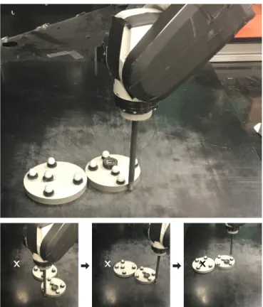
Fig. 1: Top: the robot wants to push the second disk to a goal position by pushing on the first disk. Bottom: three snapshots within a successful push (target marked as X). The robot learns to first push the first disk to the right and then use it to push the second disk to the target position.
easier and more sample efficient than learning from scratch. This approach has been shown to be more data efficient, have better generalization capabilities, and outperform its purely analytical or data-driven counterparts [8], [9], [10], [11].
Most residual-based approaches assume a fixed number of objects in the world states. This means they cannot be applied to states with a varied number of objects or generalize what they learn for one object to other similar ones. This problem has been addressed by approaches that use graph-structured network models, such as interaction networks [12] and neural physics engines [13]. These methods are effective at generalizing over objects, modeling interactions, and handling variable numbers of objects. However, as they are purely data-driven, in practice they require a large number of training examples to arrive at a good model.
In this paper, we propose simulator-augmented interaction networks (SAIN), incorporating interaction networks into a physical simulator for complex, real-world control problems. Specifically, we show:
• Sample-efficient residual learning and improved predic-tion accuracy relative to the physics engine,
• Accurate predictions for the dynamics and interaction of novel arrangements and numbers of objects, and the
• Utility of the learned residual model for control in highly underactuated planar pushing tasks.
We demonstrate SAIN’s performance on the experimental setup depicted in Fig. 1. Here, the robot’s objective is to guide the second disk to a goal by pushing on the first. This task is challenging due to the presence of multiple complex frictional interactions and underactuation [14]. We demonstrate the step-by-step deployment of SAIN, from training in simulation to augmentation with real-world data, and finally control.
II. RELATEDWORK
A. Learning Contact Dynamics
In the field of contact dynamics, researchers have looked towards data-driven techniques to complement analytical models and/or directly learn dynamics. For example, Byravan and Fox [15] designed neural nets to predict rigid-body motions for planar pushing. Their approach does not exploit explicit physical knowledge. Kloss et al. [11] used neural net predictions as input to an analytical model; the output of the analytical model is used as the prediction. Here, the neural network learns to maximize the analytical model’s perfor-mance. Fazeli et al. [8] also studied learning a residual model for predicting planar impacts. Zhou et al. [16] employed a data-efficient algorithm to capture the frictional interaction between an object and a support surface. They later extended it for simulating parametric variability in planar pushing and grasping [17].
The paper closest to ours is that from Ajay et al. [9], where they used the analytical model as an approximation to the push outcomes, and learned a residual neural model that makes corrections to its output. In contrast, our paper makes two key innovations: first, instead of using a feedforward network to model the dynamics of a single object, we employ an object-based network to learn residuals. Object-object-based networks build upon explicit object representations and learn how they interact; this enables capturing multi-object interactions. Second, we demonstrate that such a hybrid dynamics model can be used for control tasks both in simulation and on a real robot.
B. Differentiable Physical Simulators
There has been an increasing interest in building differ-entiable physics simulators [18]. For example, Degrave et al. [19] proposed to directly solve differentiable equations. Such systems have been deployed for manipulation and planning for tool use [20]. Battaglia et al. [12] and Chang et al. [13] have both studied learning object-based, differentiable neural simulators. Their systems explicitly model the state of each object and learn to predict future states based on object interactions. In this paper, we combine such a learned object-based simulator with a physics engine for better prediction and for controlling real-world objects.
C. Control with a Learned Simulator
Recent papers have explored model-predictive control with deep networks [21], [22], [23], [24], [25]. These approaches learn an abstract-state transition function, not an explicit model of the environment [26], [27]. Eventually, they apply the learned value function or model to guide policy network training. In contrast, we employ an object-based physical simulator that takes raw object states (e.g., velocity, position) as input. Hogan et al. [28] also learned a residual model with an analytical model for model-predictive control, but their learned model is a task-specific Gaussian Process, while our model has the ability to generalize to new object shapes and materials.
A few papers have exploited the power of interaction networks for planning and control, mostly using interaction networks to help training policy networks via imagination— rolling out approximate predictions [29], [30], [31]. In contrast, we use interaction networks as a learned dynamics simulator, combine it with a physics engine, and directly search for actions in real-world control problems. Recently, Sanchez-Gonzalez et al. [32] also used interaction networks in control, though their model does not take into account explicit physical knowledge, and its performance is only demonstrated in simulation.
III. METHOD
In this section, we describe SAIN’s formulation and components. We also present our Model Predictive Controller (MPC) which uses SAIN to perform the pushing task.
A. Formulation
Let S be the state space and A be the action space. A dynamics model is a function f : S × A → S that predicts the next state given the current action and state: f (s, a) ≈ s0, for all s, s0 ∈ S, a ∈ A.
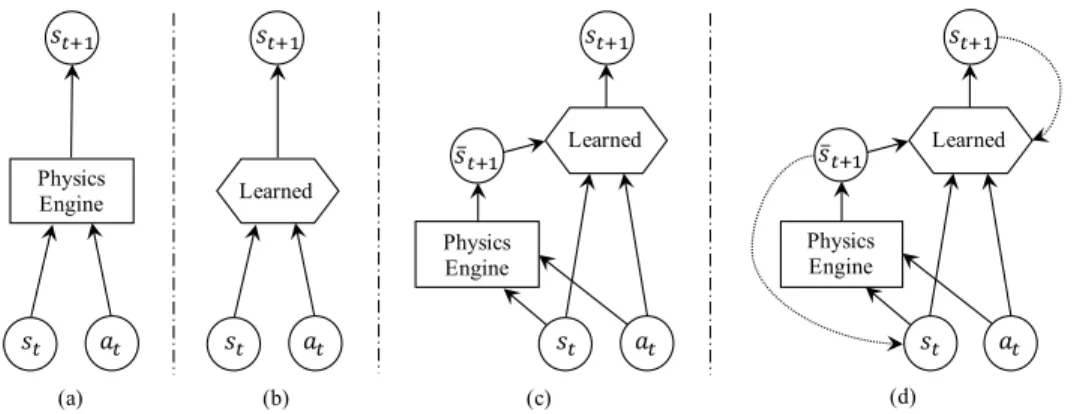
There are two general types of dynamics models: analytical (Fig. 2a) and data-driven (Fig. 2b). Our goal is to learn a hybrid dynamics model that combines the two (Fig. 2c). Here, conditioned on the state-action pair, the data-driven model learns the discrepancy between analytical model predictions and real-world data (i.e. the residual). Specifically, let fr
represent the hybrid dynamics model, fprepresent the physics
engine, and fθ represent the residual component. We have
fr(s, a) = fθ(fp(s, a), s, a) ≈ s0. Intuitively, the residual
model refines the physics engine’s guess using the current state and action.
For long-term prediction, let fθR: S ×S ×A → S represent the recurrent hybrid dynamics model (Fig. 2d). If s0 is the
initial state, at the action at time t, ¯stthe prediction by the
physics engine fp at time t and ˆstthe prediction at time t,
then
fθR(¯st+1, ˆst, at) = ˆst+1≈ st+1, (1)
𝑠" 𝑠"#$ Physics Engine 𝑠"#$ Learned Physics Engine 𝑠"#$ Learned (a) (b) (c) 𝑠̅"#$ 𝑎" 𝑠" 𝑎" 𝑠" 𝑎" Physics Engine 𝑠"#$ Learned (d) 𝑠̅"#$ 𝑠" 𝑎"
Fig. 2: Model classes: (a) physics-based analytical models; (b) data-driven models; (c) simulator-augmented residual models; (d) recurrent simulator-augmented residual models.
For training, we collect observational data {(st, at, st+1)}T −1t=0
and then solve the following optimization problem:
θ∗= arg min θ T −1 X t=0 kˆst+1− st+1k22+λkθk 2 2, (3)
where λ is the weight for the regularization term.
In this study, we choose to use a recurrent parametric model over a non-recurrent representation for two reasons. First, non-recurrent models are trained on observation data to make single-step predictions. Consequently, errors in prediction compound over a sequence of steps. Second, since these models recursively use their own predictions, the input data given during the simulation phase will have a different distribution than the input data during the training phase. This creates a data distribution mismatch between the training and test phases.
B. Interaction Networks
We use interaction networks [12] as the data-driven model for multi-object interaction. An interaction network consists of 2 neural nets: fdyn and frel. The frel network
calculates pairwise forces between objects and the fdyn
network calculates the next state of an object, based on the states of the objects it is interacting with and the nature of the interactions.
The original version of interaction networks was trained to make a single-step prediction; for improved accuracy, we extend them to make multi-step predictions. Let st =
{o1 t, o
2 t, . . . , o
n
t} be the state at time t, where o i
t is the state
for object i at time t. Similarly, let ˆst= {ˆo1t, ˆo2t, . . . , ˆont} be
the predicted state at time t where oitis the predicted state
for object i at time t. In our work, oit= [pit, vit, mi, ri] where
pi
tis the pose of object i at time step t, vit the velocity of
object i at time step t, mi the mass of object i and ri the radius of object i. Similarly, ˆoi
t = [ˆpit, ˆvti, mi, ri] where ˆpit
is the predicted pose of object i at time step t and ˆvi t the
predicted velocity of object i at time step t. Note that we do not predict any changes to static object properties such as mass and radius. Also, we note that while st is a set of
objects, the state of any individual object, oi
t, is a vector.
Now, let ai
t be the action applied to object i at time t. The
equations for the interaction network are: eit=X j6=i frel(vit, p i t− p j t, v i t− v j t, m i, mj, ri, rj), (4) ˆ vt+1i = vit+ dt · fdyn(vti, a i t, m i, ri, ei t), (5) ˆ pit+1= pit+ dt · ˆvit+1, (6) ˆ oit+1= [ˆpit+1, ˆvt+1i , mi, ri]. (7) C. Simulator-Augmented Interaction Networks (SAIN)
A simulator-augmented interaction network extends an interaction network, where fdyn and frel now take in the
prediction of a physics engine, fp. We now learn the residual
between the physics engine and the real world. Let ¯st =
{¯o1
t, ¯o2t, . . . , ¯ont} be the state at time t and ¯oit be the state
for object i at time t predicted by the physics engine. The equations for SAIN are
¯ st+1= fp(¯st, a1t, a 2 t, . . . , a n t), (8) eit=X j6=i frel(vit, ¯v i t+1− ¯v i t, p i t− p j t, v i t− v j t, m i, mj, ri, rj), (9) ˆ vt+1i = vit+ dt × fdyn(vit, ¯p i t+1− ¯p i t, a i t, m i, ri, ei t), (10) ˆ pit+1= pit+ dt × ˆvt+1i , (11) ˆ oit+1= [ˆpit+1, ˆvit+1, mi, ri]. (12) These equations describe a single-step prediction. For multi-step prediction, we use the same equations by providing the true state s0 at t = 0 and predicted state ˆst at t > 0 as input.
D. Control Algorithm
Our action space has two free parameters: the point where the robot contacts the first disk and the direction of the push. In our experiments, a successful execution requires searching for a trajectory of about 50 actions. Due to the size of the search space, we use an approximate receding horizon control algorithm with our dynamics model. The search algorithm maintains a priority queue of action sequences based on the heuristic below. For each expansion, let st be the current
state and ˆst+T(at, . . . , at+T −1) be the predicted state after
T steps with actions at, . . . , at+T −1. Let sg be the goal state.
We choose the control strategy at that minimizes the the
the new action sequence into the queue. IV. EXPERIMENTS
We demonstrate SAIN on a challenging planar manipula-tion task both in simulamanipula-tion and in the real-world. We further evaluate how our model generalizes to handle control tasks that involve objects of new materials and shapes.
A. Task
In this manipulation task, we are given two disks with different mass and radii. Our goal is to guide the second disk to a target location, but are constrained to push only the first disk. Here, a point s in the state space is factored into a set of two object states, s = {o1, o2}, where each oi is an
element of object state space O. The object state includes the mass, 2D position, rotation, velocity, and radius of the disk.
Targets locations are generated at random and divide into two categories: easy and hard. A target location is produced by first sampling an angle α from an interval U , then choosing the goal location to be at distance of three times the radius of second disk and at an angle of α with respect to the second disk. In easy pushes, the interval U is [−π6,π
6]. In
hard pushes, the interval U is [−π3, −π6] ∪ [π6,π3]. A push is considered a success if the distance between the goal location and the pose of the center of mass of the second disk is within 101th the radius of second disk.
B. Simulation Setup
We use the Bullet physics engine [33] for simulation. For each trajectory, we vary the coefficient of friction between the surface and the disks, the mass of the disks and their radius. The coefficient of friction is sampled from Uniform(0.05, 0.25). The mass is sampled from Uni-form(0.85kg, 1.15kg) and the radius is sampled from Uniform(0.05m, 0.06m). We always fix the initial position of the first disk to the origin. The other disks are placed in front of the first disk at an angle, randomly sampled from Uniform(−π3,π3), and just touches it. We ensure that disks don’t overlap each other. The pusher is placed at back of the first disk at an angle randomly sampled from Uniform(−π3,π3), and just touches it. Then the pusher makes a straight line push at an angle, randomly sampled from Uniform(−π6,π6), for 2s and covers a distance of about 1cm. We experiment with two different simulation setups: (1) direct-force simulation setup in which we control pusher with external force and (2) robot control simulation setup in which we control the pusher using position control. We use the first setup to show the benefits of SAIN over other models. But in our real world setup, we control the pusher using position-based control. So, we have designed a second simulation setup which matches the real robot and use it to collect pre-training data.
For the direct-force simulation setup, we collect 4500 pushes with 2 disks for our training set, 500 pushes with 2 disks and 500 pushes with 3 disks for our test set. For the robot control simulation setup, we collect 4500 pushes with
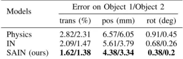
Models Error on Object 1/Object 2 trans (%) pos (mm) rot (deg) Physics 2.82/2.31 6.57/6.05 0.91/0.45 IN 2.09/1.47 5.61/3.79 0.68/0.26 SAIN (ours) 1.62/1.38 4.38/3.34 0.38/0.2
TABLE I: Errors on dynamics prediction in direct-force simu-lation setup. SAIN achieves the best performance in both position and rotation estimation, compared with methods that rely on physics engines or neural nets alone. The first two metrics are the average Euclidean distance between the predicted and the ground truth object reported as a percentage relative to the initial pose (trans) and as absolute values (pos) in millimeters. The third is the average error of object rotation (rot) in degree.
2 disks for our training set and 500 pushes with 2 disks for our test set.
C. Model and Implementation Details
We compare two models for simulation and control: the original interaction networks (IN) and our simulator-augmented interaction networks (SAIN). They share the same architecture. Each consists of two separate neural networks: fdyn and frel. Both fdyn and frel have four linear layers with
hidden sizes of 128, 64, 32 and 16 respectively. The first three linear layers are followed by a ReLU activation.
Training interaction networks in simulation is straightfor-ward. It is more involved for SAIN, which learns a correction over the Bullet physics engine, so the problem of training “in simulation” is ill-posed. To address this problem, we fix the physics engine in SAIN with mass and radius of disks equaling that of disks in the real world. We also fix the coefficient of friction in the physics engine to an estimated mean of the coefficient of friction of the real world surface across space. The training data instead contain varied mass and radius of both disks, and varied the coefficient of friction between the disks and the surface, and the model is trained to learn the residual.
We use ADAM [34] for optimization with a starting learning rate of 0.001. We decrease it by 0.5 every 2,500 iterations. We train these models for 10,000 iterations with a batch size of 100. Let the predicted 2D position, rotation, and velocity at time t of disk i be ˆpi
t, ˆrti and ˆvit, respectively,
and the corresponding true values be pit, rti, and vit. Let T
be the length of all trajectories. The training loss function for a single trajectory is
(13) 1 T 2 X i =1 T −1 X t =0 kpit− ˆp i tk 2 2+ kv i t− ˆv i tk 2 2+ ksin (ri t) − sin (ˆr i t)k 2 2+ kcos (r i t) − cos (ˆr i t)k 2 2.
During training, we use a batch of trajectories and take a mean over the loss of those trajectories. We also use l2
regularization with 10−3 as regularization constant.
In practice, we ask the models to predict the change in object states (relative values) rather than the absolute values. This enables them to generalize to arbitrary starting positions without overfitting.
Models Error on Object 1/2/3
trans (%) pos (mm) rot (deg) Physics 2.79/2.34/2.38 6.53/6.11/6.21 0.89/0.48/0.49 IN 2.12/1.63/1.67 5.68/4.41/4.52 0.70/0.34/0.38 SAIN (ours) 1.68/1.52/1.61 4.54/3.97/4.34 0.41/0.25/0.32 TABLE II: Generalization to 3 objects in direct-force simulation setup. SAIN achieves the best generalization in both position and rotation estimation.
Models Error on Object 1/2 trans (%) pos (mm) rot (deg) Physics 2.52/2.19 6.27/5.81 0.85/0.29 IN 2.13/1.59 5.76/3.84 0.72/0.28 SAIN (ours) 1.82/1.50 4.66/3.47 0.40/0.21 TABLE III: Errors on dynamics prediction in robot control simulation setup. SAIN achieves the best performance in both position and rotation estimation.
D. Search Algorithm
As mentioned in Sec. III-D, an action is defined by the initial position of the pusher and the angle of the push, α, with respect to the first disk. After these parameters have been selected, the pusher starts at the initial position and moves at an angle of α with respect to the first disk for 10mm. We discretize our action space as follows. For selecting α, we divide the interval [−π6 ,π
6] into six bins and choose their
midpoints. For selecting the initial position of the pusher, we choose an angle θ and place the pusher at edge of first disk at an angle θ such that the pusher touches the first disk. For selecting θ, we divide the interval [−π3 ,π3] into 12 bins and choose midpoint of one of these bins. Therefore, our action space consists of 72 discretized actions for each time step. We maintain a priority queue of action sequences based on heuristic h(ˆp1, ˆp2, pg) where ˆpi is the predicted 2D position
of disk i and pg is the 2D position of goal. h(ˆp1, ˆp2, pg) is
sum of kˆp2− pgk and cosine distance between pg− ˆp1 and
ˆ
p2− ˆp1. The cosine distance serves as a regularization cost to encourage the center of both disks and the goal to stay in a straight line. To prevent the priority queue from blowing up, we do receding horizon greedy search with an initial horizon of 2, and increase it to 3 when the distance between the second disk and goal is less than 10mm.
E. Prediction and Control Results in Simulation
The forward multi-step prediction errors of both interaction networks and SAIN for direct-force simulation setup with 2 disks and 3 disks are reported in Table I and Table II. Note that errors on different objects are separated by / in all the tables. The training data for this setup consist of pushes with only 2 disks. The forward multi-step prediction errors of both interaction networks and SAIN for robot control simulation setup are reported in Table III. Given an initial state and a sequence of actions, the models do forward prediction for the next 200 timesteps, where each time-step is 1/240s. We see that SAIN outperforms interaction networks in both setups. We also list the results of the fixed physics engine used for training SAIN for reference.
Models Fine-tuning Error on Object 1/2 trans (%) pos (mm) rot (deg) Physics N/A 0.87/1.91 3.06/6.41 0.32/0.17 IN No 0.86/1.84 2.96/5.75 0.96/0.32 SAIN (ours) No 0.69/1.06 2.38/3.52 0.43/0.18 IN Yes 0.63/0.61 2.23/2.05 0.41/0.19 SAIN (ours) Yes 0.42/0.43 1.50/1.52 0.34/0.17 TABLE IV: Errors on dynamics prediction in the real world. SAIN obtains the best performance in both position and rotation estimation. Its performance gets further improved after fine-tuning on real data.
(a) Control with interaction networks (IN)
(b) Control with simulator-augmented interaction networks (SAIN) Models Easy Push Hard Push
IN 100% 88%
SAIN (ours) 100% 100%
Fig. 3: Qualitative results and success rates on control tasks in simulation. The goal is to push the red disk so that the center of the blue disk reaches the target region (yellow). The transparent shapes are their initial positions, and the solid ones are their final positions after execution. The center of the blue disk after execution is marked as a white cross. (a) Control with interaction networks works well but makes mistakes occasionally (column 3). (b) Control with SAIN achieves perfect performance in simulation.
We have also evaluated IN and SAIN on control tasks in simulation. We test each model on 25 easy and 25 hard pushes. For these pushes, we set the mass of two disks to 0.9kg and 1kg and their radius to 54mm and 59mm, making them differ them from those used in the internal physics engine of SAIN. This mimics real-world environments, where objects’ size and shape cannot be precisely estimated, and ensures SAIN cannot cheat by just querying the internal simulator. Fig. 3 shows SAIN performs better than IN. This suggests learning the residual not only helps to do better forward prediction, but also benefits control.
F. Real-World Robot Setup
We now test our models on a real robot. The setup used for the real experiments is based on the system from the MIT Push dataset [4]. The pusher is a cylinder of radius 4.8mm attached to the last joint of a ABB IRB 120 robot. The position of the pusher is recorded using the robot kinematics. The two disks being pushed are made of stainless steel, have radius of
(a) Using the model trained on simulated data only
(b) Using the model trained on both simulated and real data Model Data Easy Push Hard Push
SAIN Sim 100% 68%
SAIN Sim + Real 100% 96%
Fig. 4: Qualitative results and success rates on control tasks in the real world. The goal is to push the red disk so that the center of the blue disk reaches the target region (yellow). The left column is an example of easy pushe, while the right two show hard pushes. (a) The model trained on simulated data only performs well for easy pushes, but sometimes fails on harder control tasks; (b) The model trained on simulated and real data improves the performance, working well for both easy and hard pushes.
(a) Results on a new surface
(b) Results on a new shape with a smaller radius Fig. 5: Generalization to new scenarios. (a) SAIN trained gener-alizes to control tasks on a new surface (plywood), with a success rate of 92%; (b): It also generalizes to tasks where the two disks have a different radius (red: small → large; blue: large → small), with a success rate of 88%. All tasks here are hard pushes.
52.5mm and 58mm, and weight 0.896kg and 1.1kg. During the experiments, the smallest disk is the one pushed directly by the pusher. The position of both disks is tracked using a Vicon system of four cameras so that the disks’ positions are highly accurate. Finally, the surface where the objects lay is made of ABS (Acrylonitrile Butadiene Styrene), whose coefficient of friction is around 0.15. Each push is done at 50mm/s and spans 10mm. We collect 1,500 pushes out of which 1,200 are used for training and 300 for testing.
We evaluate two versions of interaction networks and SAIN. The first is an off-the-shelf version purely trained on synthetic
data; the second is one trained on simulated data and later fine-tuned on real data. This helps us understand whether these models can exploit real data to adapt to new environments. G. Results on Real-World Data
Results of forward simulation are shown in Table IV. SAIN outperforms IN on real data. While both models benefit from fine-tuning, SAIN achieves the best performance. This suggests residual learning also generalizes to real data well. All models achieve a lower error on real data than in simulation; this is because simulated data have a significant amount of noise to make the problem more challenging.
We then evaluate SAIN (both with and without fine-tuning) for control, on 25 easy and 25 hard pushes. The results are shown in Fig. 4. The model without fine-tuning achieves 100% success rate on easy pushes and 68% on hard pushes. As shown in the rightmost columns of Fig. 4a, it sometimes pushes the object too far and gets stuck in a local minimum. After fine-tuning, the model works well on both easy pushes (100%) and hard pushes (96%) (Fig. 4b).
While objects of different shapes and materials have differ-ent dynamics, the gap between their dynamics in simulation and in the real world might share similar patterns. This is the intuition behind the observation that residual learning allows easier generalization to novel scenarios. Ajay [9] validated this for forward prediction. Here, we evaluate how our fine-tuned SAIN generalizes for control. We test our model on 25 hard pushes with a different surface (plywood, where the original surface is ABS), using the original disks. Our framework achieves successes in 92% of the pushes, where Fig. 5a shows qualitative results. We’ve also evaluated our model on another 25 hard pushes, where it pushes the large disk (58mm) to direct the small one (52.5mm). Our framework achieves successes in 88% of the pushes. Fig. 5b shows qualitative results. These results suggest that SAIN can generalize to solve control tasks with new object shapes and materials.
V. CONCLUSION
We have proposed a hybrid dynamics model, simulator-augmented interaction networks (SAIN), combining a physical simulator with a learned, object-centered neural network. Our underlying philosophy is to first use analytical models to model real-world processes as much as possible, and learn the remaining residuals. Learned residual models are specific to the real-world scenario for which data is collected, and adapt the model accordingly. The combined physics engine and residual model requires little need for domain specific knowledge or hand-crafting and can generalize well to unseen situations. We have demonstrated SAIN’s efficacy when applied to a challenging control problem in both simulation and the real world. Our model also generalizes to setups where object shape and material vary and has potential applications in control tasks that involve complex contact dynamics. Acknoledgements. This work is supported by NSF #1420316, #1523767, and #1723381, AFOSR grant FA9550-17-1-0165, ONR MURI N00014-16-1-2007, Honda Research, Facebook, and Draper Laboratory.
REFERENCES
[1] E. Todorov, T. Erez, and Y. Tassa, “Mujoco: A physics engine for
model-based control,” in IROS. IEEE, 2012, pp. 5026–5033.
[2] E. Coumans, “Bullet physics simulation,” in SIGGRAPH, 2015. [3] R. Kolbert, N. Chavan Dafle, and A. Rodriguez, “Experimental
Validation of Contact Dynamics for In-Hand Manipulation,” in ISER, 2016.
[4] K.-T. Yu, M. Bauza, N. Fazeli, and A. Rodriguez, “More than a million ways to be pushed. a high-fidelity experimental dataset of
planar pushing,” in IROS. IEEE, 2016, pp. 30–37.
[5] N. Fazeli, S. Zapolsky, E. Drumwright, and A. Rodriguez, “Fundamen-tal limitations in performance and interpretability of common planar rigid-body contact models,” in ISRR, 2017.
[6] I. Mordatch, K. Lowrey, and E. Todorov, “Ensemble-cio: Full-body dynamic motion planning that transfers to physical humanoids,” in IROS, 2015.
[7] A. Becker and T. Bretl, “Approximate steering of a unicycle under bounded model perturbation using ensemble control,” IEEE TRO, vol. 28, no. 3, pp. 580–591, 2012.
[8] N. Fazeli, S. Zapolsky, E. Drumwright, and A. Rodriguez, “Learning data-efficient rigid-body contact models: Case study of planar impact,” in CoRL, 2017, pp. 388–397.
[9] A. Ajay, J. Wu, N. Fazeli, M. Bauza, L. P. Kaelbling, J. B. Tenenbaum, and A. Rodriguez, “Augmenting physical simulators with stochastic neural networks: Case study of planar pushing and bouncing,” in IROS, 2018.
[10] K. Chatzilygeroudis and J.-B. Mouret, “Using parameterized black-box priors to scale up model-based policy search for robotics,” in ICRA, 2018.
[11] A. Kloss, S. Schaal, and J. Bohg, “Combining learned and analytical models for predicting action effects,” arXiv:1710.04102, 2017. [12] P. W. Battaglia, R. Pascanu, M. Lai, D. Rezende, and K. Kavukcuoglu,
“Interaction networks for learning about objects, relations and physics,” in NeurIPS, 2016.
[13] M. B. Chang, T. Ullman, A. Torralba, and J. B. Tenenbaum, “A compositional object-based approach to learning physical dynamics,” in ICLR, 2017.
[14] F. R. Hogan and A. Rodriguez, “Feedback control of the pusher-slider system: A story of hybrid and underactuated contact dynamics,” in WAFR, 2016.
[15] A. Byravan and D. Fox, “Se3-nets: Learning rigid body motion using deep neural networks,” in ICRA, 2017.
[16] J. Zhou, R. Paolini, A. Bagnell, and M. T. Mason, “A convex polynomial force-motion model for planar sliding: Identification and application,” in ICRA, 2016, pp. 372–377.
[17] J. Zhou, A. Bagnell, and M. T. Mason, “A fast stochastic contact model for planar pushing and grasping: Theory and experimental validation,” in RSS, 2017.
[18] S. Ehrhardt, A. Monszpart, N. Mitra, and A. Vedaldi, “Taking visual motion prediction to new heightfields,” arXiv:1712.09448, 2017. [19] J. Degrave, M. Hermans, and J. Dambre, “A differentiable physics
engine for deep learning in robotics,” in ICLR Workshop, 2016. [20] M. Toussaint, K. Allen, K. Smith, and J. Tenenbaum, “Differentiable
physics and stable modes for tool-use and manipulation planning,” in RSS, 2018.
[21] I. Lenz, R. A. Knepper, and A. Saxena, “Deepmpc: Learning deep latent features for model predictive control,” in RSS, 2015.
[22] S. Gu, T. Lillicrap, I. Sutskever, and S. Levine, “Continuous deep q-learning with model-based acceleration,” in ICML, 2016. [23] A. Nagabandi, G. Kahn, R. S. Fearing, and S. Levine, “Neural network
dynamics for model-based deep reinforcement learning with model-free fine-tuning,” in ICRA, 2018.
[24] G. Farquhar, T. Rockt¨aschel, M. Igl, and S. Whiteson, “Treeqn and atreec: Differentiable tree planning for deep reinforcement learning,” in ICLR, 2018.
[25] A. Srinivas, A. Jabri, P. Abbeel, S. Levine, and C. Finn, “Universal planning networks,” in ICML, 2018.
[26] D. Silver, H. van Hasselt, M. Hessel, T. Schaul, A. Guez, T. Harley, G. Dulac-Arnold, D. Reichert, N. Rabinowitz, A. Barreto, and T. Degris, “The predictron: End-to-end learning and planning,” in ICML, 2017. [27] J. Oh, S. Singh, and H. Lee, “Value prediction network,” in NeurIPS,
2017.
[28] M. Bauza, F. R. Hogan, and A. Rodriguez, “A data-efficient approach to precise and controlled pushing,” in CoRL, 2018.
[29] S. Racani`ere, T. Weber, D. Reichert, L. Buesing, A. Guez, D. J. Rezende, A. P. Badia, O. Vinyals, N. Heess, Y. Li, R. Pascanu, P. Battaglia, D. Silver, and D. Wierstra, “Imagination-augmented agents for deep reinforcement learning,” in NeurIPS, 2017.
[30] J. B. Hamrick, A. J. Ballard, R. Pascanu, O. Vinyals, N. Heess, and P. W. Battaglia, “Metacontrol for adaptive imagination-based optimization,” in ICLR, 2017.
[31] R. Pascanu, Y. Li, O. Vinyals, N. Heess, L. Buesing, S. Racani`ere, D. Reichert, T. Weber, D. Wierstra, and P. Battaglia, “Learning model-based planning from scratch,” arXiv:1707.06170, 2017.
[32] A. Sanchez-Gonzalez, N. Heess, J. T. Springenberg, J. Merel, M. Ried-miller, R. Hadsell, and P. Battaglia, “Graph networks as learnable physics engines for inference and control,” in ICML, 2018.
[33] E. Coumans, “Bullet physics engine,” Open Source Software: http://bulletphysics. org, 2010.
[34] D. P. Kingma and J. Ba, “Adam: A method for stochastic optimization,” in ICLR, 2015.