New Simulation Techniques in Kinship Network Analysis

HAL Id: halshs-01429067

https://halshs.archives-ouvertes.fr/halshs-01429067

HAL is a multi-disciplinary open access archive for the deposit and dissemination of sci-entific research documents, whether they are pub-lished or not. The documents may come from teaching and research institutions in France or abroad, or from public or private research centers.

L’archive ouverte pluridisciplinaire HAL, est destinée au dépôt et à la diffusion de documents scientifiques de niveau recherche, publiés ou non, émanant des établissements d’enseignement et de recherche français ou étrangers, des laboratoires publics ou privés.

To cite this version:

Telmo Menezes, Floriana Gargiulo, Camille Roth, Klaus Hamberger. New Simulation Techniques in Kinship Network Analysis. Structure and Dynamics : e-Journal of Anthropological and Related Sciences, University of California, 2016, 9 (2), pp.180-209. �halshs-01429067�

eScholarship provides open access, scholarly publishing services to the University of California and delivers a dynamic research platform to scholars worldwide.

Peer Reviewed Title:

New Simulation Techniques in Kinship Network Analysis Journal Issue:

Structure and Dynamics, 9(2) Author:

Menezes, Telmo, An-Institut der Humboldt Universität Gargiulo, Floriana, University of Namur

Roth, Camille, An-Institut der Humboldt Universität

Hamberger, Klaus, Ecole des Hautes Etudes en Sciences Sociales Publication Date:

2016 Permalink:

http://escholarship.org/uc/item/5p57j1jm Acknowledgements:

This work has been partially supported by the French National Agency of Research (ANR) through grant “SIMPA” ANR-09-SYSC-013-02. The paper has benefited from regular interactions with the members of the research group TIP (Traitement Informatique de la Parenté—Kinship and Computing, www.kintip.net). We are particularly grateful to Isabelle Daillant, who has not only generously allowed us to use her Chimane dataset, but also much helped to improve the paper by her careful critical reading. We also thank the reviewers of Structure and Dynamics for their numerous helpful comments and suggestions. All errors, of course, are ours.

Author Bio:

Centre Marc Bloch Berlin NaXys

Centre Marc Bloch Berlin e.V. Laboratoire d’Anthropologie Sociale Keywords:

Kinship, Computer Simulation, Marriage Networks Local Identifier:

eScholarship provides open access, scholarly publishing services to the University of California and delivers a dynamic research platform to scholars worldwide.

features, it is now easy to produce a complete census of matrimonial circuits, both between individuals and between groups. However, the abundance of structural features which have thus become accessible raises a new question: to what extent can they be taken as indicators of sociological phenomena (such as marriage preferences or avoidances), rather than as effects of chance or of observer bias?

This paper presents a series of recently developed simulation techniques that deal with this issue. Starting from a new approach to “classical” agent-based modeling of kinship and alliance (group) networks (Section 2), we then present an automatic model discovery technique which, instead of constructing alliance networks from given matrimonial rules, reconstructs plausible matrimonial rules underlying given alliance networks (Section 3). While these techniques apply to “objective” representations of kinship and alliance networks, we also present two methods that take into account the generally lacunar and biased character of empirical kinship datasets. The first method we propose to deal with this problem (Section 4) is a generalized version of White’s (1999) “reshuffling” approach, which consists in redistributing marriage or descent links between individuals or groups while keeping the numbers of links constant. (For alliance networks, the question can be dealt with analytically by straightforward calculation of expected marriage circuit frequencies.) The second method (Section 5) consists in simulating the processes of network exploration by a virtual fieldworker navigating through kinship or alliance networks according to given behavioral constraints.

Copyright Information:

Copyright 2016 by the article author(s). This work is made available under the terms of the Creative Commons Attribution3.0 license, http://creativecommons.org/licenses/by/3.0/

NEW SIMULATION TECHNIQUES IN KINSHIP

NETWORK ANALYSIS

Telmo Menezes

Centre Marc Bloch Berlin

(An-Institut der Humboldt Universität)

Friedrichstr. 191, 10117 Berlin, Germany

menezes@cmb.hu-berlin.de

Floriana Gargiulo

NaXys, University of Namur

8 rempart de la vierge, B5000, Namur, Belgium

floriana.gargiulo@gmail.com

Camille Roth

Centre National de Recherche Scientifique

Centre Marc Bloch Berlin e.V.

(An-Institut der Humboldt Universität)


Friedrichstr. 191, 10117 Berlin, Germany


roth@cmb.hu-berlin.de

Klaus Hamberger

Ecole des Hautes Etudes en Sciences Sociales

Laboratoire d’Anthropologie Sociale

3 Rue d’Ulm, 75005 Paris, France

klaus.hamberger@ehess.fr

0. Introduction

In the enterprise of confronting kinship theories (and indigenous kinship norms) with matrimonial practice, simulation techniques have, from the very beginning, played a cen-tral role. When computer tools were first introduced into social anthropology in the 1960s, simulation was one of the main techniques (Fischer 2004: 184, cf. Dyke 1981, Wright 2000, Fischer and Kronenfeld 2011), and marriage systems were among its first applications. The first anthropological article using simulation (Kunstadter et al. 1963) dealt with the feasibility of prescribed matrilateral cross-cousin marriage, and Gilbert and Hammel (1966) used it to demonstrate that agnatic first cousin marriages could be an epiphenomenon of territorial endogamy rather than an expression of direct matrimonial preferences.

Despite the initial focus on matrimonial norms and practices, these soon ceased to be an object of interest in their own right. When simulation techniques implemented as-sumptions about marriage rules, incest prohibitions, monogamy, and so on, the goal was generally to study their impact on other variables, such as population growth (MacCluer and Dyke 1976, Black 1978), the extension of personal kindreds (Wachter et al. 1997,

Thanks to new conceptual and computational tools, the analysis of kinship and mar-riage networks has advanced considerably over the past twenty-five years. While in the past, the discussion of empirical marriage practices was often restricted to a casual observation of salient network features, it is now easy to produce a complete census of matrimonial circuits, both between individuals and between groups. However, the abun-dance of structural features which have thus become accessible raises a new question: to what extent can they be taken as indicators of sociological phenomena (such as mar-riage preferences or avoidances), rather than as effects of chance or of observer bias? This paper presents a series of recently developed simulation techniques that deal with this issue. Starting from a new approach to “classical” agent-based modeling of kinship and alliance (group) networks (Section 2), we then present an automatic model discov-ery technique which, instead of constructing alliance networks from given matrimonial rules, reconstructs plausible matrimonial rules underlying given alliance networks (Sec-tion 3). While these techniques apply to “objective” representa(Sec-tions of kinship and al-liance networks, we also present two methods that take into account the generally lacu-nar and biased character of empirical kinship datasets. The first method we propose to deal with this problem (Section 4) is a generalized version of White’s (1999) “reshuf-fling” approach, which consists in redistributing marriage or descent links between in-dividuals or groups while keeping the numbers of links constant. (For alliance net-works, the question can be dealt with analytically by straightforward calculation of ex-pected marriage circuit frequencies.) The second method (Section 5) consists in simulat-ing the processes of network exploration by a virtual fieldworker navigatsimulat-ing through kinship or alliance networks according to given behavioral constraints.

Murphy 2010), the spatial diffusion of genes (Murphy et al. 1994) or the interaction of social and ecological systems (Christiansen and Altaweel 2005, McAllister et al. 2005). In contrast, studies using agent-based simulation to analyze the internal logic of kinship systems and to test simulation predictions against ethnographic data (Fischer 1986, 2006, Read 1998, Small 2000, White et al. 2006, Geller et al. 2011) are still relatively rare.

One reason for the scarcity of agent-based simulations based on realistic models of kinship networks is the highly complex nature of the genealogical datasets used by so-cial scientists. Not only do numerous demographic and sociological factors (fertility and mortality rates, marriage and residence preferences, spatial distribution and migration, etc.) jointly affect the form of real-world kinship networks, the datasets collected by so-cial scientists are generally subject to (often substantial) observer bias and thus cannot be taken as miniature images faithfully reproducing the morphology of the actual networks from which they are obtained.

In this survey article, we discuss several recently developed simulation techniques designed to deal with the problem posed by the multiplicity of (agent- and observer-relat-ed) factors affecting the generation of kinship and marriage links. All result from the re-search project “Simulations de la Parenté—Kinship Simulations.” 1

After presenting a new technique for doing “classical” agent-based modeling of kinship and alliance (group) networks (Section 2), we will then introduce an automatic model discovery technique that, instead of constructing alliance networks from matrimo-nial rules, reconstructs matrimomatrimo-nial rules underlying the empirical alliance networks (Section 3). While these techniques (both in their “direct” and in their “reverse” form) apply to “objective” representations of kinship and alliance networks, we then introduce methods for taking into account the generally lacunar and biased character of empirical kinship datasets. The first method (Section 4) is a generalized version of White’s (1999) “reshuffling” approach and consists in redistributing marriage or descent links between individuals or groups, while keeping the number of links constant. (For alliance net-works, the question can be dealt with analytically by straightforward calculation of ex-pected marriage circuit frequencies.) The second method (Section 5) consists in simulat-ing the processes of network exploration by a virtual fieldworker navigatsimulat-ing through kin-ship or alliance networks according to given behavioral constraints.

All the techniques presented in this article have been implemented in the open sourcesoftware Puck. 2

1. The Framework 1.1. Basic Concepts

We first specify several basic concepts that we will use throughout this article. First is a 3

distinction between kinship (or genealogical) networks and alliance networks. Both kinds of networks are graphs that represent the outcomes of numerous matrimonial choices. Though both types of networks are based on marriages, they differ in other aspects. Fig. 1 gives an example of both network types.

In kinship networks (Fig. 1, left) marriage ties are between individuals who may also be linked to each other by chains of parent-child ties. In the conventional network

representation—also called an Ore-graph (Ore 1960, Batagelj and Mrvar 2008)—nodes represent individuals, arcs (directed links) represent parent-child ties, and edges (undi-rected links) represent marriages (marriage edges were lacking in Ore’s original version). An alternative way to represent kinship networks, the P-graph (White and Jorion 1992) consists in letting nodes represent families, while individuals are represented by arcs link-ing their families of origin with their (possibly multiple) families of procreation. This second representation is central to the reshuffling method (see below). Unless specified otherwise, the term ‘kinship network’ will refer to conventional Ore-graphs. Formally, kinship networks are weakly acyclic mixed graphs (strongly acyclic in P-graph represen-tation). 4

In alliance networks (Fig. 1, right), by contrast, parent-child ties are not included and marriage ties are not between individuals but between the groups to which the re-spective spouses belong (be they kinship groups like lineages or clans, residential, profes-sional, or other kinds of groups, determined independently from marriage behavior and assumed to be fixed over the time period of the network). Formally, alliance networks are oriented multigraphs, where nodes represent groups, and arcs represent (possibly multi-ple) marriages, directed from wife-givers to wife-takers. Alternatively, they can be repre-sented as oriented valued graphs, where arc values correspond to the number of mar-riages. An alliance network composed of m nodes (groups) and n arcs (marriages) can be represented by a weighted alliance matrix (xij), where xij is the number of marriage links

connecting wife group i and husband group j.

The basic indicators of the morphology of the networks that will be considered here are the number and types of circuits that appear in them. A circuit is a subgraph of a network which can be completely traced using a single sequence of nodes and lines

with-Figure 1. Kinship network (left) and corresponding alliance network of patrilineal

components (right). In the alliance network, marriage arcs are oriented from wife’s group to husband’s group.

out visiting any node more than once—except the starting node, which is identical to the end node. When a circuit contains at least one marriage link (in alliance networks, this is always true by definition), it can be interpreted as the kinship-and/or-marriage chain that links individual spouses if it is a kinship network, or as the alliance chain that links allied groups if it is an alliance network. The presence or absence of such chains may have been a factor in the formation of the resulting marriage link. Insofar as the chains linking po-tential spouses are themselves composed of previous marriage links or of parent-child-links resulting from previous marriages, marriage circuits may be indicative of a self-or-ganizing logic of the network in question. Circuits can be classified according to a variety of typologies; the finest definition of a circuit type is a class of structurally isomorphic circuits with an identical gender pattern.

In kinship networks, we generally want to exclude triangles constituted of two parents and a common child, which can be achieved by imposing the single condition that no node in a circuit has indegree greater than one. This gives us the definition of a

matri-monial circuit . There are a large number of different matrimatri-monial circuit types of even 5

modest dimensions, and the analysis of their mutual (logical and social) interconnection

Figure 2. Chimane genealogical network. Triangles are males, circles are females and

diamonds are individuals of unknown gender. (Visualization by the Pajek software program.)

forms an important part of kinship network theory, which, for circuits containing more than one marriage (so-called “relinkings”), is still in its beginnings.

In alliance networks, where all links are marriage arcs, the interesting types of circuits—here called connubial circuits—are fewer than the types of matrimonial circuits. For our purposes here, we are interested in alliance network circuits that only contain up to three marriage arcs. These are: loops (1 arc, representing an endogamous marriage), dual circuits (2 arcs, representing redoubling or exchange marriages) and triangles (3 arcs, representing cyclic or transitive marriage triads). Most existing anthropological the-ories of marriage alliance can be tested by focusing on these kinds of circuits.

1.2. The Example Data Set

As far as possible, we shall use empirical data to illustrate our methods. Our example dataset, created by Isabelle Daillant, stems from the Chimane of Bolivian Amazonia, who numbered about 7000 people at the time of data collection (see Daillant 2003). The dataset, which comprises 2642 individuals and 753 marriages (see Fig. 2 for a graph of the genealogical network), was deliberately constructed for the purpose of studying mat-rimonial behavior. The data were collected in a way that allowed for a largely symmetric and unbiased representation of male and female links (facilitated by the absence of uni-lineal groups and an ambilocal residence rule). The Chimane have a Dravidian kinship system, implying prescriptive cross-cousin marriage and prohibited parallel-cousin mar-riage rules that, contrary to many other groups with marmar-riage rules, are rather strictly ad-hered to, as can be seen from the matrimonial census: 30% of all unions are between real or classificatory cross cousins (in the Dravidian sense), and among these, 22% are be-tween direct first-degree cross-cousins (94 marriages with the patrilateral, 95 with the matrilateral cross-cousin, which coincide in 25 cases).

The Dravidian norms govern not only consanguineous marriages but also mar-riage relinkings, since affines of the same generation are conceived of as (matrimonially preferred) cross-cousins, whereas affines’ affines are assimilated to parallel cousins with whom marriages are forbidden. The adherence to these rules can be seen from an analysis of the alliance network formed by marriages between the patrilineal (or “agnatic”) com-ponents of the Chimane genealogy, which can be interpreted as a purely formal and ge6

-nealogical equivalent of what anthropologists call a patrilineal “lineage” (see Fig. 3, where the node size corresponds to the number of marriages per agnatic component, and line width to the number of marriages between two components). Although these compo-nents do not correspond to any socially recognized group (such as lineages), Chimane marriage norms have the consequence of ruling out marriages both within components and between components that are linked to the same partner component, while favoring marriages between components already related by a marriage link. In fact, the alliance network formed by the 505 marriages which link the 136 agnatic components shows only one single loop (an incestuous marriage between agnates), a high number of dual circuits (repeated marriages between allies) and a number of triangles (marriages between co-affines) which is considerably lower than the number of dual circuits, all of which is con-trary to what would happen if marriages were made randomly.

2. Straightforward Agent-Based Models

2.1. Genealogical Networks: A Birth-Centered Approach

The most straightforward approach for creating artificial kinship networks consists in ex-plicit, agent-based simulation of marriage and procreation in a human society. This, how-ever, is not a trivial matter. There is an enormous range of details that could be taken into account, including individual preferences and characteristics, geography, age and even economy. Genealogical simulation programs used in demography and population genetics (for one of the most advanced examples see the SOCSIM project, http://lab.demog.berke-ley.edu/socsim/) usually have to estimate numerous parameters for an entire series of di-verse events (births, marriages, divorces, deaths, etc.) that concur in generating the kin-ship networks. However, while a sufficiently large parameter space increases the possibil-ity for finding a solution, it diminishes at the same time the probabilpossibil-ity that this solution will be meaningful. We shall present a radically simple model that preserves plausibility for the systems under study while keeping the parameter space as small as possible. At the same time, we avoid modeling aspects that cannot be based on real data.

Figure 3. Alliance network of Chimane agnatic components of size > 1, minimal node degree = 1. (Visualization by Pajek, Fruchtermann-Reingold spatialization factor 10, node and line size correspond to node strength and line weight, respectively).

The basic simplification of our model consists in reducing all relevant events for generating the genealogical network to one single event type: births. At each simulation step (which corresponds to one year), the number of births is determined from a global fertility rate (mean number of children per agent)—a simple parameter that can be based on real population data—and the maximal age of an agent. Since the fertility rate is the number of children per parent over the whole life span, and each child has two parents, the number of annual births is given by the expression: 7

births = [population size / (2 × maximal age)] × fertility rate

Once the number of children is determined, we let the new-born children random-ly “choose” their parents according to variables such as age, number of previousrandom-ly born children, and so on. These “choices” in turn trigger all other relevant events, such as mar-riages and divorces. If a couple selected as the parents of the new born is not married, it

Table 1: Birth-centered Genealogy Simulation Model

Parameters State variables Size of the initial population

Number of years Maximal fertile age

Fertility rate (mean number of children per parent)

Weight factors

• for current and previous marriage • for male, female and both divorce • for mean and standard deviation of

husband’s age

• for mean and standard deviation of wife’s age

• for mean and standard deviation of spouses’ age difference

• for pregnancy (default is 0)

• for the number of children (0 to 4+) • for first degree cousin marriage • for first degree agnatic cousin

mar-riage

Number of marriages at time t Number of births at time t

Marriages, births and divorces occurring at time t

Children, adults, marriageable men and women, and fertile families at time t Kinship network at time t (composed of all individuals and families created up to time

t)

will be considered as married from then on. If one or both partners were married to dif-ferent individuals before the birth, the corresponding divorce events will be triggered, and so on.

For each birth, a number of potential pairs of parents are considered , each is as8

-signed a weight, and selected according to probabilities derived from that set of weights . 9

Weights are computed by taking the product of a set of pre-defined weight factors, which regulate the propensity of couples to have more children, the propensity to marry at a given age, the preference for (or avoidance of) certain kinship degrees, and so on (see Ta-ble 1). This weight assignment is the single place where the specificities of a given simu-lation are defined and asymmetries can be created.

This procedure eliminates several complexities of the system dynamics. Instead of modeling a set of higher-level social mechanisms that determine when agents marry, di-vorce, have children, how many, and so on, all relevant events in the model follow from a single global fertility rate (easily derivable from demographic data) in combination with a series of weight factors that model individual behavior in an entirely relative manner and thus can equally be imported directly from demographic data, without having to speculate about absolute parameters.

Clearly, the simplicity of this model also implies certain limits. First, the reduc-tion of all events to births means that we are not interested in marriages that do not lead to births, nor in divorces that do not lead to further births with other partners, nor in the precise duration of marriages or divorces. Even the exact lifespan of an agent is irrele-vant—all that matters is his or her likelihood of being the parent of a certain child at a certain age. The model is thus not adequate for dealing with research questions focusing on one or more of these variables. Second, the triggering of marriages by birth means that marriage preferences directly translate into procreative advantages, so that the number of cousin relations and the number of cousin marriages are correlated and their ratio cannot be used as a measure of matrimonial preferences.

Example: the factors underlying agnatic cousin marriages

Within these limits, the model proves an efficient instrument to study the interactions be-tween a small number of clearly defined parameters. To illustrate its application, we shall use it to test the impact of potential factors that may account for a surplus of agnatic cousin marriages in the kinship network. The most obvious of these possible factors is, of course, an outright propensity of agents to marry their agnatic first cousins. This may re-flect explicit matrimonial norms (such as the "Arab marriage" rule to marry the father’s brother’s daughter) or other social institutions (such as virilocal residence or patrilineal inheritance of land) that, by making unmarried agnates live close to each other, create opportunities for encounters and subsequent marriage. In our model, we lump all these factors together into a single weight factor that augments the chance of a close agnatic cousin to be chosen as a spouse.

Marriage preferences are, however, not the only mechanism that may bring about a surplus of agnatic marriages. In societies where polygamy is allowed, a man’s procre-ative capacities are no longer bounded by those of the woman. A man can, therefore, have

more children than a woman. Although the average number of children per man will not change, they may be much more concentrated (some polygamous men monopolizing spouses at the costs of other men who remain single), meaning that paternal siblings will be more numerous than maternal siblings, and, as a consequence, agnatic cousin relations will exceed uterine cousin relations. Agnatic cousins being more numerous, they will also dominate uterine cousins as spouses. In our model, we simulate polygamous behavior by augmenting the male probability of "divorce", that is, of taking another spouse although they are already married (which does not preclude the possibility of going back to the former spouse for creating another child).

Figure 4. Agnatic cousin marriages for different agnatic cousin marriage preference

weights (right depth axis) and polygyny rates (male “divorce” probabilities) (left depth axis). Initial population 500, 300 years, fertility rate 2, maximum fertile age 50, 10 runs per factor combination.

Fig. 4 shows the combined impact of these two mechanisms on agnatic cousin marriages. As can be seen, they are augmented both directly by increasing preferences for marrying agnatic cousins (expressed by an increasing weight attached to them as mar-riage candidates) and indirectly by increased polygyny rates (expressed by an increased probability of men to have a child with a woman other than the previous child’s mother).

While the birth-centered model cannot be applied to all questions raised by kin-ship studies, it should be taken as a paradigm encouraging the design of similar single-event simulation models focusing on variables other than births.

2.2. Alliance Networks: A Network Morphogenesis Model Based on Node Distance

Simulating the formation of alliance networks is a much simpler task (see Table 2). Start-ing from a given population of groups (which are the model agents and represented by network nodes), we distribute a given number of marriages among these groups by first randomly selecting the ego group, and then letting this group choose its (wife-giving or wife-taking) marriage partner group (which may be the ego group itself). The selection of ego groups proceeds by a weighted random selection process, which allows us to simu-late a non-uniform distribution of marriageable men and women among groups.

By letting groups act as agents, we do not presuppose a hypothesis of collective marriage decisions—we only suppose that matrimonial choices are to some extent influ-enced by the group affiliations of the potential partners. This influence operates through the consideration of the partner groups’ relative position in the alliance network, that is, of the presence or absence of paths of given length connecting them. Thus, two groups that have already concluded at least one marriage are connected by a path of length 1, two groups who share a common marriage partner are linked by a path of length 2, and so on. By definition, we consider the coincidence of the two groups as equivalent to a path of length 0. Note that all nodes in a path have to be distinct, so that loops cannot enter into the calculation of path length (the fact that a group has concluded endogamous mar-riages does not turn its allies into allies’ allies).

Table 2: Distance-Based Alliance Network Simulation Model

Parameters State Variables Number of groups m

Number of links n

Groups’ preferences wd for

choos-ing partners at a distance d of 0, 1 and 2 (endogamy, direct relinking, indirect relinking)

Ego group at time t

Partner group chosen by ego at time t

Network at time t (which is com-posed of all groups, as well as all links established from 1 to t)

We assume that marriage preferences or avoidances are identical for all groups in the network, and can thus be modeled by constant weight factors wk, where k is the length

of the connecting path. If no path of length k exists, wk is set equal to 1. Thus, w0

ex-presses the preference for (or avoidance of) group endogamy, w1 the preference for (or

avoidance of) marriages with affines (marriage redoublings), and so on. From these weight factors on distances, weight factors on potential partners can be derived by taking the product of the weight factors of the distances that separate the partner node from the reference node. As there may be several paths connecting the two nodes, different prefer-ences and avoidances may reinforce or neutralize each other: for instance, one and the same group may be preferred as an ally, but avoided as an ally’s ally. However, we do not treat ego as its own ally, ally’s ally, and so on, so that endogamic behavior cannot result as a side effect of relinking behavior of any kind.

Contrarily to classical models of random network morphogenesis that specify preferences for certain node types as a function of degree—the prototype being the Al-bert-Barabasi (2002) model —morphogenesis is thus made dependent on network dis-tance in a non-uniform manner (see White et al. 2006 for a similar approach to genealog-ical networks).

Example: Connubial circuits in a Dravidian-type alliance network

Ethnographically described marriage rules and strategies rarely go beyond the second affinal degree, so that the only practically relevant weight factors are those for length 0 (endogamy—marriage within the group), length 1 (marriage redoubling, mar-riage with an affine) and length 2 (marmar-riage triangulation, marmar-riage with an affines’ affine). We have tested the model for various combinations of these three factors (see

Ta-Table 3: Connubial Circuits: Empirical and Simulated Alliance Networks*

Circuit type Chimane network Simulated network _{(redoubling preference,} weight = 1000) Simulated network (neutrality) loops 1 1 3.7 dual circuits 3534 1088.6 13.1 parallel circuits 1850 545.2 6.8 cross circuits 1684 543.5 6.3 balance parallel-cross circuits 166 1.7 0.5 triangles 538 9.0 57.0 transitive triangles 474 7.8 49.1 cyclic triangles 64 1.2 7.9

* The empirical network is the alliance network of Chimane agnatic components. The two Dravidian-type simulated networks are constructed with identical numbers of nodes and arcs, weights of 1000 or 1 for redoubling marriages, all other weights = 1. The numerical values are average figures for 100 simulation runs.

ble 3), assuming a uniform distribution of matrimonial potentials (all groups having the same chance of being chosen as ego groups).

Clearly (almost by definition), preferences for marriage partners at distance 0, 1 and 2 result, respectively, in the emergence of loops, dual circuits and triangles in the al-liance network. For example, choosing a weight of 1000 (expressing a very high prefer-ence) for marriage redoublings for 136 groups and 505 marriages (as in the Chimane al-liance network case) produces a random alal-liance network whose circuit census shows the same hierarchy (many dual circuits, fewer triangles and almost no loops—see the third column of Table 3). For the sake of comparison, we also add the figures for an alliance network under the assumption of perfect neutrality (all weights equal to 1), where en-dogamy would be higher, marriage redoublings would be much fewer in number, and tri-angles would dominate (see the last column of Table 3).

However, even if augmenting the weight for marriage redoublings largely aug-ments their number, their real frequency (as well as that of triangles) still exceeds that of the simulated network and cannot be reached by a further augmentation of the redoubling propensity. This fact is due to a fundamental difference in the morphology of the two networks (compare Fig. 5 and Fig. 3): while the simulation gives all components the same chance of choosing a marriage partner, so that marriages are homogeneously

dis-Figure 5. Simulated alliance network (Visualization by Pajek, Fruchterman-Reingold

spatialization factor 10, node and line size correspond to node strength and line weight, respectively).

tributed among nodes (albeit not among pairs of nodes), the real Chimane alliance net-work is centered around a dominant component.

Apart from the automatic effects of the various marriage weights, variation of their combinations reveals some non-trivial « cross » effects. Thus, any non-neutral atti-tude towards allies’ allies (be it a preference or an avoidance) tends to augment the num-ber of dual circuits. In fact, the formation of dual circuits is a correlate of any sort of het-erogeneity introduced into the exogamous part of the network. However, the morphology of the network corresponding to a preference for marriages with affines’ affines is com-pletely different from that of a network resulting from the avoidance of such marriages. In the first case, the network is disaggregated into a series of subnetworks strongly con-nected within, but weakly (or not at all) concon-nected with each other—marriage with affines’ affines tends to render alliance transitive, thus leading to the emergence of

clique-Figure 6. Effects of increasing weights for marriages with allies (right depth axis) and

allies’ allies (left depth axis) on the number of triangles (vertical axis) in an alliance network with 136 groups and 505 marriages. Based on 100 runs.

like, quasi-endogamous clusters. In the second case (which corresponds to that of the Chimane example), the network tends to adopt a plurimodal structure through the emer-gence of quasi-exogamous sets that intermarry with each other but not within themselves (the extreme case being that of implicit exogamous moieties). In both cases, the exclusion of a great number of potential partner pairs leads to an increasing number of marriages between the remaining partners and thus raises the probability of marriage redoublings. Consequently, the number of dual circuits constitutes a very imperfect indicator of net-work morphology, unless it is complemented by a census of triangles: in the case of a network composed of several largely endogamous clusters their number should be high; in that of a network divided into largely exogamous moieties, their number should be low.

Inversely, the effect of a preference for marriage redoublings on the number of triangles is not monotonic: while a moderate preference for marriage redoublings acts as a multiplier of any sort of arc configuration in the alliance network and thus tends to in-crease the number of triangles, an extremely high redoubling preference (as modeled in our example case) draws arcs from the reservoir of all other circuits and thus reduces the number of triangles (see Fig. 6). Therefore, the brute number of triangles does not neces-sarily indicate, in a straightforward way, a preference for (or avoidance against) triangula-tion. Again, the frequencies of different circuit types have to be interpreted jointly in or-der to avoid misleading conclusions.

3. Automatic Model Discovery (Meta-Modeling)

While the simulation techniques described in the preceding section start from a series of rules modeling the agents’ preferences or avoidances in order to come up with a network whose morphology can be studied and compared with existing networks, the approach of “meta-modeling” (Menezes and Roth, 2013) proceeds the other way around: starting from a network with a given morphology, it uses simulation in order to automatically suggest rules that might have generated it (see Table 4).

This approach is characterized by two fundamental aspects. First, the representa-tion of network generators as computer programs that drive a stochastic process of arc formation. This representation is designed to make use of node-centric information and to

Table 4: Automatic Discovery Model

Parameters State variables

Original network Set of variables Set of functions Set of metrics

Generator program for the ith run (made of variables and functions) Network for the ith run (character-ized by its metrics)

produce results that are easily readable and interpretable by humans. Second, the use of genetic programming, a type of evolutionary computation, in order to search for comput-er programs that gencomput-erate synthetic networks best approximating the real network.

Our network generators are simple computer programs represented as a tree struc-ture. Tree nodes represent functions that take the value of their child nodes as parameters. Tree leafs are either variables or constant values. A tree can be recursively evaluated all the way to the top, eventually returning a single value. The role of a program in our method is to quantify the plausibility of two nodes establishing a connection at a given moment.

The input variables available to the program are: a numerical node identifier; in-and out-degrees; in- in-and out-strength; arc weight; directed, undirected in-and reverse dis-tance. The function set consists of simple arithmetic operators, general-purpose functions and comparators.

A simulation run is performed to generate the synthetic network that will be used for comparison against the real network. The number of nodes (m) and arcs (n) in the real network are taken as reference for the simulation. The simulation is initialized with m disconnected nodes and runs for n cycles, with a new arc being generated at each cycle. The arc to be created is selected by a weighted random selection process, with weights being the result of the evaluation of the generator program. 10

The search algorithm is initialized with a population of randomly generated pro-grams. The algorithm runs for a number of generations, where successive populations are generated from the previous ones, by mutating and recombining programs from the pre-vious generation. Programs are stochastically selected to generate offspring according to a measure of their quality, usually called the fitness function. The fitness function is de-fined here as the arithmetic means of the logarithms of a series of ratios, each of which measures the divergence of some metrics of the simulated network from the correspond-ing metrics of the true network. The closer the synthetic network to the real one, the smaller the fitness function. In the case of alliance networks, we use eight such metrics, including, among other indicators (such as network concentration and symmetry), the number of loops, cross and parallel circuits, and transitive and cyclic triangles.

Evolutionary algorithms are not guaranteed to converge on a solution, but will tend to approximate an optimum.

Example: the Chimane alliance network morphology as a result of marriage ex-change and main component pull

We have applied this method to the alliance network formed by the agnatic com-ponents of the Chimane dataset (see Fig. 3). Here we simply select the shortest program of the five, given that the quality of the approximations found are very similar for all runs:

if (exp (targetInDegree) > targetOutStrength) return reverseStrength

else return 8

The first aspect to notice is that the identity number of nodes does not enter the

equations, which means that the explanation offered by the generator does not assume behavioral heterogeneity. The generator defines two modes of operation, which are

se-lected by a comparison of the exponential of the target input degree (the number of the wife-taker’s wife-givers) and the target output strength (the number of the wives given by the wife-taker). The comparison can be roughly interpreted as an assessment of the poten-tial wife taker’s balance between its propensity to take and its propensity to give. If the potential taker is a preferential taker, the group will have a preference to receive wives proportional to the number of wives it gave itself to the giver. This trait of the machine-made generator program does not explicitly forbid double marriages, but strongly en-courages exchange marriages, thus confirming the relinking propensity characteristic of Dravidian-type networks that equally characterized the “man-made” generator program of Section 2.2. If, on the other hand, the group is a preferential giver, the weight of the group being selected falls back to a constant value of 8. This also means that the “poor” taker groups below the “taking vs giving” threshold (exp(targetInDegree) ≤

targetOut-Strength) will be more likely to be selected than groups that are above it but gave less

than 8 wives to the giver group. This process pulls “poor” taker groups into the main

component, and thus renders account of the heterogeneous structure of the Chimane net-work (by contrast with the model of Section 2.2 which assumed homogeneity throughout the network).

While the general reciprocity rule may be readily accessible to the ethnographer (and the Chimane themselves), determination of the rules necessary to reproduce the fine-grained morphology of the empirical network would be hardly possible without the help of automatic meta-modeling. The task of the human researcher has not become easier, though: it consists in determining to what extent the fine-tuned behavioral “rules” found by the computer have a counterpart in the actual constraints and conditions of agent and/ or observer behavior.

4. Reshuffling Techniques

4.1. Genealogical Networks: A Generalized Version of White’s Algorithm

A common feature of the methods described in the two preceding sections is that they all apply to presumably “objective” representations of kinship and alliance networks. Now, the collection of genealogical data is often heavily biased by factors that pertain as much to the observer’s research objectives and conditions as to the social structure itself. One of the main challenges in the interpretation of kinship data consists in separating the ef-fects of matrimonial behavior, not only from the effect of chance, but also from the im-pact of observer behavior. The following two sections will present two different methods that deal with this problem.

The first method, random reshuffling (see Table 5), consists in randomizing mat-rimonial links while keeping the remaining features of the network morphology (such as children per couple) constant: the simulated network shares the main structural traits of the original (empirical) network, except that marriage ties have been randomly redistrib-uted under this constraint. The idea is that the idiosyncrasies of the network deriving

from non-matrimonial factors—such as demography or observer bias—are thereby neu-tralized and the remaining divergence of the empirical from the randomized network can be ascribed to objective factors influencing marriage behavior.

This “permutation test” was first developed by D. R. White (1999), who applied it to genealogical networks in P-graph format. His model consisted in randomly redistribut-ing the arcs of the network (which in P-graphs link families of origin to families of pro-creation), while keeping both node degrees (number of parents and children per family) and the generational levels of the connected nodes constant (so as to avoid unreasonable marriages between very distant generations). White’s seminal model called, however, for improvement in two respects. First, the condition of redistribution within generations not only was overly restrictive, but also rendered the model dependent on existing algorithms for computing generations, none of which is truly satisfactory . Second, it provided only 11

one single random permutation instead of searching for an optimal one.

Our generalized version of White’s model for genealogical networks has been de-signed to overcome these problems. It is independent of a calculus of generations, with all constraints being entirely formulated in terms of arc configurations. Moreover, it inte-grates an optimization process that maximizes the difference between the original and the randomized network, as measured by the distance between the two graphs. 12

The method presupposes transformation of the bimodal genealogical network into a unimodal network, be it an Ore-graph (in its original version, where nodes represent individuals that are linked exclusively by parent-child arcs), or a P-graph (where nodes represent families linked by arcs representing individuals). In both cases, there is no one-to-one correspondence between the bimodal and the unimodal network. In the Ore-graph case, keeping track of childless marriages requires introducing fictive individuals that we have to remove when we re-transform the Ore-graph back to the bimodal kinship net-work. In the P-graph case, arcs stemming from a given node can be equivalently inter-preted as representing same-sex full siblings or a single individual having concluded sev-eral marriages. In order to reconstruct the bimodal network from the P-graph, we

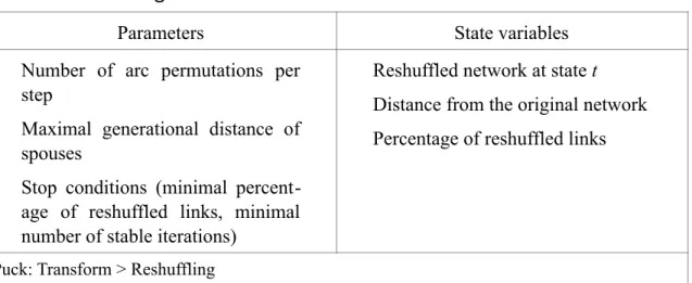
there-Table 5: Reshuffling Model

Parameters State variables Number of arc permutations per

step

Maximal generational distance of spouses

Stop conditions (minimal percent-age of reshuffled links, minimal number of stable iterations)

Reshuffled network at state t Distance from the original network Percentage of reshuffled links

fore have to re-transform P-graph arcs to single individuals or siblings according to a probability estimated from the mean fratry composition of the original network.

Once the network has been put into unimodal form, the procedure consists in swapping, at each iteration step, the target nodes of a selected set of arcs, subject to the constraints that gender-specific in- and out-degrees are conserved and that the genera-tional distance between the newly linked nodes in the original network must not exceed a certain maximal level. This local measure of generational distance—computed in an ego-centered manner from the numbers of ascending and descending arcs in the connecting chains—does not involve any global generational partition. Moreover, we impose the condition that no oriented cycles (and, a fortiori, no loops) should be formed—no node can become the descendant of a descendant or of itself.

This process is stopped as soon as a certain minimal percentage (which may be 100%) has been redistributed, and a certain maximal number of iterations have been run without augmenting the distance of the randomized from the original network.

Example: Testing the significance of Chimane consanguineous marriages

Let us apply this procedure to the Chimane dataset. As we are only interested in marriages, we first eliminate all unmarried individuals from the genealogy, thus reducing the number of parent-child links and, as a consequence, the constraints restricting the freedom of permutation. We then transform the Chimane-network into P-graph format and then repeatedly switch arcs (subject to the specified constraints) until 100% of all arcs have been reshuffled and 1000 iterations have been run without improving the dis-tance from the original network. Permutations of marriages shall only take place within a generation. The maximal distance thus achieved is about 43%. 13

Fig. 7 shows the reshuffeled network. Table 6 gives an overview of the changes the reshuffling process has brought about in the numbers of consanguine marriage cir-cuits (up to degree 3). As expected, the Chimane cross-cousin marriages clearly exceed the frequencies found in a reshuffled network, although the latter still exhibits a high per-centage of consanguineous marriages (7%, vs. 30% in the original network). However, the “Dravidian-type” structure has disappeared: parallel cousin marriages emerge, while some of the most preferred cross cousin marriages no longer show up at all. As con-firmed by the reshuffling test, the high frequency of cross cousin marriages in the Chi-mane network is not an artefact of demography or observer bias, but clearly indicative of other constraints—such as social norms—restricting matrimonial choice.

4.2. Alliance Networks: An Analytical Model

The case is quite different for alliance networks, whose simple structure as valued orient-ed graphs makes it possible to formulate an analytical solution for the problem of expect-ed circuit frequencies in reshufflexpect-ed networks (Roth et al., 2013). This is achievexpect-ed by con-structing a multinomial model on the alliance matrix whose parameters are limited to the total outgoing and incoming marriages for each group . We model this through a pair of 14

vectors k and k’ describing the numbers of incoming and outgoing marriage arcs for each group in the alliance network, such that each marriage goes to a cell ij of the random ma-trix with a probability proportional to kik’j. This formalism makes it possible to

analyti-Figure 7. Reshuffled Chimane Network (without single individuals). Reshuffled in

P-graph mode, 2 arc permutations per step, maximal generational distance 0, stop after 100% reshuffling and 1000 stable iterations. Graph distance from original 42.96%.

Table 6: Circuit Numbers Before and After Reshuffling*

Circuits Original Reshuffled Circuits Original Reshuffled Circuits Original Reshuffled

Z 0 6 FFBDD 29 3 FMBDD 0 1 FZ 1 0 FFZSD 50 3 FMZSD 0 2 FBD 0 13 FFZDD 0 3 FMZDD 23 0 FZD 93 3 MFBSD 27 6 MMB-SD 1 2 MBD 94 7 MFB-DD 0 1 MMB-DD 45 3 MZD 0 1 MFZSD 0 1 MMZS D 31 6 FZDD 2 0 MFZDD 53 1 FFBSD 0 3 FMBSD 45 6

* The original network is the Chimane genealogical network. Consanguineous circuits are listed up to degree 3.

cally express expectations of weights of the corresponding directed network, and, by ex-tension, the exact expectations of patterns of interest in the alliance network (Puck: [Group Network Window] > Analysis > Morphology). The problem has thus found an analytical solution, and simulation—while remaining useful for exploration and illustra-tion—is no longer required in order to determine the numbers of circuits (or other mor-phological indicators) which are to be expected if marriages were at random.

Example: expected connubial circuits in the Chimane alliance network

Table 7 shows the results of this model for the circuit frequencies in the alliance network of Chimane agnatic components. The salient features of this morphology—one single endogamous marriage (where one would have expected as many as 38), a number of dual circuits almost 4 times higher than expected, and an extremely low number of tri-angles (two percent of what would be expected)—clearly confirm the rules of a Dravidi-an marriage alliDravidi-ance system, which prohibits marriage both within one’s own group (loops) and with one’s allies’ allies (triangles), while favoring replication of marriages with established allies (dual circuits), without differentiation between wife-givers and wife-takers (reflected in the roughly equal surplus of cross and parallel circuits over their expected values).

5. Observer Bias Simulation (Virtual Fieldwork)

The second approach, virtual fieldwork (Hamberger and Gargiulo, 2014) consists in ex-plicitly simulating the data collection process, subject to the constraints of observer and informant behavior.

5.1. Genealogical Networks: Modeling Mobility and Memory Constraints

In our model (see Table 8), informants are successively chosen from a subset of the indi-viduals in the original network by an observer whose relative immobility is modeled by assigning preference weights to potential informants according to their kinship relation to the previous informant. This immobility may be interpreted socially (previous informants facilitate access to their relatives as subsequent informants) or spatially (related infor-mants live close together and are thus easier to reach). It is modeled by assigning higher weights to potential informants who are close to the current informant, where closeness

Table 7: Connubial Circuits in the Chimane Alliance Network

circuit type observed expected ratio observed/expected

loops 1 38.0 0.03 dual circuits 3534 844.3 4.19 parallel circuits 1850 461.0 4.01 cross circuits 1684 383.3 4.39 triangles 538 24418.2 0.02 transitive triangles 474 13502.9 0.04 cyclic triangles _{64 10915.3 0.01}

may be defined both quantitatively (by network distance) and qualitatively (by the type of kinship relation, e.g. agnatic, linear, and so on). In the simplest case, a constant weight > 1 is assigned to “close relatives”, while all others receive weight 1.

At each time step, the observer asks the informant to reveal his entire kinship en-vironment (as far as memory reaches) and then passes on to a different informant. The simulated network is thus gradually constructed as the sum of the memorized network environments of subsequently chosen informants. Each virtual "interview" consists in exploring the personal network of the informant by a (depth first) search process which recursively visits all direct neighbors (parents, spouses and children) of every visited node (starting with ego). We assume that informants share the same uniform memory ca-pacity, which we assume to decrease with genealogical distance from the informant at a given exponential rate smaller than one (the recall rate). The recall rate represents the 15

(constant) probability of recalling the relative of a recalled individual.

Example: distorting the balance of agnatic and uterine ancestor chains

As an example, let us look at the effects that an agnatically biased data collection would have on the Chimane dataset. Let us, for the purpose of illustration, assume that our network represents in miniature form the true morphology of the Chimane genealogy. As has been said, the Chimane have a cognatic kinship reckoning and an ambilocal resi-dence rule, which renders Daillant’s network largely balanced (although, even in this network, there is a moderate bias in favor of agnatic over uterine linear chains). Now as-sume that another observer explores this network, choosing his or her informants from the generational level G-2 (fortunately the Chimane dataset includes information on gen-erational levels in emic terms as ethnographic data, so we do not have to compute them). Fig. 8 and Table 9 show the effect that an increasing agnatic “inertia” of the ob-server—that is, a preference for choosing informants among the close agnates of previous informants—has, for increasing rates of genealogical recall, on the balance of agnatic and uterine linear chains (of length 3) in the network. We measure this balance as the surplus of persons for whom the agnatic great-grandfather is known over those for whom the

Table 8: Virtual Fieldwork Model for Genealogical Networks

Parameters State variables

Real network (number of individu-als, number and type of links, inci-dence of links and individuals) Subset of potential informants Observer inertia (preference for close informants) w

Informants (uniform) recall rate r Number of informants n

Actual informant at time t

Memorized subnetwork yielded by the informant at time t

Observed network at time t (which is the sum of all memorized sub-networks from 1 to t)

uterine great-grandmother is known, normalized by the number of persons for whom ei-ther the one or the oei-ther is known. In the real Chimane network, ei-there is a moderate ag-natic surplus of 9.8 percentage points.

As expected, the bias generally diminishes with improving recall rates. The effect of observer behavior, however, is not so clear-cut. Initially the redundancy of reconstruct-ed agnatic preconstruct-edigrees introducreconstruct-ed by an increasing propensity to stay within a group of close agnatic kin leads to higher rates of known agnatic ancestors and thus increases the agnatic bias. From a certain point onwards, however, the potential gains of this agnatic redundancy are exhausted, and further interviews add no more information to their own agnatic pedigree, while the observer’s preference for sticking to the same agnatic group

Figure 8. Surplus of agnatic over uterine linear chains (3 generations) (vertical axis)

for various preferences (weights) for agnatically (maximal chain length: 6) related informants (left depth axis) and recall rates (right depth axis). Based on 100 runs.

prevents him or her from exploring the pedigree of other agnatic groups, thus reducing the agnatic bias of the network.

This non-linear effect of observer bias characterizes not only its impact on linear chains, but also on cousin relations and on cousin marriages, whose ratio may be affected both in a positive and in a negative way, depending on the overall genealogical memory. This is bad news for comparative anthropology, for it means that neither absolute circuit frequencies nor closure rates (percentages of kinship chains that link spouses) can serve as an unbiased indicator of matrimonial preferences.

5.2. Alliance Networks: Modeling Observer “Endogamy”

The model for alliance networks (see Table 10) shares the basic properties of the model for genealogical networks, with the difference that informants are now groups (rather than individuals), which we assume to be equally accessible as informants and to have perfect memory of their members’ marriages. Contrary to the case of genealogical net-works, the length of the interview now forms part of the observer’s choice to stay with the same group or to pass to the next one after each single bit of information (that is, each revealed marriage link). Accordingly, the duration of the virtual fieldwork process is now limited by the predetermined number of searched marriage links rather than by the prede-termined number of informants.

Again, we assume the observer to be constrained by social or spatial immobility, which we now can model simply as a preference for (or aversion against) staying with the same group (in other words, choosing the informants with a network distance of zero to the previous informant group). In addition, the observer may show a preference for (or aversion against) following a “snowballing” process and visiting the groups named as

Table 9: Agnatic Bias Variations in Virtual Fieldwork*

*Surplus of agnatic over uterine linear chains (3 generations) in virtually “observed” Chimane genealogy for various preferences (weights) for agnatically (maximal chain length 6) related informants (columns) and recall rates (rows).

allies by previous informant groups (that is, groups at a network distance of 1). The re-construction of alliance networks by the virtual fieldwork process thus follows a process that is structurally similar to the generation of alliance networks as such (see Section 2.2); the difference being that the random selection weighted according to network distance now characterizes the choice of informants and not of marriage partners: social or spatial immobility thus corresponds to endogamy, snowballing to relinking, and so on.

Example: the effects of observer immobility on the over- or underestimation of circuits

To illustrate the method, we shall examine the effect of different combinations of observer inertia and snowballing behavior on the number of observed dual circuits (mar-riage redoubling or exchange configurations) in an alliance network, as compared with their number in the real network. The diagram on the left in Fig. 9 shows the results for the Chimane alliance network of agnatic components; the one on the right for the alliance network we have simulated in Section 2.2, starting from the same number of groups and marriages, by applying a weight for marriage redoublings that corresponds to the Chi-mane rules.

In both cases, increasing inertia tends to increase the normalized number of dual circuits observed in the alliance network due to the concentration of observed marriages in the environment of the observer, which gives relinking marriages a greater chance of being observed. The effects of snowballing are somewhat more ambiguous. It clearly tends to augment the number of dual circuits as long as observer inertia is relatively low, since it keeps the mobile observer within a cluster of strongly interconnected nodes, but it may also mitigate the overestimation of circuits for high values of observer inertia, by pushing the observer to move from one node to another.

Table 10: Virtual Fieldwork Model for Alliance Networks

Parameters State variables Real network (number of groups,

number of links, incidence of links and groups)

Observer’s informant choice pref-erences (inertia w1 and snowballing

w2)

Number of links to be observed n

Actual informant group at time t Marriage link and partner group revealed by the informant group at time t

Set of potential informant groups (whose marriage links have not yet been totally revealed)

Observed network at time t (made up of all groups and links revealed from 1 to t)

However, while changes in observer behavior appear to operate roughly in the same direction for both cases, they operate on quite different levels: in the case of the true Chimane network, the number of dual circuits is generally largely underestimated, and a strong local immobility and/or snowballing strategy is required to approach their true values. In the case of the simulated network, on the contrary, the numbers of dual circuits are roughly correctly estimated by the neutral observer, while observer immobility as well as snowballing lead to their overestimation. This is due to the fact, noted in Section 2.2, that the simulated network is locally homogenous—all nodes being structurally simi-lar, even if there are large differences between node-pairs—while in the true Chimane network, marriages are concentrated in the proximity of a large main component, so that the observer has to stick to this component and its environment in order to record the cir-cuits of the network. The (distorting or elucidating) effect of local in-depth studies de-pends crucially on the homogeneity or heterogeneity of the social environment.

6. Conclusion

The various simulation techniques presented in this paper serve a variety of different pur-poses. Some of them, such as the straightforward agent-based simulation techniques and the virtual fieldwork models, are first and foremost exploratory and experimental tools destined to get a clear idea of the impact of a factor (or combination of factors) on the morphological properties of kinship networks in general—insights which may then guide the interpretation of empirical networks. Other techniques, such as the automatic rule dis-covery or the reshuffling models, are instruments to examine the morphology of concrete

Figure 9. Effects of observer inertia (right depth axis) and snowballing (left depth axis)

on the over- or underestimation of the normalized number of dual circuits (vertical axis), for the Chimane alliance network (left) and the simulated homogenous alliance network (right). 10% of arcs explored. Based on 100 runs.

empirical networks by focusing on the rules that may have brought them about, or the degree to which they may be due to chance.

Most of these methods are not restricted to the domain of kinship. They are ap-plicable to all kinds of social networks in which past (direct or indirect) links between agents are supposed to promote or hamper the formation of future links, and where the exploration of the network by observers is likely to follow certain types of links at the cost of following other types of links. Thus, meta-modeling techniques advance the state of the art in the discovery of generative models for complex networks. For example, Menezes and Roth (2014) propose explanatory generative models for a simple brain, an Internet social network and a network of protein interactions. The multinomial model for calculating expected morphological indicators of alliance networks is equally applicable to networks of migration flows or international trade. The virtual fieldwork model can be generalized to other types of search processes, such as net mining algorithms (see Gargiu-lo and Roth 2013).

All of the models we have presented should be viewed as methodologies open to further development. Their value mainly consists in being exploratory and critical tools. They serve to grasp the horizon of potential causes of kinship network phenomena, and to scrutinize the validity of (theoretical or emic) models claiming to render account of these phenomena. Rather than furnishing ready-made keys to the interpretation of empirical kinship networks, they help improve our insight into the complexity of network-generat-ing processes, and to make us skeptical regardnetwork-generat-ing any theory postulatnetwork-generat-ing a one-to-one re-lationship between network phenomena and behavioral rules. As our experiments have shown, many behavioral parameters have non-linear effects on morphological indicators. These effects are, moreover, often contingent on the presence or absence of other mor-phological traits. This does not mean that the factors underlying the generation of kinship networks are too complex to be analyzed. However, their analysis depends crucially on the availability of data permitting us to get a handle on this complexity; that is, on having access to precise, comprehensive and transparent ethnographies. Computer simulation reminds us, ultimately, of the vital importance of rigorous qualitative research.

References

Albert, R. and A.-L. Barabási. 2002. Statistical mechanics of complex networks. Reviews

of Modern Physics 74: 47–97.

Batagelj, V. and A. Mrvar. 2008. Analysis of kinship relations with Pajek. Social Science

Computer Review 26(2): 224–46, http://ssc.sagepub.com/ cgi/content/abstract/

26/2/224.

Black, S. 1978. “Polynesian outliers. A study in the survival of small populations,” in

Simulation Studies in Archeology. Edited by I. Hodder, pp. 63-76. Cambridge:

Cambridge University Press.

Christiansen, J. H. and M. R. Altaweel. 2005. Understanding Ancient Societies: A New

Approach Using Agent-Based Holistic Modeling, Structure and Dynamics, Social Dynamics and Complexity. Institute for Mathematical Behavioral Sciences, http://

escholarship.org/uc/item/33w3s07r

Daillant, I. 2003. Sens dessus dessous. Organisation sociale et spatiale des Chimane

d’Amazonie bolivienne. Nanterre: Société d’ethnologie.

Dyke, B. 1981. Computer simulation in anthropology. Annual Review of Anthropology 10, 193-207.

Fischer, M. D. 1986. Expert systems and anthropological analysis. Bulletin of

Informa-tion in Computing and Anthropology 4:1-4.

______ 2004. Applications in Computing for Social Anthropologists. London: Routledge. ______ 2006. The ideation and instantiation of arranging marriage within an urban

com-munity in Pakistan, 1982-2000. Contemporary South Asia 15(3): 325-339.

Fischer, M. D. and D. B. Kronenfeld. 2011. “Simulation (and modeling),” in A

Compan-ion to Cognitive Anthropology. Edited by D. B. Kronenfeld, G. Bennardo,V. C. de

Munck, M. D. Fischer, pp. 210-226. London: Wiley-Blackwell.

Gargiulo, F. and C. Roth. 2013. Exploration bias when sampling weighted networks. Poster at the 4th _{Workshop on Complex Networks, Berlin, March 2013 (13-15).}

Geller, A., J. F. Harrison and M. Revelle. 2011. Growing social structure: An empirical multiagent excursion into kinship in rural North-West Frontier Province. Structure

and Dynamics 5(1), 3, http://www.escholarship.org/uc/item/4ww6x6gm.

Gilbert, J. P. and E. Hammel. 1966. Computer simulation and analysis of problems in kinship and social structure. American Anthropologist 68: 71–93.

Hamberger, K. and F. Gargiulo. 2014. Virtual fieldwork. Modeling observer bias in kin-ship and alliance networks. Journal of Artificial Society and Social Simulation 17 (3) 2, http://jasss.soc.surrey.ac.uk/17/3/2.html.

Hamberger, K., C. Grange, M. Houseman and C. Momon. 2014. Scanning for patterns of relationship: Analyzing kinship and marriage networks with Puck 2.0. History of

the Family 19 (4): 564-596.

Hamberger, K., M. Houseman and D. R. White. 2011. “Kinship network analysis,” in The

Sage Handbook of Social Network Analysis. Edited by P. Carrington and J. Scott,