Clustering weather types for urban outdoor
thermal comfort evaluation in a tropical area
The MIT Faculty has made this article openly available.
Please share
how this access benefits you. Your story matters.
Citation
Acero, Juan A. et al. "Clustering weather types for urban outdoor
thermal comfort evaluation in a tropical area." Theoretical and
Applied Climatology 139, 1-2 (September 2019): 659–675. © 2019
Springer-Verlag
As Published
https://doi.org/10.1007/s00704-019-02992-9
Publisher
Springer Science and Business Media LLC
Version
Author's final manuscript
Citable link
https://hdl.handle.net/1721.1/128526
Terms of Use
Creative Commons Attribution-Noncommercial-Share Alike
Clustering weather types for urban outdoor thermal comfort evaluation in a
tropical area
Cite this article as: Juan A. Acero, Elliot J. K. Koh, Gloria Pignatta, Leslie K. Norford, Clustering
weather types for urban outdoor thermal comfort evaluation in a tropical area, Theoretical and Applied
Climatology, doi: 10.1007/s00704-019-02992-9
This Author Accepted Manuscript is a PDF file of a an unedited peer-reviewed manuscript that has been accepted for publication but has not been copyedited or corrected. The official version of record that is published in the journal is kept up to date and so may therefore differ from this version.
Terms of use and reuse: academic research for non-commercial purposes, see here for full terms.
Clustering weather types for urban outdoor thermal comfort evaluation in a tropical area
Juan A. Acero*1, Elliot J. K. Koh1, Gloria Pignatta1, Leslie K. Norford2
1 CENSAM, Singapore-MIT Aliance for Reasearch and Tecnology (SMART), 1 Create Way, #09-03, Singapore
138602
2
Department of Architecture, Massachusetts Institute of Tecnology (MIT), 265 Massachusetts Ave, MA 02139, USA
*Corresponding author: juanangel@smart.mit.edu; Tel. +65 6516 6129; ORCID: 0000 0001 6214 0605
Abstract
Outdoor thermal comfort is a major concern in urban areas throughout the world. Sophisticated modelling techniques have been developed to analyze the interaction of the urban areas with the regional climate. However, in most cases, the assessment of outdoor thermal comfort is not based on a long term analysis and provides results only for specific meteorological conditions. In this study, we apply a clustering method to yearly weather files with the aim of obtaining representative boundary conditions for urban microclimatic models. The results describe typical-day weather situations commonly known as weather types. The study is carried out in the hot and humid tropical conditions of Singapore, where ten weather types are defined. The analysis of the clusters’ performance shows adequate results. ENVI-met (v.4.3) model is used to evaluate the impact of weather types on thermal comfort in a courtyard surrounded by high-rise buildings. Results not only show different levels of thermal comfort but also different spatial distribution and diurnal evolution inside the courtyard for each weather type. We conclude that it is relevant to analyze thermal comfort in all predominant weather conditions so as to have an accurate and complete assessment of the existing thermal situation. The approach presented in this study will provide better support to planners and decision makers in the development of urban spaces in regard to their expected use.
Highlights
k-means clustering method is reliable to develop weather types for thermal comfort assessment
Ten weather types were developed for a specific area of Singapore
Using weather types is relevant and improves for thermal comfort evaluations
Keywords
1. Introduction
During the last decade the topic of outdoor thermal comfort has become a priority to attain sustainable and livable cities (Chen and Ng 2012; Emmanuel 2016). One of the reasons is the global increase of air temperature due to climate change and the other is the influence of the urban heat island (UHI). On the whole urban areas present different climatic characteristics than nearby rural areas (Stewart and Oke 2012) that affect the outdoor thermal comfort.
Different urban developments and urban designs have different impact on local thermal comfort
depending on the influence of regional climate and the surrounding land use. Generally, urban areas tend to increase air temperature due to accumulation of heat, reduce humidity due to a decrease of vegetative elements and pervious grounds, and slow the mean air flow in the urban area due to the increase of surface roughness caused by buildings and urban elements of different heights (Oke 1987).
Many studies have analyzed strategies and measures to improve urban thermal comfort focusing on materials (Santamouris et al. 2011; Erell et al. 2014; Taleghani and Berardi 2016); vegetation (Ng et al. 2012; Tan et al. 2014; Lobaccaro and Acero 2015; Zölch et al. 2016; Besir and Cuce 2018); ventilation (Ali-Toudert and Mayer 2006; Ng 2009; Krüger et al. 2011; Ignatius et al. 2015; Hong and Lin 2015) and water bodies (Nishimura et al. 1998; Shashua-bar et al. 2009; Steeneveld et al. 2014). The impact of these can be assessed by means of measurements and/or modelling (Gulyás et al. 2006; Chow et al. 2011; Zölch et al. 2016). Reliable results are obtained from the former but the costs in terms of time and resources are significant. Additionally, the evaluation of certain mitigation measures, individually or combination, cannot always be undertaken with measurements, especially if they are not yet implemented. Numerical modelling can overcome these limitations despite a certain level of inaccuracy in the results that must be assumed (Acero and Herranz-Pascual 2015).
In the case of numerical modelling of thermal comfort, different tools/approaches that combine
computational fluid dynamic models with radiative models can be used, e.g. ENVI-met (Bruse and Fleer 1998) and OpenFOAM (Weller et al. 1998). All of these require significant computing power and can take a huge amount of time to perform their calculations especially if they are to provide results during a representative period of time (e.g. more than one year). Thus, to shorten the amount of calculations, most of the studies select specific weather conditions (many times based on measured data) to evaluate their impact on thermal comfort. However, these do not represent all the weather conditions and thus cannot always provide reliable results when assessing thermal comfort on an annual basis. In this sense, the real impact of mitigation measures can be misleading or incomplete. Actually, most of the studies carried out consider only one or perhaps a few meteorological conditions (Ketterer and Matzarakis 2014; Müller et al. 2014; Taleghani et al. 2015; Morakinyo et al. 2017).
Weather patterns have been used to identify relationships between the synoptic scale atmospheric circulations and local scale meteorological impacts such as air quality (Demuzere and van Lipzig 2010), and urban climate (Morris and Simmonds 2000; Hidalgo et al. 2014). Also, they are used to dynamically downscale broader scale atmospheric models (Pinto et al. 2010) to higher resolution scales, especially for climate change impact scenarios (Hoffmann and Heinke SchlüNzen 2013; Hidalgo et al. 2014).
One of the most commonly used methods to classify weather types is the cluster analysis, especially the k-means-based method (Huth et al. 2008). Although there are other methods (e.g
artificial-neural-network-based), the former seems to perform well. Recently, Hidalgo and Jougla (2018) have applied the Partitioning Around Medoids (PAM) method to an urban climate study in Toulouse (France).
In this study, we present a new approach for the annual evaluation of outdoor thermal comfort based on the use of weather types. Specifically, they have been obtained to be used as boundary conditions of a microscale model (ENVI-met). The overall impact of the weather types is compared with individual conditions showing the relevance of using a set of representative weather conditions for annual outdoor thermal comfort assessments.
2. Methods
2.1 Study area and regional climate
The study has been developed in Singapore, an island located at the southern end of the Malayan Peninsula (1˚N, 104˚E) with an approximate land area of 712 km2
and a population of 5.6 million inhabitants in 2016 (Singapore Department of Statistics 2017).
The climate in Singapore is classified as tropical rainforest (Koppen climate classification Af). Typically, high and uniform air temperatures together with high humidity occur throughout the year. The annual mean temperature is ~27.5 ˚C with minor monthly variation (< 2 ˚C). The hottest months are April and May, due to light winds and strong sunshine. The diurnal temperature range is relatively small (~7 ˚C). The daily maximum temperature is 31-33 ˚C while the minimum temperature is 23-25 ˚C. Relative humidity varies from 90% in the morning (before sunrise) to 60% in the afternoon (when no rain). In periods of rain, values can reach 100% and the annual average is 84%. Annual total precipitation is high, reaching ~2190 mm (Roth and Chow 2012).
Annual variations in regional climate caused by the Asian monsoon affect cloudiness, surface wind speed, and wind direction (Chow and Roth 2006). Higher surface wind speeds occur from November to February and are consistent with winds from the Northeast between December and March (NE monsoon season). However, between May and September surface winds are generally from South to Southeast (SE monsoon season). These two seasons are separated by two Inter-monsoon seasons characterized by variable wind direction and light winds (Meteorological Service Singapore 2016). During these periods, sea breezes can frequently be developed and the urban heat island phenomenon has more emphasis (Li and Norford 2016). Although precipitation occurs during all the year (i.e. no clearly defined wet and dry season), higher levels occur in the first months of the NE monsoon season (i.e. December and January).
Due to its location close to the equator, cloudiness in Singapore is high, and completely covered or mostly covered skies are frequent (Meteorological Service Singapore 2016).
Inside Singapore we have selected a courtyard between high-rise buildings where we have tested and evaluated our approach for thermal comfort assessment (see section 2.2). Courtyards are usually designed by the Singapore Housing Development Board (HDB) to be used for outdoor activities. Our study area is located in Punggol in the northern part of the island (Fig. 1).
Fig. 1 Location of the study area in Singapore and the morphology of the analyzed courtyard in between
high-rise buildings
2.2 Development of weather types
2.2.1 Data
In order to define weather types (WT) that describe the representative meteorological conditions close to the surface, hourly data of air temperature (Ta), relative humidity (RH), wind speed (WS) and direction (WD), and Solar Radiation (SolRad) have been used. The first four climate variables were selected from the meteorological station of Seletar and the last one was taken from Changi Airport. Both belong to the National Environmental Agency (NEA) of Singapore (Fig. 1).
For the calculation of WTs (see section 2.2.3), data of year 2016 were used. Only days with data available at least 75% of the time were selected (i.e. 336 days, 92% of the total).
2.2.2 Clustering method
The statistical k-means method has been applied to define clusters that represent the characteristics of the weather conditions of our study area. Previous studies (Beck and Philipp 2010; Hidalgo et al. 2014) suggest that this method is reliable for defining WTs (Hoffmann and Heinke SchlüNzen 2013).
The k-means method is based on calculating the squared Euclidean distance (SED) between two data objects that can include one or more variables. In an interactive process, the algorithm looks for the minimum value of the so called ‘within-cluster sum of squares (WSS)’ (Hoffmann and Heinke SchlüNzen 2013) that is defined as the sum of the squared differences between the observations and the
corresponding centroid:
𝑊𝑆𝑆 = ∑ ∑ ‖𝑥 − 𝑧𝑖‖2 𝑥∈𝐶𝑖
𝑘
𝑖=1
where x denotes all the data belonging to the cluster Ci; zi is the ith corresponding cluster centroid (CC)
and k is the number of clusters.
The iteration process starts with the selection of cluster centroids (CC). The SED is calculated for each combination of CC and data objects. All data objects are assigned to their nearest CC to form the cluster. Data objects of each cluster are averaged to provide a new CC. This procedure of CC reassignment and calculation of SED ends when no data needs to be reassigned to another CC. Thus, data objects are grouped with respect to their similarity. The final CC are unique values of the considered variables that represent the data objects in the clusters.
The outcome provided by the k-means algorithm depends on the initial selection of CC. Thus, to minimize deviation we have run the k-means algorithm 5000 times and selected the CC with the lowest WSS.
For the selection of the optimal number of clusters (i.e. weather types) in which our data should be divided, we have used the dynamic validity Index (DVIndex) developed by Shen et al. (2005). This index manages to balance in an effective way the compactness and the separateness of the clusters. With a higher number of clusters, the intracluster compactness increases while the intercluster separation
decreases. To achieve the optimal number of clusters, the sum of compactness and separation should be at a minimum.
𝐷𝑉𝐼𝑛𝑑𝑒𝑥(𝑘) = 𝐼𝑛𝑡𝑟𝑎𝑅𝑎𝑡𝑖𝑜(𝑘) + 𝛾 ∙ 𝐼𝑛𝑡𝑒𝑟𝑅𝑎𝑡𝑖𝑜(𝑘) where 𝐼𝑛𝑡𝑟𝑎𝑅𝑎𝑡𝑖𝑜(𝑘) = 𝐼𝑛𝑡𝑟𝑎(𝑘) 𝑀𝑎𝑥𝐼𝑛𝑡𝑟𝑎 𝐼𝑛𝑡𝑒𝑟𝑅𝑎𝑡𝑖𝑜(𝑘) = 𝐼𝑛𝑡𝑒𝑟(𝑘) 𝑀𝑎𝑥𝐼𝑛𝑡𝑒𝑟 𝐼𝑛𝑡𝑟𝑎(𝑘) = 1 𝑁∙ ∑ ∑ ‖𝑥 − 𝑧𝑖‖ 2 𝑥∈𝐶𝑖 𝑘 𝑖=1 𝑀𝑎𝑥𝐼𝑛𝑡𝑟𝑎 = max 𝑖=1,…,𝐾(𝐼𝑛𝑡𝑟𝑎(𝑖)) 𝐼𝑛𝑡𝑒𝑟(𝑘) = 𝑀𝑎𝑥𝑖,𝑗(‖𝑧𝑖− 𝑧𝑗‖ 2 ) 𝑀𝑖𝑛𝑖≠𝑗(‖𝑧𝑖− 𝑧𝑗‖ 2 )∙ ∑ ( 1 ∑ (‖𝑧𝑖− 𝑧𝑗‖ 2 ) 𝑘 𝑗=1 ) 𝑘 𝑖=1 𝑀𝑎𝑥𝐼𝑛𝑡𝑒𝑟 = max 𝑖=1,…,𝐾(𝐼𝑛𝑡𝑒𝑟(𝑖))
where N is the number of data objects to be clustered, K is the pre-defined upper bound number of clusters (20 in our case), zi is the CC of the cluster Ci, and ϒ is a tuning parameter.
Following Hoffmann and Heinke SchlüNzen (2013), ϒ was assigned a value of 0.5.
2.2.3 Procedure for cluster calculations
With the aim of representing daily weather patterns (i.e. daily mean cycles) we have defined the cluster structure using the following variables: daily mean temperature, daily temperature amplitude, daily mean vapour pressure, daily mean global radiation, and mean u – v wind components.
The selected variables were suitable to analyze outdoor thermal comfort in the context of the Singapore climate. Similar variables were used by Hidalgo et al. (2014).
After applying the clustering method (see section 2.2.2) to the previous variables, each day was assigned to a specific cluster and thus was associated with others with similar climatic features. For each cluster of days a diurnal mean cycle was calculated to represent the climatic variability for that specific WT. Hourly series for Ta and RH were obtained by averaging data in each cluster.
Although the clustering method was initially applied independently to different seasons of the year (NE monsoon, SE monsoon and Inter-monsoon), the final clusters (i.e. WTs) were calculated with a unique annual dataset. In the climate context of Singapore, with small annual variations in weather variables (see section 2.1), this is a valid approach that can reduce the total number of WTs and thus reduce the outdoor thermal comfort conditions to be assessed in our study area (see section 2.3).
2.3 Modelling the impact of outdoor thermal comfort
To evaluate the impact of WTs on thermal comfort we have used ENVI-met model (see section 2.3.1). Climatic outputs of the model (Ta, RH, mean radiant temperature (Tmrt) and WS) were used to calculate the Physiological Equivalent Temperature (PET) (Höppe 1999) on an hourly basis. The human metabolic
rate and other human parameters were standardized (age: 35 years; height: 1.74 m.; metabolic rate: 80 w/m2; clothing: 0.9; weight:75 kg; sex: male).
2.3.1 Description of ENVI-met model
This is a well-known and extended used model that is frequently applied to analyze the impact of the urban environment on the microclimate and thermal comfort (Krüger et al. 2011; Ng et al. 2012; Müller et al. 2014; Jänicke et al. 2015; Lobaccaro and Acero 2015; Yang et al. 2015, 2016; Taleghani and Berardi 2016; Morakinyo et al. 2017). The model simulates surface-plant-atmosphere interactions with a spatial resolution between 0.5 to 10 meters. Air flow is solved with the standard k-ɛ turbulence closure model for the Reynold Average Navier-Stokes (RANS) equations. The model considers a complete radiation budget (i.e. direct, reflected and diffused solar radiation and longwave radiation). However, certain
approximations are included (Huttner 2012) that need to be taken into account during the assessment of the results. The performance of the model has been evaluated in several studies (Chow et al. 2011; Yang et al. 2013; Jänicke et al. 2015; Acero and Arrizabalaga 2018)
Version 4.3 of ENVI-met allows forcing climate variables along the simulation to account for the variation of meteorological variables along the day. However, only boundary conditions of Ta and RH can be updated during the diurnal simulation. WS and WD as well as cloudiness remain constant.
Initial conditions of soil moisture and temperature are also input values required by ENVI-met.
Especially, initial soil moisture is an extremely sensitive parameter if unsealed surfaces are present to a notable degree in the model domain due to their limitation to provide sufficient water for evaporation (Bruse, person. comm.). On the contrary, initial soil temperature is a less sensitive variable because it can quickly adjust to the calculated conditions. A sensitivity study carried out by Roth and Lim (2017) in Singapore showed the importance of the initial soil moisture in predicting air temperature when conditions become too dry.
2.3.2 Model setup
The spatial domain of the model has been extended further away of the limits of the courtyard (our study area) to consider the influence of the surrounding urban elements. Although version 4.3 of ENVI-met has no limitations in the model size, a compromise between size of model domain, resolution and
computation time has to be met. In our study, a 3 x 3 m horizontal resolution has been selected. On the vertical, the grid size was 2 m in the five lowest levels (i.e. up to 10 m. a.g.l.). From this height upwards the grid increased the vertical resolution with a telescoping factor of 18%. The model domain covered a horizontal area of 399 x 414 m (i.e. 133 x 138 grid cells) and extended in the vertical to 122 m (i.e. 20 grid cells).
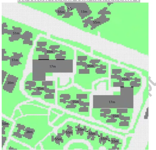
Characteristics of the spatial configuration of the model are presented in Fig. 2. The precise location of the buildings was obtained from OpenStreetMap. Height of each building was estimated considering 3 m per floor except for the ground floor that 4 m height was assumed. The range of building heights within the spatial domain was 13-55 m. In particular, the six residential towers that are located around the courtyard (our study area) are 55 m high and the two smaller buildings (carparks) are approximately 17 m. The buildings envelope (i.e. walls and roofs) has been modeled with a unique material (i.e. concrete slab), for which precise properties can be seen in Table 1. The model included the existing grass (10 cm high), and the rest of the ground surface was covered with a red brick road, concrete pavement and traditional black asphalt road.
Fig. 2 Modelled spatial domain including building footprint and height, and vegetation (grass) Table 1 Characteristics of the assigned
material for the building envelope
Building material description (walls & roofs) Description Concrete slab
(hollow block) Thickness [m] 0.30 Thermal Conductivity (W/m2K) 0.86 Albedo 0.30 Emissivity 0.90 Specific heat (J/kgºC) 840
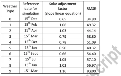
Meteorological conditions were extracted from weather stations at Seletar and Changi (Fig. 1). These were clustered in ten representative WTs following the methodology presented in section 2.2. Ta and RH were considered on an hourly basis and the rest of the meteorological conditions remained constant during the simulation (i.e. WS, WD, and Cloud Cover). For each WT, model estimation of solar radiation was adjusted by comparing hourly direct and diffuse shortwave radiation estimations in the absence of buildings with the clustered diurnal cycle of solar radiation. A linear regression analysis of the pairs of solar radiation data (clustered & ENVI-met estimations) was performed. For each WT, an adjustment factor (slope of the linear equation with constant value equal to 0) was obtained. Considering this correction, the RMSE of ENVI-met hourly solar radiation estimations with respect to clustered diurnal cycle data ranged for the different WTs between 34.9 to 83.0 Watt/m2 (Table 2).
Table 2 ENVI-met solar adjustment factor for each weather type, and
RMSE of the hourly incoming solar radiation estimations
Weather Type Reference date for simulation Solar adjustment factor (slope linear equation)
RMSE 0 15th Dec 0.65 34.90 1 15th Feb 1.06 49.32 2 15th Apr 1.03 44.14 3 15th Mar 0.79 58.80 4 15th Oct 0.78 51.09 5 15th Jan 0.50 40.32 6 15th Sept 0.66 54.40 7 15th Jul 1.05 57.10 8 15th Jun 1.02 56.97 9 15th Mar 1.16 83.00
Due to the sensitivity of the model to soil conditions (see section 2.3.1), specific data for Singapore were used. For each WT, mean monthly values of soil temperature where extracted from Changi
(Meteorological Service of Singapore 2017) and soil moisture values were taken from measured data in Singapore reported by Roth and Lim (2017).
Table 3 summarizes the meteorological and soil input parameters for ENVI-met
The simulations were launched at 4:00 LAT (Local Apparent Time, GMT+7), approximately 2 hours before sunrise, and run for 40 hours. Outputs of the model were analyzed for the last 24 hours of simulation (i.e. a complete diurnal cycle) so as to guarantee a suitable spin-up of the model.
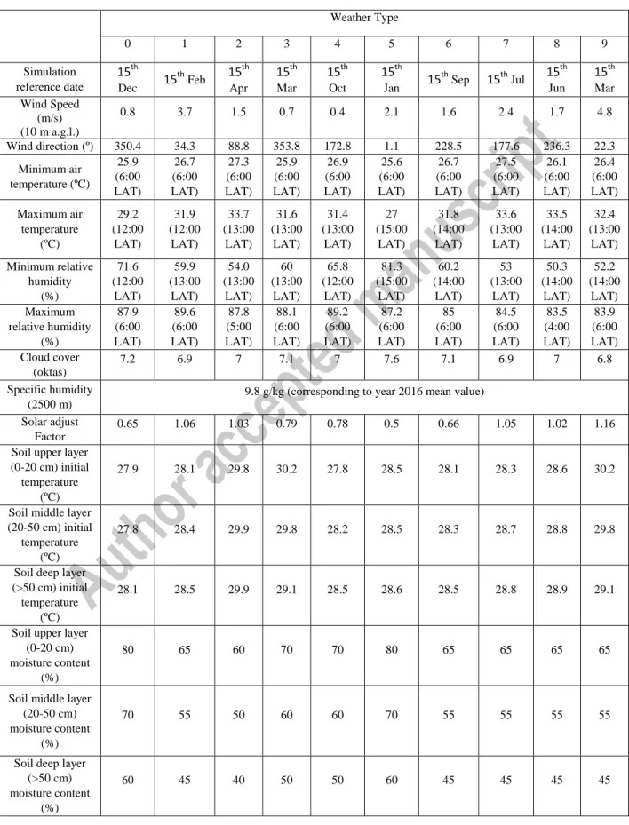
Table 3 Description of the model meteorological boundary configuration of each weather type. Wind
speed, wind direction, air temperature, relative humidity and cloud cover values are output from the clustering procedure (see section 3.2 and 3.3), specific humidity (2500 m) is from US-NCEP data and the soil temperature and moisture is from Roth and Lim (2017).
Weather Type 0 1 2 3 4 5 6 7 8 9 Simulation reference date 15th Dec 15 th Feb 15 th Apr 15th Mar 15th Oct 15th Jan 15 th Sep 15th Jul 15 th Jun 15th Mar Wind Speed (m/s) (10 m a.g.l.) 0.8 3.7 1.5 0.7 0.4 2.1 1.6 2.4 1.7 4.8 Wind direction (º) 350.4 34.3 88.8 353.8 172.8 1.1 228.5 177.6 236.3 22.3 Minimum air temperature (ºC) 25.9 (6:00 LAT) 26.7 (6:00 LAT) 27.3 (6:00 LAT) 25.9 (6:00 LAT) 26.9 (6:00 LAT) 25.6 (6:00 LAT) 26.7 (6:00 LAT) 27.5 (6:00 LAT) 26.1 (6:00 LAT) 26.4 (6:00 LAT) Maximum air temperature (ºC) 29.2 (12:00 LAT) 31.9 (12:00 LAT) 33.7 (13:00 LAT) 31.6 (13:00 LAT) 31.4 (13:00 LAT) 27 (15:00 LAT) 31.8 (14:00 LAT) 33.6 (13:00 LAT) 33.5 (14:00 LAT) 32.4 (13:00 LAT) Minimum relative humidity (%) 71.6 (12:00 LAT) 59.9 (13:00 LAT) 54.0 (13:00 LAT) 60 (13:00 LAT) 65.8 (12:00 LAT) 81.3 (15:00 LAT) 60.2 (14:00 LAT) 53 (13:00 LAT) 50.3 (14:00 LAT) 52.2 (14:00 LAT) Maximum relative humidity (%) 87.9 (6:00 LAT) 89.6 (6:00 LAT) 87.8 (5:00 LAT) 88.1 (6:00 LAT) 89.2 (6:00 LAT) 87.2 (6:00 LAT) 85 (6:00 LAT) 84.5 (6:00 LAT) 83.5 (4:00 LAT) 83.9 (6:00 LAT) Cloud cover (oktas) 7.2 6.9 7 7.1 7 7.6 7.1 6.9 7 6.8 Specific humidity (2500 m)
9.8 g/kg (corresponding to year 2016 mean value) Solar adjust
Factor
0.65 1.06 1.03 0.79 0.78 0.5 0.66 1.05 1.02 1.16
Soil upper layer (0-20 cm) initial temperature
(ºC)
27.9 28.1 29.8 30.2 27.8 28.5 28.1 28.3 28.6 30.2
Soil middle layer (20-50 cm) initial
temperature (ºC)
27.8 28.4 29.9 29.8 28.2 28.5 28.3 28.7 28.8 29.8
Soil deep layer (>50 cm) initial temperature
(ºC)
28.1 28.5 29.9 29.1 28.5 28.6 28.5 28.8 28.9 29.1
Soil upper layer (0-20 cm) moisture content
(%)
80 65 60 70 70 80 65 65 65 65
Soil middle layer (20-50 cm) moisture content
(%)
70 55 50 60 60 70 55 55 55 55
Soil deep layer (>50 cm) moisture content
(%)
2.4 Impact assessment of weather types
To evaluate the influence of WTs in the overall thermal environment, results of ENVI-met were analyzed at five moments of the day: 9 h., 12 h., 15 h., 18 h., 21 h. (LT: GMT+8). Output values of Ta, RH, WS, Tmrt and PET at 1 m. a.g.l. were extracted and analyzed in the whole courtyard area.
The results of the different WTs were integrated to provide weighted mean values of the climate output variables (Ta, RH, WS, Tmrt) at each space (grid cell) of the courtyard. The contribution of each WT to the weighted mean values corresponds to its frequency of occurrence during the year. Thus, at each hour, weighted mean values of Ta, RH, WS and Tmrt were calculated as:
𝑣𝑎𝑟
𝑤= ∑ 𝑓
𝑖 𝑘𝑖=1
∙ 𝑣𝑎𝑟
𝑖where varw is the weighted mean value of a climate variable at a specific hour; fi is the frequency of
occurrence of each WT along the year; vari is the value of a climate variable at a specific hour for WT i; and k is the total number of WTs.
A quantitative analysis of the output values of the model (Ta, RH, WS, Tmrt) identified the difference between the results of individual WTs and the weighted mean values (integrating all WTs).
In the case of thermal comfort, a spatial analysis of PET determined the variation of percentage of the courtyard area that meets the neutral thermal comfort range. As defined by Heng and Chow (2019) acceptable levels of thermal comfort in Singapore are in the PET range of 21.6 ⁰ C to 31.6 ⁰ C. PET was calculated on an hourly basis in each grid cell of the 10 individual WTs. The assessment was based on the comparison of individual WTs with the whole set of WTs considering the percentage of occurrence during the year. In the last case, it was considered that a grid cell met the acceptable thermal comfort range when it was met in all the individual WTs during the year.
3. Results and discussion
3.1 Performance of the clustering procedure
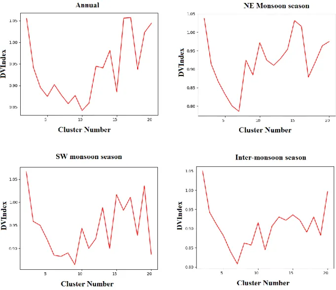
Fig. 3 shows the DVIndex (see section 2.2.2) for different numbers of clusters. Calculations were made for the annual dataset (336 days) and also for different seasons: NE monsoon (120 days in December, January, February and March), SW monsoon (106 days in June, July, August and September) and Inter-monsoon season (110 days in April, May, October and November). For these cases, the minimum DVIndex value corresponds to 10, 7, 9 and 7 clusters, respectively.
Quantitative measures of the performance of the clustering procedure are presented in Table 4. These represent how the measured hourly data is represented by the clustered hourly results. Calculations made for different datasets (i.e. annual and three seasons independently) show little difference in Pearson correlation coefficient (R2) and the root mean square error (RMSE). The dataset for the NE Monsoon season performs slightly better than for the annual dataset, while the datasets for the SW Monsoon and Inter-Monsoon seasons show similar values of R2 and RMSE. In all cases, clustered T, RH and SolRad are the variables that perform best.
Fig. 3 DVIndex for different datasets in 2016 considering daily variables in the clustering procedure (see
section 2.2.3).
Table 4 Quantitative measures of clustered hourly variables with respect to available yearly data (on an
hourly basis)
Climate variable
Annual dataset NE monsoon SE monsoon Inter-monsoon
R2 RMSE R2 RMSE R2 RMSE R2 RMSE
Ta 0.752 1.2 0.833 0.9 0.745 1.2 0.732 1.3 RH 0.756 6.1 0.803 5.3 0.753 6.3 0.745 6.2 SolarRad 0.862 109.6 0.912 93.7 0.851 109.7 0.839 111.6 u 0.593 1.8 0.496 1.7 0.409 1.4 0.352 1.5 v 0.476 1.4 0.503 1.4 0.463 1.3 0.457 1.4 WS 0.454 1.6 0.497 1.6 0.420 1.3 0.250 1.6
Although some authors consider relevant to cluster WTs in each climatic season (Hoffmann and Heinke SchlüNzen 2013), other studies (Hidalgo et al. 2014) have not followed such an approach and have used
the annual dataset to obtain WTs. In the context of Singapore, the small climate variations occurring during the year (see section 2.1) and the results obtained in our cluster performance analysis (Table 4), lead us to consider an annual dataset from which to define the WTs. According to the minimum values of DVIndex (Fig. 3) we define ten different WTs for our study area. Hoffmann and Heinke SchlüNzen (2013) stated that a reliable number of WTs should not be lower than six. Similarly, a very high number of WTs would be difficult to evaluate due to the corresponding increase in the number of simulations (one for each WT).
3.2 Performance of the clusters
The 10 clusters (WTs) elaborated for the annual dataset represent a similar amount of days. The percentage of days grouped in each cluster ranges from 4.8% to 14.3%. The performance of each
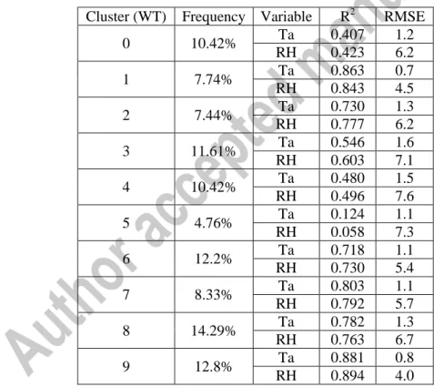
individual cluster varies. For Ta and RH, only Clusters 0, 4 and 5 show R2 lower than 0.5 while the rest of the clusters present much higher values, reaching in the case of Cluster 9, 0.881 and 0.894 for Ta and RH, respectively. In all the clusters, RMSE varies between 0.7 ⁰ C and 1.6 ⁰ C for Ta, and between 4.0% and 7.6% for RH (Table 5).
Table 5 Quantitative measures of clustered hourly air temperature (Ta) and relative humidity (RH) with respect to
available hourly data associated with each cluster (WT)
Cluster (WT) Frequency Variable R2 RMSE 0 10.42% Ta 0.407 1.2 RH 0.423 6.2 1 7.74% Ta 0.863 0.7 RH 0.843 4.5 2 7.44% Ta 0.730 1.3 RH 0.777 6.2 3 11.61% Ta 0.546 1.6 RH 0.603 7.1 4 10.42% Ta 0.480 1.5 RH 0.496 7.6 5 4.76% Ta 0.124 1.1 RH 0.058 7.3 6 12.2% Ta 0.718 1.1 RH 0.730 5.4 7 8.33% Ta 0.803 1.1 RH 0.792 5.7 8 14.29% Ta 0.782 1.3 RH 0.763 6.7 9 12.8% Ta 0.881 0.8 RH 0.894 4.0
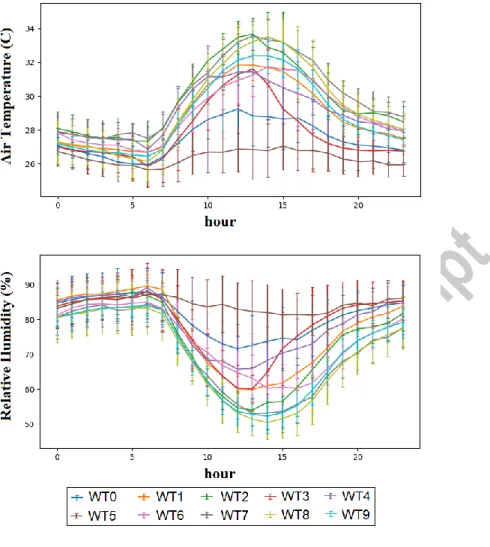
Fig. 4 shows the mean hourly evolution of Ta and RH for each of the WTs. Some of them (e.g. WT 4, 7, 8 and 9) have similar characteristics. However, as presented in section 2.2, other climatic variables (e.g. WS, WD and SolRad) make the difference between the WTs (Table 6).
Fig. 4 Hourly evolution of air temperature and relative humidity of the 10
weather types (WT) used as boundary conditions for ENVI-met.
Regarding WS, WD and Cloud Cover, the performance of each cluster is also different. In this case, since the model used for thermal comfort simulations (section 2.3.1) requires constant input values for these variables, the representativeness of each WT is based on daily mean values and standard deviation calculated from the hourly data included in each the clusters. Table 6, shows the results for all the clusters. WD values (daily mean) seem reasonable with a high percentage of situations with flow coming from the SW and NE which are the most prevailing WDs in Singapore (section 2.1). WS also agrees with the expected intensity of each typical WD in Singapore. However, the deviation of the daily mean WS in each cluster is relevant, and Cloud Cover mean values present little differences between WTs. In this sense, available data of Cloud Cover measured in Changi is not sufficiently precise for the evaluation of thermal comfort, an observation justified by different solar radiation values associated with a similar Cloud Cover value. This is the case of WT 2 and 4, which have the same daily mean Cloud Cover but different daily mean solar radiation (i.e. 467.5 and 342 Watt/m2 respectively). To avoid the use of misleading Cloud Cover data in the modelling of thermal comfort, a solar factor (feature of ENVI-met model) was used to correct the incoming solar radiation solved by the model with respect to the real value estimated in the clusters (see section 2.3.2).
Results are optimal in the sense that the 10 WTs agree with the climatic characteristics of our study area and can be associated with a meteorological condition occurring at a specific season (see section 3.3).
However, a more detailed analysis would have had to consider the inter-annual variability of climate. In this study we only used data from year 2016 to demonstrate the validity and necessity of the clustering approach to assess annual outdoor thermal comfort. Although a longer dataset (e.g. 5-10 years) could change the results and the quantitative measures of the clustered data, it is not expected a relevant difference due to the characteristics of climate in Singapore (see section 2.1).
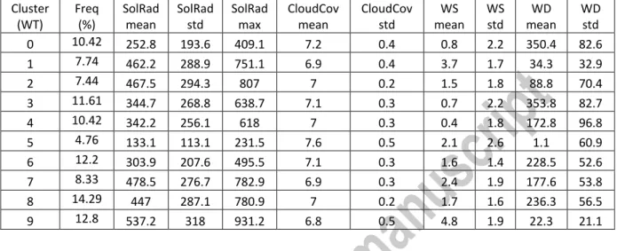
Table 6 Frequency of occurrence of each WT, and mean value and standard deviation of solar radiation
(Watt/m2), cloud cover (oktas), wind speed (m/s) and direction (º).
Cluster (WT) Freq (%) SolRad mean SolRad std SolRad max CloudCov mean CloudCov std WS mean WS std WD mean WD std 0 10.42 252.8 193.6 409.1 7.2 0.4 0.8 2.2 350.4 82.6 1 7.74 462.2 288.9 751.1 6.9 0.4 3.7 1.7 34.3 32.9 2 7.44 467.5 294.3 807 7 0.2 1.5 1.8 88.8 70.4 3 11.61 344.7 268.8 638.7 7.1 0.3 0.7 2.2 353.8 82.7 4 10.42 342.2 256.1 618 7 0.3 0.4 1.8 172.8 96.8 5 4.76 133.1 113.1 231.5 7.6 0.5 2.1 2.6 1.1 60.9 6 12.2 303.9 207.6 495.5 7.1 0.3 1.6 1.4 228.5 52.6 7 8.33 478.5 276.7 782.9 6.9 0.3 2.4 1.9 177.6 53.8 8 14.29 447 287.1 780.9 7 0.2 1.7 1.6 236.3 56.5 9 12.8 537.2 318 931.2 6.8 0.5 4.8 1.9 22.3 21.1
In our work, outputs of the clustering procedure were adapted to the requirements of the model used for outdoor thermal comfort assessment (ENVI-met). Other models might need other input climate data, but the same clustering method could still be valid. This approach is especially useful in models that are based on Computational Fluid Dynamics (CFD) which require high computational costs. Other models like SOLWEIG (Lindberg et al. 2008, 2016) and Rayman (Matzarakis et al. 2007), based on radiation fluxes, can have less computation requirements. They can support large input datasets (e.g. annual hourly data) to assess long-term thermal comfort levels. However, the weather clustering approach may still be used to analyse in depth the impact characteristics (e.g. spatial distribution of thermal comfort levels) of representative meteorological conditions.
3.3 Climatic classification of weather types
Following a description of the WTs is presented:
WP0 describes 10.4% of the days. It represents a situation with low Tmax (29.2 ºC) and diurnal amplitude of air temperature. Global Incoming Radiation values are low (daily maximum, 409.1 Watt/m2, and daily mean, 252.8 Watt/m2). Cloud cover is expected to be high and precipitation will occur (relative humidity is significantly high during daytime). WS is low and WD is variable but with a North component. This WT is not specific to a climate season of Singapore and thus can occur at any time along the year.
WT1 represents 7.7% of the days, with mid-range values of Tmax (31.9 ºC) and high maximum incoming solar radiation (751.1 Watt/m2). WS is high during daytime (5.1 m/s) but reduces significantly during night-time (1.9 m/s). WD is from the NE and quite constant. At midday, relative humidity is not high (60 %) and no or little precipitation can be expected. This day can be representative of the NE Monsoon
WT2 accounts for 7.4% of the days with highest Tmax (33.5 ºC) and highest maximum global radiation (807 Watt/m2). WD is variable with E component (NE in night-time and SE in daytime) and WS is low (1.5 m/s). Relative humidity is low (54%) at midday and no or little precipitation
is expected. This WT can occur in any season but is more likely in the Inter-monsoon and in the middle of the year.
WT3 describes 11.6% of the days. It represents a situation with mid-range values of Tmax (31.4 C). Incoming solar radiation presents mid values (daytime mean is 344.7 Watt/m2 and maximum is 638.7 Watt/m2). WD is variable with N component changing from NW to NE at midday. WS is low (0.7 m/s). Daytime relative humidity values are moderate (in the middle of the observed range) and increase during the afternoon. Precipitation is expected to occur, especially during the afternoon. These conditions can be representative of any period of the year with cloudy skies.
WT4 represents 10.4% of the days with mid-range Tmax (31.4 ºC). Temperature amplitude along the day is small (i.e. high daily minimum temperatures). Incoming solar radiation presents moderate values (similar to cluster 3). During night-time, WD is variable and WS is very low. However, during daytime WS increases at midday and afternoon to 1.7 m/s with prevailing WD from the S-SW. Daytime relative humidity values show moderate values and increase during the afternoon. Precipitation is expected to occur, especially during the afternoon. This WT is
characteristic of the Inter-monsoon season due to low WS and sea breeze development from SW.
WT5 accounts for 4.8% of the days and shows no relevant change in temperature values. These are low (Tmax: 26.9 ºC and Tmin: 25.6 ºC). Radiation is the lowest registered in Singapore (daytime mean is 133.1 Watt/m2 and maximum is 231.5 Watt/m2). Similarly, cloud cover is highest is Singapore. WD is quite constant during the day and close to the N. WS is similar during all day with mid values (2.1 m/s). Relative humidity is extremely high during all day (83%) and severe precipitation can be expected. These days are representative of the wet NE Monsoon with heavy rain all throughout the day, and low temperatures.
WT6 represents 12.2% of the days. It shows moderate Tmax (31.8 ºC). Incoming Solar Radiation are mid-low (daytime mean is 303.9 Watt/m2 and maximum is 495.5 Watt/m2). WD is constant from SW during all day with WS increasing during daytime to 2.8 m/s. Daytime relative humidity values show moderate values, and little and sparse precipitation can be expected. This WT is characteristic of the Inter-monsoon season with sea breeze development or the SW monsoon with some precipitation.
WT7 describes 8.3% of diurnal of climate conditions in Singapore. It presents highest Tmax (33.6 C) and also high maximum incoming solar radiation (782.9 Watt/m2). Cloud cover is low for Singapore. WD is constant with S component (SE during night-time and S during daytime) and mid WS values (2.4 m/s). Relative humidity is low (53%) at midday. These days are
representative of the SW Monsoon (in the middle of the year) with no precipitation.
WT8 accounts for 13.4% of the days. Its characteristics are quite similar to WT7, except that WD remains mostly constant from the SW and WS is slightly lower. These days are representative of the SW Monsoon (in the middle of the year) with no precipitation but also can be associated with sea breezes in the Inter-monsoon season (April, May).
WT9 represents 12.8% of the days with high Tmax (32.4 ºC) and the highest incoming solar radiation (931 Watt/m2). Cloud cover is lowest in Singapore. WD is constant and from NE during all day. WS is high during daytime (6 m/s) but reduces during night (2.5 m/s). Relative humidity at midday corresponds to the lowest (52.2%) in Singapore, and no precipitation is expected during these days. They are representative of the NE Monsoon in the dry period.
The information included in each of the previous WTs is considered suitable to analyze thermal comfort in our study area in Singapore. Although a climate dataset of several years could have been used (as discussed in section 3.2), the results presented agree with the climate characteristics of Singapore regarding prevailing wind flow and intensity and ranges of temperatures and relative humidity (see section 2.1). In this sense, the k-means statistical method is proved to be adequate to the construction of diurnal cycles of T and RH, and can also represent relatively well air flow on a daily basis.
The main advantage of applying this method to thermal comfort assessment is that it allows a complete assessment of the microscale thermal environment on an annual basis. Due to high demand of
computational resources, thermal comfort evaluation on a high spatial resolution has been frequently carried out using one or several meteorological conditions often extracted from one or several days of records in a meteorological station. Conclusions extracted from these evaluations can be misleading due to the use of data that does not represent the whole range of meteorological conditions to which an area is exposed.
The 10 WTs in our study describe meteorological conditions on a diurnal basis that manage to represent the conditions during the year. These 10 diurnal meteorological conditions can then be related to thermal comfort levels (spatially distributed) by the use of modelling techniques (see section 2.3). Since the percentage of occurrence of each WT is known, a better understanding of the temporal distribution of thermal comfort levels is available. Together with the spatial distribution of thermal comfort levels, information of the temporal variations is relevant to fine tune decision-making and urban design in the context of outdoor thermal comfort.
3.4 Impact of weather types on the thermal environment
3.4.1 Climate variables
In our study area, the distribution of values of T, RH, WS, Tmrt show relevant difference between the weighted mean values (including all the WTs) and the values of individual WTs.
Fig. 5 Distribution of climatic values (Wind Speed, Air Temperature, Mean Radiant Temperature and
Relative Humidity) in the courtyard area. Weighted mean values for all WTs as well as values for WT8 are presented.
Fig. 5 presents the distribution of T, RH, WS and Tmrt values at different hours for weighted mean values and for WT8. The comparison of both highlights the different distribution of climatic values. As expected WT8 has higher levels of T and Tmrt (already mentioned in section 3.3), especially during daytime.
Actually, WT8 is representative of a situation with high thermal stress (high solar radiation, high air temperature and low wind speed), which is a common meteorological condition used in many thermal comfort studies (Ali-Toudert and Mayer 2007; Ng et al. 2012; Yang et al. 2015, 2016). Thus, it turns that using a unique meteorological condition will lead to wrong conclusions if the overall thermal comfort levels of the study area are meant to be analyzed (see section 3.4.2).
Although results from some WTs differ less from the weighted mean results, none of them could represent thoroughly the ten WTs defined for our case study. Spatial median values of T, RH and WS at 9h, 12h, 15h, 18h, 21h of WT1 and WT6 show low difference with respect to the weighted mean results (Table 7). However, at midday and afternoon spatial median Tmrt values of WT3 and WT4 are closer to the weighted mean values that consider all the WTs.
The highest differences with respect to weighted mean values occur specially in WT5 for RH and Tmrt in accordance with the low solar radiation and high level of precipitation expected in these days (see section 3.3). On the contrary, WTs with higher solar radiation levels (e.g. WT9), show higher Tmrt values than mean weighted values, during midday and afternoon.
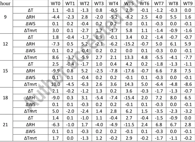
Table 7 Difference in spatial median values between the median weighted variables and the individual
WT results (in our study area). ∆T= Tw-Ti; ∆RH= RHw-RHi; ∆WS= WSw-WSi; ∆Tmrt= Tmrtw-Tmrti. (subindex w represent the weighted mean values and subindex i represents the individual WT value).
hour
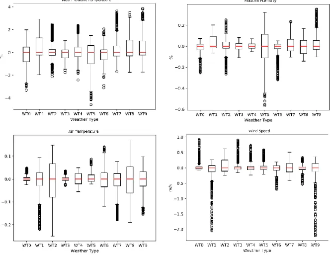
WT0 WT1 WT2 WT3 WT4 WT5 WT6 WT7 WT8 WT9 ∆T 1.1 -0.1 -1.3 0.8 -0.5 2.0 -0.1 -1.2 -0.3 0.0 9 ∆RH -4.4 -2.3 2.8 -2.0 -5.2 -8.2 2.5 4.0 5.5 1.6 ∆WS 0.1 0.2 -0.4 0.2 0.2 0.0 0.1 -0.3 0.0 -0.1 ∆Tmrt 3.0 0.1 -2.7 1.7 -1.7 5.8 1.1 -1.4 -0.9 -1.6 ∆T 1.8 -0.4 -1.7 0.9 -0.1 3.4 0.2 -1.4 -0.7 -0.7 12 ∆RH -7.3 0.5 5.2 -2.1 -6.2 -15.2 -0.7 5.0 6.1 5.9 ∆WS 0.1 0.2 -0.4 0.2 0.2 0.0 0.1 -0.3 0.0 -0.1 ∆Tmrt 8.6 -3.7 -5.9 2.7 2.1 13.3 4.8 -5.5 -4.1 -7.7 ∆T 2.5 -0.4 -1.7 1.0 0.4 4.2 0.2 -1.8 -1.3 -1.1 15 ∆RH -9.9 0.8 5.2 -2.5 -7.8 -17.6 -0.7 6.6 7.8 7.5 ∆WS 0.1 0.1 -0.4 0.2 0.2 -0.1 0.1 -0.3 0.0 -0.1 ∆Tmrt 10.0 -4.5 -6.3 2.6 3.6 14.3 5.0 -6.4 -4.8 -8.6 ∆T 2.1 -0.2 -1.2 1.3 0.2 3.6 -0.3 -1.7 -1.3 -0.7 18 ∆RH -9.0 0.3 3.1 -5.4 -7.4 -15.4 2.0 7.2 8.0 6.5 ∆WS 0.1 0.1 -0.3 0.2 0.2 -0.1 0.1 -0.3 0.0 -0.1 ∆Tmrt 5.0 -2.0 -2.4 1.4 2.8 6.2 1.5 -3.5 -2.3 -3.2 ∆T 1.4 0.1 -1.0 1.1 -0.4 2.7 -0.4 -1.5 -0.9 0.0 21 ∆RH -6.3 -1.0 1.7 -4.0 -4.9 -11.5 2.4 6.8 6.7 2.8 ∆WS 0.1 0.1 -0.3 0.2 0.2 -0.1 0.1 -0.3 0.0 -0.1 ∆Tmrt 1.7 0.0 -1.3 1.2 -0.2 2.9 -0.2 -1.7 -1.1 -0.2 Additionally, the spatial distribution of climatic values in the courtyard is different in each WT. Fig. 6 presents for hour 15:00 the range of differences between the weighted mean values and the individual WT values. In our study, WT5 shows a high spread of ∆Tmrt (Tmrtw-Tmrti; where subindex w represent the weighted mean values and the subindex i represents the individual WT value) followed by WT1, WT8 and WT9. It is important to notice that there is no relationship between the spatial median differences of∆T, ∆RH, ∆WS, ∆Tmrt (Table 7) and the range of values in the courtyard. This is the case of the WT2 and WT7, which show a different pattern of ∆Tmrt values (Fig. 6) while the spatial median difference is very similar. A similar situation occurs for ∆T, ∆RH and ∆Tmrt when we compared WT8 and WT9. Thus, with respect to the weighted mean values each individual WT presents a different spatial
distribution and range of climatic values depending of the interaction on the weather condition with the case study location. Higher spatial median differences between a WT and the weighted mean values are not associated with a higher spread of values in the courtyard.
These results are again relevant for urban planning since it is important to know accurately the spatial climatic differences in a study area to assure a better definition of uses of spaces in accordance with the local microclimate and thermal comfort.
Fig. 6 Normalized box plots of climate values difference between the weighted mean values (considering
all WTs) and each individual WT at 15.00 h. Each climate variable and WT has been normalized by the spatial median value.
3.4.2 Thermal comfort
As presented in the previous sections, different WTs affect in a different way climate variables inside the courtyard. The temporal evolution and spatial distribution of climatic values in each individual WTs differ from the weighted mean values (including all WTs) and thus affect levels of thermal comfort.
In our study area each WT produces a different impact on thermal comfort and thus a different percentage of area that meets a thermal comfort acceptability criteria.
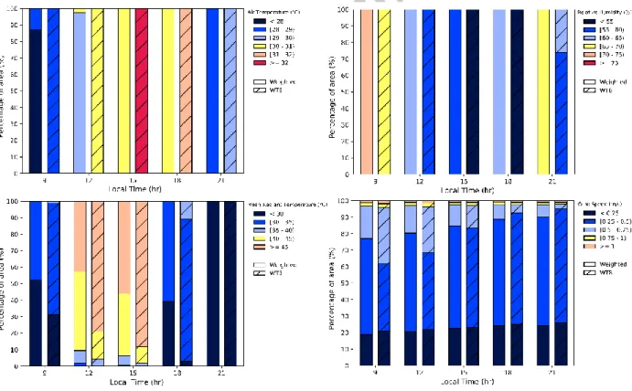
Considering the thermal comfort acceptability range defined for Singapore by Heng and Chow (2019), the whole courtyard (100% of the area) meets the acceptability criteria all the time (i.e. all the WTs) only at 21.00 h. At 12h and 15h no space inside the courtyard has acceptable thermal comfort levels throughout the year (Fig. 7). However, at these hours there are WTs when thermal comfort comes to be acceptable, at least in some parts of the courtyard. This is the case of WT0 that reaches the acceptability criteria in 40.6% and 46.7 % of the area at 12h and 15h, respectively. Even WT5 attains the criteria in the whole courtyard (100% of the area) at 12h and 15 h. (Fig. 8). Results correspond with the characteristics of the WTs affecting the study area (see section 3.3).
Fig. 7 Percentage of area in the courtyard that meets the thermal acceptability criteria all time (i.e. in all
WTs)
Comparison between the area with acceptable thermal comfort in one WT and the area that attains the acceptability criteria in all the WTs, shows significant differences in accordance with the climatic values and their spatial distribution for each WT. This is clear during the evening (18 h), when 5 WTs (WT0, WT3, WT4, WT5, WT6) attain a thermal acceptable situation in 100% of the area, representing 49.4% of the time throughout the year. However, at the same time of the day (18h) when considering all the WTs (i.e. 100% of the year), there is only 4.4% of the area that matches the acceptable thermal comfort range (Fig. 7).
Even if we consider a heat stress situation like WT8 when the percentage of courtyard that reaches an acceptable thermal comfort is low (0%, 0% and 24.4% at 12h, 15h and 18h, respectively), we find that including the rest of the WTs reduces more the percentage of area. Thus, if we consider all the weather types there will 19.9% less of area at 18h with acceptable thermal comfort than in WT8 (Fig. 8).
Fig. 8 Difference (in percentage) of area that meets the thermal comfort acceptability criteria between the
individual WTs and all WTs
These results justify a significant difference in the levels of thermal comfort both in the spatial and temporal scale when comparing unique weather condition versus a complete set of representative conditions. Misleading conclusions can outcome if outdoor thermal comfort is not evaluated in all
climatic situations. This is a relevant issue since urban design needs to consider all the weather conditions so as to provide a suitable and more convenient environment in larger spaces and during a higher number of hours. However, it should be considered that not all outdoor spaces require the same levels of thermal comfort and not all of them are used during all the time. Thus, it is relevant to use reliable and detailed information (spatial and temporal distribution) of the existing or predicted thermal comfort levels to define the use or purpose of different outdoor spaces.
4. Conclusions
This study presents a new approach for outdoor thermal comfort assessment. Contrary to previous studies when only certain weather conditions were evaluated (usually a high thermal stress situation), we now show the importance of analyzing all the relevant weather conditions which a specific urban area is exposed to.
The clustering method to obtain WTs from long term weather files has proved to be reliable and adequate for thermal comfort analysis in Singapore. In this case, 10 weather types have been defined to represent the main features of typical-day weather conditions in our study area. These seem reasonable regarding the small annual variation of climate conditions in Singapore and also can be considered suitable from a computational effort perspective. The quantitative measures of the clusters performance (i.e. how the weather types represent the available/measured data) show adequate values for a thermal comfort evaluation.
As expected, climate values vary significantly between WTs. Also spatial and temporal patterns are different in each WT. Results have shown that the percentage of surface attaining the thermal comfort acceptability criteria has relevant differences between weather conditions. Thus, inadequate and incomplete conclusions in a thermal comfort assessment can appear if all climatic situations are not evaluated.
The main advantage of applying this method is that it allows a complete assessment of the thermal environment on an annual basis by overcoming costly computational requirements of models that
evaluate wind dynamics (i.e. CFD) in the microscale. With the approach presented in this work the whole range of representative weather conditions are analyzed avoiding misleading evaluations on the thermal comfort levels of an area.
Although this study is focused on a courtyard the outcomes can be extended to other urban areas. Overall, it proposes a methodology to be implemented in the evaluation of thermal comfort and can help urban design by providing more accurate information that can improve the definition of use of outdoor spaces considering different weather conditions along the year. Similarly, the impact of mitigation measures would be more reliable and accurate considering all weather conditions.
Acknowledgements
The authors would like to thank XianXiang Li for his support and many other researchers in CENSAM-SMART, National University of Singapore (NUS), Singapore ETH Center (SEC) and Technical University of Munich (TUM)for the fruitful discussions in the framework of ‘Cooling Singapore’ project.
The work leading to these results was financially supported by the Singapore National Research
Foundation (NRF) under its Campus for Research Excellence And Technological Enterprise (CREATE) programme.
5. References
Acero JA, Arrizabalaga J (2018) Evaluating the performance of ENVI-met model in diurnal cycles for different meteorological conditions. Theor Appl Climatol 131:455–469. doi: 10.1007/s00704-016-1971-y
Acero JA, Herranz-Pascual K (2015) A comparison of thermal comfort conditions in four urban spaces by means of measurements and modelling techniques. Build Environ 93:245–257. doi:
10.1016/j.buildenv.2015.06.028
Ali-Toudert F, Mayer H (2006) Numerical study on the effects of aspect ratio and orientation of an urban street canyon on outdoor thermal comfort in hot and dry climate. Build Environ 41:94–108. doi: 10.1016/j.buildenv.2005.01.013
Ali-Toudert F, Mayer H (2007) Effects of asymmetry, galleries, overhanging façades and vegetation on thermal comfort in urban street canyons. Sol Energy 81:742–754. doi:
10.1016/j.solener.2006.10.007
Beck C, Philipp A (2010) Evaluation and comparison of circulation type classifications for the European domain. Phys Chem Earth, Parts A/B/C 35:374–387. doi: 10.1016/j.pce.2010.01.001
Besir AB, Cuce E (2018) Green roofs and facades: A comprehensive review. Renew Sustain Energy Rev 82:915–939. doi: 10.1016/j.rser.2017.09.106
Bruse M, Fleer H (1998) Simulating surface-plant-air interactions inside urban environments with a three dimensional numerical model. Environ Model Softw 13:373–384. doi:
10.1016/S1364-8152(98)00042-5
Chen L, Ng E (2012) Outdoor thermal comfort and outdoor activities: A review of research in the past decade. Cities 29:118–125. doi: 10.1016/j.cities.2011.08.006
Chow WTL, Pope RL, Martin CA, Brazel AJ (2011) Observing and modeling the nocturnal park cool island of an arid city: Horizontal and vertical impacts. Theor Appl Climatol 103:197–211. doi: 10.1007/s00704-010-0293-8
Chow WTL, Roth M (2006) Temporal dynamics of the urban heat island o Singapore. Int J Climatol 26:2243–2260. doi: 10.1002/joc
Demuzere M, van Lipzig NPM (2010) A new method to estimate air-quality levels using a synoptic-regression approach. Part I: Present-day O3and PM10analysis. Atmos Environ 44:1341–1355. doi: 10.1016/j.atmosenv.2009.06.029
Emmanuel R (ed) (2016) Urban Climate Challenges in the tropics. Rethinking Planning and Design Opportunities. Imperial College Press, London
Gulyás Á, Unger J, Matzarakis A (2006) Assessment of the microclimatic and human comfort conditions in a complex urban environment: Modelling and measurements. Build Environ 41:1713–1722. doi: 10.1016/j.buildenv.2005.07.001
Heng SL, Chow WTL (2019) How “hot” is too hot? Evaluating acceptable outdoor thermal comfort ranges in an equatorial urban park. Int J Biometeorol 63:801–816. doi: 10.1007/s00484-019-01694-1
Hidalgo J, Jougla R (2018) On the use of local weather types classification to improve climate understanding: An application on the urban climate of Toulouse. PLoS One 13:. doi: 10.1371/journal.pone.0208138
Hidalgo J, Masson V, Baehr C (2014) From daily climatic scenarios to hourly atmospheric forcing fields to force Soil-Vegetation-Atmosphere transfer models. Front Environ Sci 2:. doi:
10.3389/fenvs.2014.00040
Hoffmann P, Heinke SchlüNzen K (2013) Weather pattern classification to represent the urban heat island in present and future climate. J Appl Meteorol Climatol 52:2699–2714. doi: 10.1175/JAMC-D-12-065.1
Hong B, Lin B (2015) Numerical studies of the outdoor wind environment and thermal comfort at pedestrian level in housing blocks with different building layout patterns and trees arrangement. Renew Energy 73:18–27. doi: 10.1016/j.renene.2014.05.060
Höppe P (1999) The physiological equivalent temperature - a universal index for the biometeorological assessment of the thermal environment. Int J Biometeorol 43:71–75. doi: 10.1007/s004840050118
Huth R, Beck C, Philipp A, et al (2008) Classifications of atmospheric circulation patterns: Recent advances and applications. In: Annals of the New York Academy of Sciences. pp 105–152
Huttner S (2012) Further development and application of the 3D microclimate simulation ENVI-met. University of Mainz
Ignatius M, Wong NH, Jusuf SK (2015) Urban microclimate analysis with consideration of local ambient temperature, external heat gain, urban ventilation, and outdoor thermal comfort in the tropics. Sustain Cities Soc 19:121–135. doi: 10.1016/j.scs.2015.07.016
Jänicke B, Meier F, Hoelscher M-T, Scherer D (2015) Evaluating the Effects of Façade Greening on Human Bioclimate in a Complex Urban Environment. Adv Meteorol article ID:1–15. doi: http://dx.doi.org/10.1155/2015/747259
Ketterer C, Matzarakis A (2014) Human-biometeorological assessment of heat stress reduction by replanning measures in Stuttgart, Germany. Landsc Urban Plan 122:78–88. doi:
10.1016/j.landurbplan.2013.11.003
Krüger EL, Minella FO, Rasia F (2011) Impact of urban geometry on outdoor thermal comfort and air quality from field measurements in Curitiba, Brazil. Build Environ 46:621–634. doi:
10.1016/j.buildenv.2010.09.006
Li X-X, Norford LK (2016) Evaluation of cool roof and vegetations in mitigating urban heat island in a tropical city, Singapore. Urban Clim 16:59–74. doi: 10.1016/j.uclim.2015.12.002
Lindberg F, Holmer B, Thorsson S (2008) SOLWEIG 1.0 - Modelling spatial variations of 3D radiant fluxes and mean radiant temperature in complex urban settings. Int J Biometeorol 52:697–713. doi: 10.1007/s00484-008-0162-7
Lindberg F, Onomura S, Grimmond CSB (2016) Influence of ground surface characteristics on the mean radiant temperature in urban areas. Int J Biometeorol 60:1439–1452. doi: 10.1007/s00484-016-1135-x
Lobaccaro G, Acero JA (2015) Comparative analysis of green actions to improve outdoor thermal comfort inside typical urban street canyons. Urban Clim 14:251–267. doi:
10.1016/j.uclim.2015.10.002
Matzarakis A, Rutz F, Mayer H (2007) Modelling radiation fluxes in simple and complex environments--application of the RayMan model. Int J Biometeorol 51:323–34. doi: 10.1007/s00484-006-0061-8
Meteorological Service of Singapore (2017) Annual Climatological Report. Singapore
Meteorological Service Singapore (2016) The weather and climate of Singapore. Singapore
Morakinyo TE, Kong L, Lau KK-L, et al (2017) A study on the impact of shadow-cast and tree species on in-canyon and neighborhood’s thermal comfort. Build Environ 115:1–17. doi:
10.1016/j.buildenv.2017.01.005
Morris CJG, Simmonds I (2000) Associations between varying magnitudes of the urban heat island and the synoptic climatology in Melbourne, Australia. Int J Climatol 20:1931–1954. doi: 10.1002/1097-0088(200012)20:15<1931::AID-JOC578>3.0.CO;2-D
Müller N, Kuttler W, Barlag A-B (2014) Counteracting urban climate change: adaptation measures and their effect on thermal comfort. Theor Appl Climatol 115:243–257. doi: 10.1007/s00704-013-0890-4
Ng E (2009) Policies and technical guidelines for urban planning of high-density cities – air ventilation assessment (AVA) of Hong Kong. Build Environ 44:1478–1488. doi:
10.1016/j.buildenv.2008.06.013
Ng E, Chen L, Wang Y, Yuan C (2012) A study on the cooling effects of greening in a high-density city: An experience from Hong Kong. Build Environ 47:256–271. doi: 10.1016/j.buildenv.2011.07.014
Nishimura N, Nomura T, Iyota H, Kimoto S (1998) NOVEL WATER FACILITIES FOR CREATION OF COMFORTABLE URBAN MICROMETEOROLOGY. Sol Energy 64:197–207. doi: 10.1016/S0038-092X(98)00116-9
Oke TR (1987) Boundary Layer Climates. Routledge, New York
Pinto JG, Neuhaus CP, Leckebusch GC, et al (2010) Estimation of wind storm impacts over Western Germany under future climate conditions using a statistical-dynamical downscaling approach. Tellus, Ser A Dyn Meteorol Oceanogr 62:188–201. doi: 10.1111/j.1600-0870.2009.00424.x
Roth M, Chow WTL (2012) A historical review and assessment of urban heat island research in Singapore. Singap J Trop Geogr 33:381–397. doi: 10.1111/sjtg.12003
Roth M, Lim VH (2017) Evaluation of canopy-layer air and mean radiant temperature simulations by a microclimate model over a tropical residential neighbourhood. Build Environ 112:177–189. doi: 10.1016/j.buildenv.2016.11.026
Santamouris M, Synnefa A, Karlessi T (2011) Using advanced cool materials in the urban built
environment to mitigate heat islands and improve thermal comfort conditions. Sol. Energy 85:3085– 3102
Shashua-bar L, Erell E, Pearlmutter D (2009) WATER USE CONSIDERATIONS AND COOLING EFFECTS OF URBAN LANDSCAPE STRATEGIES IN A HOT DRY REGION. 2007–2010
Shen J, Chang SI, Lee ES, et al (2005) Determination of cluster number in clustering microarray data. Appl Math Comput 169:1172–1185. doi: 10.1016/j.amc.2004.10.076
Singapore Department of Statistics (2017) Population Trends 2016. Singapore
Steeneveld GJ, Koopmans S, Heusinkveld BG, Theeuwes NE (2014) Refreshing the role of open water surfaces on mitigating the maximum urban heat island effect. Landsc Urban Plan 121:92–96. doi: 10.1016/j.landurbplan.2013.09.001
Stewart ID, Oke TR (2012) Supplement DATASHEETS FOR LOCAL CLIMATE ZONES. Bull Am Meteorol Soc Meteor Soc 108–125. doi: 10.1175/BAMS-D-11-00019.2
Taleghani M, Berardi U (2016) The effect of pavement characteristics on pedestrians’ thermal comfort in Toronto. Urban Clim. doi: 10.1016/j.uclim.2017.05.007
Taleghani M, Kleerekoper L, Tenpierik M, van den Dobbelsteen A (2015) Outdoor thermal comfort within five different urban forms in the Netherlands. Build Environ 83:65–78. doi:
10.1016/j.buildenv.2014.03.014
Tan CL, Wong NH, Jusuf SK (2014) Effects of vertical greenery on mean radiant temperature in the tropical urban environment. Landsc Urban Plan 127:52–64. doi: 10.1016/j.landurbplan.2014.04.005
Weller HG, Tabor G, Jasak H, Fureby C (1998) A tensorial approach to computational continuum mechanics using object-oriented techniques. Comput Phys 12:620. doi: 10.1063/1.168744
Street in Singapore. J Urban Plan Dev 142:5015003. doi: 10.1061/(ASCE)UP.1943-5444.0000285
Yang W, Wong NH, Lin Y (2015) Thermal Comfort in High-rise Urban Environments in Singapore. Procedia Eng 121:2125–2131. doi: 10.1016/j.proeng.2015.09.083
Yang W, Wong NH, Zhang G (2013) A comparative analysis of human thermal conditions in outdoor urban spaces in the summer season in Singapore and Changsha, China. Int J Biometeorol 57:895– 907. doi: 10.1007/s00484-012-0616-9
Zölch T, Maderspacher J, Wamsler C, Pauleit S (2016) Using green infrastructure for urban climate-proofing: An evaluation of heat mitigation measures at the micro-scale. Urban For Urban Green 20:305–316. doi: 10.1016/j.ufug.2016.09.011