HAL Id: hal-01956023
https://hal.inria.fr/hal-01956023v2
Submitted on 6 Feb 2020
HAL is a multi-disciplinary open access
archive for the deposit and dissemination of sci-entific research documents, whether they are pub-lished or not. The documents may come from teaching and research institutions in France or abroad, or from public or private research centers.
L’archive ouverte pluridisciplinaire HAL, est destinée au dépôt et à la diffusion de documents scientifiques de niveau recherche, publiés ou non, émanant des établissements d’enseignement et de recherche français ou étrangers, des laboratoires publics ou privés.
cell model for growing and regenerating tissues
Paul Liedekerke, Johannes Neitsch, Tim Johann, Enrico Warmt, Ismael
Gonzàlez-Valverde, Stefan Hoehme, Steffen Grosser, Josef Kaes, Dirk Drasdo
To cite this version:
Paul Liedekerke, Johannes Neitsch, Tim Johann, Enrico Warmt, Ismael Gonzàlez-Valverde, et al.. A quantitative high-resolution computational mechanics cell model for growing and regenerating tissues. Biomechanics and Modeling in Mechanobiology, Springer Verlag, 2019, �10.1007/s10237-019-01204-7�. �hal-01956023v2�
https://doi.org/10.1007/s10237-019-01204-7
ORIGINAL PAPER
A quantitative high‑resolution computational mechanics cell model
for growing and regenerating tissues
Paul Van Liedekerke1,2 · Johannes Neitsch3 · Tim Johann2 · Enrico Warmt5 · Ismael Gonzàlez‑Valverde6 ·
Stefan Hoehme3,4 · Steffen Grosser5 · Josef Kaes5 · Dirk Drasdo1,2,3
Received: 21 November 2018 / Accepted: 16 July 2019 © Springer-Verlag GmbH Germany, part of Springer Nature 2019
Abstract
Mathematical models are increasingly designed to guide experiments in biology, biotechnology, as well as to assist in medi-cal decision making. They are in particular important to understand emergent collective cell behavior. For this purpose, the models, despite still abstractions of reality, need to be quantitative in all aspects relevant for the question of interest. This paper considers as showcase example the regeneration of liver after drug-induced depletion of hepatocytes, in which the surviving and dividing hepatocytes must squeeze in between the blood vessels of a network to refill the emerged lesions. Here, the cells’ response to mechanical stress might significantly impact the regeneration process. We present a 3D high-resolution cell-based model integrating information from measurements in order to obtain a refined and quantitative understanding of the impact of cell-biomechanical effects on the closure of drug-induced lesions in liver. Our model represents each cell individually and is constructed by a discrete, physically scalable network of viscoelastic elements, capable of mimicking realistic cell deformation and supplying information at subcellular scales. The cells have the capability to migrate, grow, and divide, and the nature and parameters of their mechanical elements can be inferred from comparisons with optical stretcher experiments. Due to triangulation of the cell surface, interactions of cells with arbitrarily shaped (triangulated) structures such as blood vessels can be captured naturally. Comparing our simulations with those of so-called center-based models, in which cells have a largely rigid shape and forces are exerted between cell centers, we find that the migration forces a cell needs to exert on its environment to close a tissue lesion, is much smaller than predicted by center-based models. To stress generality of the approach, the liver simulations were complemented by monolayer and multicellular spheroid growth simulations. In summary, our model can give quantitative insight in many tissue organization processes, permits hypothesis testing in silico, and guide experiments in situations in which cell mechanics is considered important.
Keywords Cell-based model · High resolution cell model · Cell mechanics · Liver regeneration · Optical stretcher
Electronic supplementary material The online version of this article (https ://doi.org/10.1007/s1023 7-019-01204 -7) contains supplementary material, which is available to authorized users. * Paul Van Liedekerke
[email protected] * Dirk Drasdo
1 Inria Paris & Sorbonne Université LJLL, 2 Rue Simone IFF,
75012 Paris, France
2 IfADo - Leibniz Research Centre for Working Environment
and Human Factors, Ardeystrasse 67, Dortmund, Germany
3 Interdisciplinary Centre for Bioinformatics, Leipzig
University, Härtelstr. 16–18, 04107 Leipzig, Germany
4 Institute for Computer Science, Leipzig University,
Härtelstr. 16–18, 04107 Leipzig, Germany
5 Faculty of Physics and Earth Science, Peter Debye Institute
for Soft Matter Physics, Leipzig University, Linnéstraße 5, 04103 Leipzig, Germany
6 M2be, University of Zaragoza, C/ Maria de Luna s/n,
1 Introduction
Driven by the insight that multicellular organization cannot be explained from the viewpoint of biochemical processes alone and flanked by recent development of methods in imag-ing and probimag-ing of physical forces at small scales, the role of mechanics in the interplay of cell and multicellular dynamics is moving into the main focus of biological research (Fletcher
and Mullins 2010). Cells respond on mechanical stress both
passively and actively; hence, an understanding of the growth and division behavior of proliferating cells is not possible without properly taking into account the mechanical compo-nents underlying these processes. Mathematical models are being established as an additional cornerstone to interpret biological observations and provide information to clinicians
entering in their decisions (Rodriguez et al. 2013; Karolak
et al. 2018). This requires high reliability of models and
quantitative simulations.
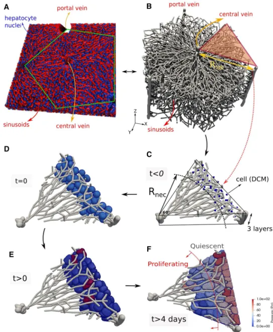
A clinical relevant example is the regeneration of liver after drug-induced toxic damage after paracetamol (acetami-nophen, APAP) or tetrachloride (CCl4) overdose. These drugs generate a characteristic central necrotic hepatocyte-depleted lesion in each liver lobule, which is the smallest repetitive
functional and anatomical unit of liver. Hoehme et al. (2010)
used confocal laser scanning micrographs to set up a real-istic spatial-temporal agent-based model of a liver lobule. In their model, hepatocytes were represented as individual units (agents) parameterized by biophysical and biological quantities and able to move as a consequence of forces on the cell, and of the cells’ own micro-motility. The cells were approximated as spheres (the shape a cell adopts in isola-tion), while the forces between them are simulated as forces between the cell centers, which is why these models are often termed “center-based model” (CBM). Center-based models have proven useful to mimic tissue organization processes, for example, in vitro and in early development (see, e.g., Drasdo
and Höhme 2005; Drasdo et al. 2007; Geris et al. 2010; Buske
et al. 2011) and have been shown to provide a good framework
for multiscale simulations in tumor development (e.g.,
Ramis-Conde et al. 2009; Delile et al. 2017). For liver, the CBM
predicted that active uniform micro-motility forces would not suffice to close the characteristic necrotic tissue lesions gener-ated in the center of each liver lobule but further mechanisms as directed migration and oriented cell division along closest micro-vessels (named hepatocyte-sinusoid alignment, HSA) would be necessary to explain the observed regeneration sce-narios. HSA has been subsequently be experimentally vali-dated. To obtain these results, extensive simulated sensitivity analyses had been performed varying each parameter of the
model within its physiological range (Drasdo et al. 2014). In
order to arrive at such conclusions, the model must for a given set of parameters be able to realistically and quantitatively
predict the outcome of the regeneration process. The model can then be viewed as a mapping from a set of parameters to a set of macroscopic observables such as the size of the necrotic lesion or the cell density in the lobule.
A major drawback of center-based models is that they are based on the calculation of pairwise forces (usually Hertz force, Johnson–Kendall–Roberts force or related) between cell centers, which lack accuracy in dense cell aggregates under compression where the interaction force of a cell with one neighbor impacts on its interaction force with another neighbor. A consequence of a naive use of pairwise forces is the absence of a notion of cell volume. Hence, simulations with quasi-incompressible cells characterized by a Poisson ratio of 𝜈 ≈ 0.5 can lead to unrealistic multicellular arrange-ments and thus to false predictions. Such situation may occur during liver regeneration after APAP or CCl4 intoxication where many cells enter the cell cycle almost at the same time close the drug-induced lesion. It also occurs in the interior of growing multicellular spheroids. Model corrections have been proposed to circumvent this shortcoming, but so far a fully consistent approach for center-based models has been out of reach as this requires to consistently relate cell–cell interaction forces and cell shape. In center-based models, cell shape can only be estimated for very small cell defor-mations. Approximating cell shape by Voronoi-tessellation
Schaller and Meyer-Hermann (2005) permits to calculate a
cell volume, but the interaction forces are in most situations inconsistent with the cell–cell contact areas resulting from
this tessellation (Van Liedekerke et al. 2015).
The shortcomings of the CBM call for a model type that consistently relates cell strain and stresses in cells within multicellular assemblies. A large category of models called lattice-free, force-based “deformable cell models” (DCMs)
has been developed to meet these needs (Rejniak 2007;
Sandersius and Newman 2008; Jamali et al. 2010; Odenthal
et al. 2013; Van Liedekerke et al. 2019). Their lattice-based
counterparts, called cellular Potts models (CPM), are popular in biomedical modeling, partially because of their straight-forward implementation. The dynamics in CPM is princi-pally stochastic in nature and is based on the minimization of energy functionals (Hamiltonian) and Monte Carlo sampling over a vast number of lattice sites (e.g., Graner and Glazier
1992; van Oers et al. 2014; Palm and Merks 2013).
Force-based methods use equations of motion, which facilitates pre-senting both stochastic and deterministic components. Early work in this field has treated multicellular spheroids, vari-ous cellular patterns in developing ductal carcinoma in situ, invasive tumors as well as normal development of epithelial ductal monolayers and their various mutants (e.g., Galle et al.
2005, Rejniak 2007; Drasdo et al. 2007; Dillon et al. 2008;
Rejniak and Anderson 2008; Sandersius and Newman 2008).
Deformable models have also been developed to study the dynamics of erythrocytes in blood flow (Hosseini and Feng
2009; Fedosov et al. 2010; Van Liedekerke et al. 2013;
Fed-osov et al. 2011), cellular rheology (Sandersius et al. 2011),
or even impact of tissue (Van Liedekerke et al. 2010, 2011).
Recent approaches focus more and more on the explicit representation of subcellular details such as a nucleus, and
cytoskeleton (Jamali et al. 2010; Chen et al. 2018). Other
DCM types, such as the vertex model, focus intrinsically
more on epithelial sheets (Fletcher et al. 2014).
In this paper, we present an agent-based, high-resolution deformable cell model in three dimensions allowing to simu-late cell growth and tissues. The model is particularly suited to study the interplay between cell growth, mechanical vari-ables and tissue architecture and is here employed to mimic tissue regeneration in a part of a liver lobule. Our cell model
builds upon earlier work by Odenthal et al. (2013) and Van
Liedekerke et al. (2019), a DCM type whereby the cell surface
is triangulated and the nodes are connected by viscoelastic elements, representing the cell membrane and actin cortical cytoskeleton and homogeneous cytoplasm. In the work of Odenthal et al., it was shown that this DCM could quanti-tatively mimic the adhesion dynamics of red blood cells on a surface, yet cell growth and division were not envisaged. Here, we enrich the model with those features, enabling us to model various multicellular systems. DCM types with cell division capabilities have been created by a number of authors (e.g., Jamali et al. 2010; Tanaka et al. 2015; Milde et al. 2014),
whereby in Jamali et al. (2010) the mechanical processes
lead-ing to cytokinesis have been explicitly mimicked. Most of these models are two-dimensional. Cytokinesis, during which a cell splits into two separated daughter cells, completes the mitosis phase. Mitosis and cytokinesis together take about 1 h compared to the duration of the cell cycle ∼ 24 h in most mammalian cells, hence are very short. Accurate simulation of the cytokinesis process in three-dimensional triangulated cells turns out to be challenging with regard to both the algorithms
and computational efforts. For these reasons, our DCM1
mim-ics the cell division event in one step, yet ensuring that the daughter cells precisely fill the space of the mother cell.
Our model has basically two key advantages. First, the model can be parameterized by physical and biokinetic parameters. By direct comparison with optical stretcher
exper-iments (Guck et al. 2001), which cause cell deformation as a
response of an externally applied stress by a laser beam, we determine the type of the cell’s viscoelastic elements and the magnitude of its parameters. In addition to the basic cortical triangulated model, we have created the possibility for each cell to mimic an internal cytoskeleton by connecting the cell cortex and the cell nucleus by viscoelastic elements. However, as we have found that the deformation of cells can quantita-tively be captured even without explicit representation of cell
nuclei, we perform the simulations in this paper discerning only the cell boundary elements. Second, the model design is such that each cell can interact with any arbitrarily shaped objects that are either represented by a triangulated surface (rigid of flexible, see, for example, Fig. 11), which can also be generated by external specialized software, or represented by a mathematical surface. The model is not restricted to simu-late elementary structures such as spheroids or monolayers. In liver architecture, relevant for our final application example, cells interact with other cells, but also with a complex network of micro-vessels (named liver sinusoids).
The approach facilitates performing hybrid tissue simula-tions where DCM cells can interact with center-based cells. Generally, hybrid simulations are useful if simulations of an entire tissue need to be performed in a reasonable time
(González-Valverde and García-Aznar 2018). Hybrid modeling
combining DCM and center-based model, conceptually similar
to the hybrid strategy proposed in Kim et al. (2013), enables us
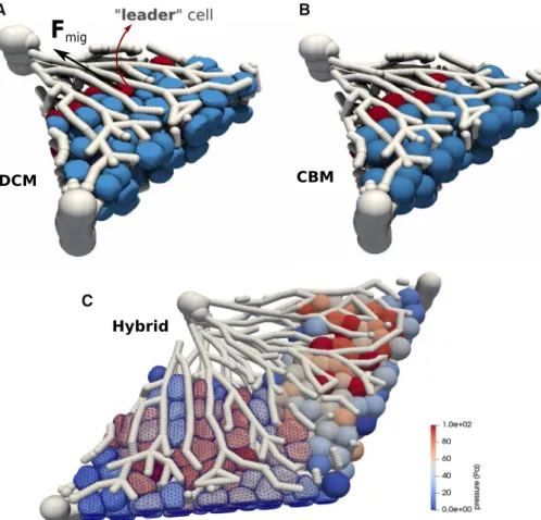
to simulated part of the system as higher spatial resolution and thereby “zoom” into spatial substructures of interest. To ensure that the center-based model behaves “on average” as the DCM, which is a priori not the case due to the shortcomings of the CBM approach as discussed above, we here propose a simple correction scheme in which the interaction forces of the CBM are calibrated from simulations with the DCM. In this way, the DCM can be used to verify the systems behavior of the CBM for small cell populations, while the CBM can be used to simulate large cell populations. We demonstrate this by direct comparison of a CBM and a DCM in the same liver lobule.
This paper is structured as follows. The technical details of the DCM and the CBM (and force calibration) are explained
in Sect. 2. Following, we first study the single cell
dynam-ics of the DCM. Each model parameter, biomechanical and biokinetic, can be directly associated with a physical prop-erty, i.e., can either be directly measured or be calibrated by comparison to single cell or multicellular experiments. This makes it possible to identify physiological parameter ranges. We here compare directly optical stretcher real to in silico
(with the DCM) experiments (Sect. 3.1.1) to identify the
nature of viscoelastic elements in the DCM and their param-eters. Next, we consider classical in silico experiments of two adhering cells being mechanically separated to identify the model parameters for cell–cell adhesion. We verify whether the contact forces and stress distribution on the cell surface
predicted by our model are physically plausible (Sect. 3.1.2).
These experiments can generally serve as means to calibrate the parameters of a single cell accurately. Secondly, we con-sider the growth and proliferation of the cells in the classical settings of growing monolayer and multicellular spheroids, which have been studied in numerous experiments and
mod-eling works (Sect. 3.2). Finally, we perform simulations of
regeneration dynamics after intoxication of liver with CCl4/ APAP using the DCM and compare simulation results to
1 From now on, we will use the term “DCM” uniquely for our
both experimental data and simulation results with the CBM
similar as in Hoehme et al. (2010). We analyze the results
and basic differences in terms of dynamics and tissue
archi-tecture in Sect. 3.3. The cell shapes obtained by simulations
with the DCM can in principle readily be compared with high-resolution confocal microscopy images (e.g.,
Morales-Navarrete et al. 2019). Together with developments in tissue
clearing (Tainaka et al. 2016) this might open up the
pos-sibility to infer the stresses on the cells in full 3D volume reconstructions from laser scanning confocal micrographs of the cell shapes. Alternatively, the elastic properties of emer-gent tissues simulated with the model can be compared to
elastographic images (Sack et al. 2013).
2 Mathematical models
In this section, we define the specific agent-based mathe-matical models that we use later in specific applications. In agent-based models of multicellular assemblies, every cell ( = agent) is represented as an individual separated object that is able to move, grow, divide, and die. The cell can interact with other cells as well as other objects in its environment. As such, emerging effects of these many interactions can be studied. We explain the two types of single cell-based models used in this work: first the deformable cell model (DCM), and then we recapitulate the center-based model (CBM).
2.1 Deformable cell model (DCM)
In our DCM, the cell surface is triangulated with viscoe-lastic elements along each edge of each triangle. This cre-ates a global deformable structure with many degrees of
freedom (Van Liedekerke et al. 2010; Odenthal et al. 2013;
Van Liedekerke et al. 2019; Guyot et al. 2016). Throughout
this paper, we do not represent the cell organelles sepa-rately, but by a homogeneous isotropic viscoelastic material
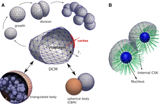
(see Fig. 1a). Nevertheless, our model in principle permits
the explicit representation of organelles, e.g., by triangulat-ing them in the same way as the cell surface and connecttriangulat-ing
the structures by viscoelastic elements (Fig. 1b).
We found that the homogenized approximation suf-ficed as the explicit representation of cell organelles was both not needed and computationally costly for the ques-tions studied in this paper. The viscoelastic elements and parameters of the cell surface are calibrated such that they simultaneously account for the mechanical response of the cell membrane and cell cortex, in particular the cortical cytoskeleton (CSK), i.e., forces that represent in-plane and bending elasticity of the cortex and the plasma membrane. Moreover, we account for a force combining contributions from the cytoplasm and the nucleus in response to cell compression. Cell–cell interactions induce external forces, which may be repulsive or adhesive, or both.
Cells in our model can migrate, die, grow, and divide when their volume has doubled. When a cell divides, two
Fig. 1 a The force-based deformable cell model (DCM) and its basic
components and functionality used in this work. A cell is represented by a viscoelastic triangulated shell (cortex) containing a compressible cyto-plasm (center). The cells can grow until they split into two new cells, eventually creating a clump of adhering cells (top). Each nodal point
of the cell moves according to an equation of motion in response to a force 𝐅i . The cells can interact with rigid triangulated bodies (such as here a capsule encapsulating them) or simple geometric bodies such as a center-based model (bottom). b Same model showing prototype of the model where a nucleus and internal cytoskeleton is included explicitly
new cells are created that fit in the envelope of the mother cell and all aforementioned forces are automatically
invoked on the daughter cells (see Fig. 3). Apoptosis can
be modeled as well. The details of the model components are explained in the following sections.
2.1.1 Forces and equations of motion
Movement and deformation of a cell can be calculated from a force balance summarized in the following equation of motion for each node i of the triangulation:
The terms denote (1) node–node friction of nodes belong-ing to the same cell, to mimic dampbelong-ing by the CSK of two nodes move relatively to each other; (2) node–node fric-tion of nodes belonging to different cells (alternatively, the first two terms as they have the same form could be casted into one term keeping in mind that the friction coefficients among nodes of the same cell and of a cell with another cell may differ); (3) friction between nodes of the cell and extracellular matrix (ECM) or liquid; (4) nodal forces due to CSK in-plane elasticity; (5) nodal forces due to CSK bending elasticity; (6) nodal volume force terms penalizing deviations from the cells’ intrinsic volume; (7) nodal forces due to membrane area conservation; (8) nodal contact forces consisting of a repulsive and adhesive part due to interac-tions with a substrate or other cells; and (9) nodal active migration forces.
Inertia terms have been neglected as the Reynolds num-bers of the medium circumventing the cells are very small
(Odell et al. 1981); this approximation is common for cell
movement (see, e.g., Van Liedekerke et al. 2015; Drasdo
et al. 2007). More specifically, the matrices 𝚪nn and 𝚪ns
rep-resent node–node friction and node substrate (ECM) friction, respectively. 𝐯i denotes the velocity of node i. The first term and the second term on the rhs. represent the CSK in-plane nodal elastic forces 𝐅e,ij and the bending force 𝐅m,i . The third
term on the rhs. is a volume force 𝐅vol,i and controls the cell
compressibility. We assume that cells are compressible on longer timescales controlled by in- and outflow of water. As water transport volume flow rates are small, on short time-scales cell volume can be only slightly compressed by com-pression of the elastic structures inside the cell such as the cytoskeleton; hence, the cell exhibits a near incompressible behavior. On longer timescales, the cell response may become more complex due to intracellular adaptations (Monnier et al. (1) ∑ j 𝚪cnn,ij(𝐯i− 𝐯j) ⏟⏞⏞⏞⏞⏞⏞⏞⏞⏟⏞⏞⏞⏞⏞⏞⏞⏞⏟ (1) +∑ k 𝚪ccnn,ik(𝐯i− 𝐯k) ⏟⏞⏞⏞⏞⏞⏞⏞⏞⏞⏟⏞⏞⏞⏞⏞⏞⏞⏞⏞⏟ (2) + 𝚪ns,i𝐯i ⏟⏟⏟ (3) =∑ j 𝐅e,ij ⏟⏟⏟ (4) +∑ m 𝐅m,i ⏟⏟⏟ (5) + 𝐅vol,i ⏟⏟⏟ (6) +∑ T 𝐅T,i ⏟⏟⏟ (7) + 𝐅rep,i+ 𝐅adh,i ⏟⏞⏞⏞⏞⏟⏞⏞⏞⏞⏟ (8) + 𝐅mig,i ⏟⏟⏟ (9) .
2016). The force 𝐅T,i accounts for resistance against isotropic
expansion of the cell membrane. The two terms ( 𝐅adh,i , 𝐅rep,i )
account for potential adhesion and repulsion forces on a local surface node, exerted by an external object such as other trian-gulated cells or rigid structures (see Fig. 1a). 𝐅mig,i describes
the migration forces acting on each node to result in a global movement of the cell. We now give more detail on how these forces and friction components can be calculated.
Friction terms (1–3): The matrices 𝚪c nn , 𝚪
cc
nn and 𝚪ns in Eq. 1
represent node–node friction and node substrate friction ten-sors, respectively. Friction between two nodes of the same cell mimics damping in the cortical CSK. Nodal friction terms with the cytosol are not explicitly accounted for but are partially incorporated in the node–node friction terms. Node-node fric-tion from different cells the mimics the fricfric-tion when their membranes slide along each other. Individual friction coef-ficients for two nodes are denoted as 𝛾k where k can refers to the nature of the contact (i.e., nodes on the same cell; nodes of two different cells; friction of a node with extracellular matrix; friction of a node with a liquid). Furthermore, we distinguish between friction in parallel ( 𝛾|| ) and normal ( 𝛾⟂ ) direction to
the relative motion. If the parallel and normal coefficients are not equal (anisotropy), the friction tensor becomes
with 𝐞ij= (𝐫j− 𝐫i)∕||𝐫j− 𝐫i|| , where ri , rj denote the position of the nodes of a cell. I is the 3 × 3 identity matrix, while ⊗ denotes the dyadic product. The nodal cell–substrate
fric-tion 𝛤ns can represent viscous resistance with liquid, ECM,
capillaries or membranes. If the cell is spherical and the
medium is isotropic, then 𝛤ns is a diagonal matrix.2 It can
be reasonable to split the friction coefficients—which have unit Ns/m—into a product of a friction coefficient per
sur-face area (unit Ns∕m3 ) and the shared surface area
associ-ated with the interaction of the two nodes (unit m2 ). The
nodal areas are calculated in the contact model (See Contact force model). In case of friction of a node i with an exter-nal medium, this surface area is the Voronoi region area of that node (from the dual graph of the surface triangulation), which is determined by the neighboring nodes (see Van
Liedekerke et al. 2017).
Cytoskeleton in-plane elasticity—term (4) in Eq. 1: The
CSK in-plane elasticity is controlled by the viscoelastic ele-ments. The elastic forces in the network of a cell cortex are in this model mimicked by linear springs with spring
stiff-ness ks . In combination with the node–node friction
coeffi-cients 𝛾int which endow the terms (1) of Eq. 1, the elements
become viscoelastic. Complex viscoelastic elements can be constructed by combining several springs and dashpots or using nonlinear springs.
(2) 𝚪nn,ij= 𝛾⟂(𝐞ij⊗𝐞ij) + 𝛾||(I − 𝐞ij⊗𝐞ij),
2 In this paper, we assume that friction with ECM is isotropic and
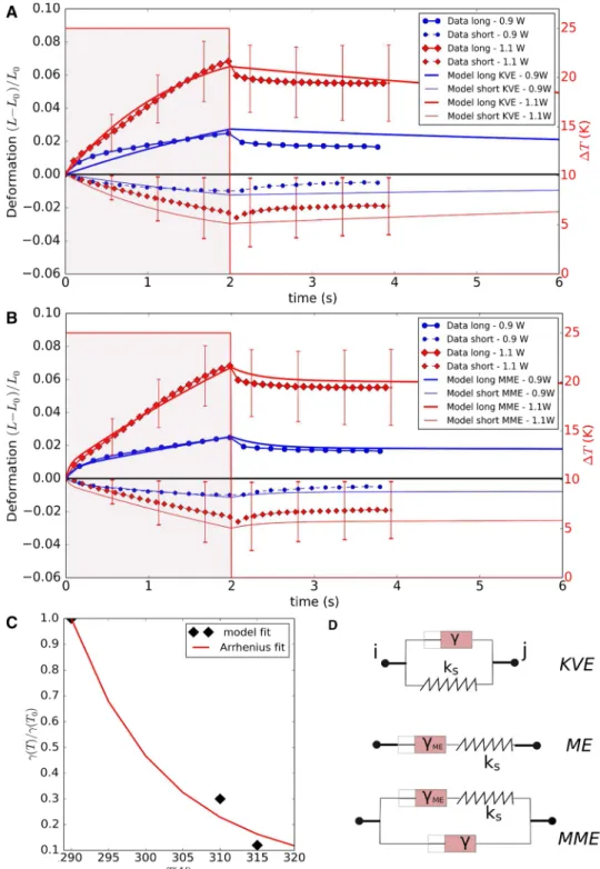
Let us first focus on a nodal subsystem in Eq. 1 in which the spring and friction terms are schematically positioned in parallel, representing a solid like behavior so that the ele-ments after release of an external force relax back to its orig-inal length. This is called the Kevin–Voigt Element (KVE)
(Fig. 5d). Consider the internal force Fint originating from
the Kelvin–Voigt viscoelastic element between node nodes i and j (for simplicity 𝛾||= 𝛾⟂= 𝛾).
where l0 ij=||𝐫 0 ij|| = ||𝐫 0 j − 𝐫 0
i|| and lij=||𝐫ij|| are the initial (cell at rest) and actual lengths between the nodes, and
𝐯ij= 𝐯i− 𝐯j is their relative velocity. The force balance
equa-tion with external forces 𝐅ext (external forces can be for
instance adhesion forces between nodes, see further)
demands that 𝐅ext+ 𝐅int= 𝟎 , hence:
Contrary, a Maxwell element (ME) simulates a fluid-like extension of the cortex. In the ME, the friction element and spring element are schematically positioned in series (see
Fig. 5d), which is why an external force leading to an
exten-sion of the element is damped but removal of the force does not lead to relaxation of the element back to its original length characteristic for a fluid behavior. The equation of
the internal force in the element 𝐅int (assuming isotropic
constants) reads
This equation contains a derivative of the force, which can be approximated by ̇𝐅int= (𝐅int(t) − 𝐅int(t − Δt))∕Δt . From
the force balance between external and internal forces, we find now:
This equation thus involves the evaluation of the internal
force on the previous time step.3
The linear spring constant ks for a sixfold symmetric tri-angulated lattice can be related approximately to the cortex
Young modulus Ecor with thickness hcor by Boal (2012)
(3) 𝐅int,ij = 𝐅e,ij− 𝛾𝐯ij
= − ks(lij− l0ij)𝐞ji− 𝛾𝐯ij,
(4) 𝐅ext,ij− ks(lij− l0ij)𝐞ji− 𝛾𝐯ij= 𝟎.
(5) ̇𝐅int,ij ks + 𝐅int,ij 𝛾ME = 𝐯ij. (6) 𝐅ext,ij(t) + 𝐅int,ij(t − Δt) 1+ ksΔt∕𝛾ME + kΔt 1+ ksΔt∕𝛾ME 𝐯ij= 𝟎.
Furthermore, the total elastic in-plane CSK forces can be related to a local in-plane stress using the virial formula:
where Ni is the coordination number of node i, Fint,ij is the
total elastic force between i and j.
We here do not assume an active contractile state of the cell. Cell contractility could be included in the model as an extra active elastic force term by, e.g., changing the element rest length l0 (see Odell et al. 1981), but this is not considered in this paper.
CSK bending force—term (5) in Eq. 1: The bending
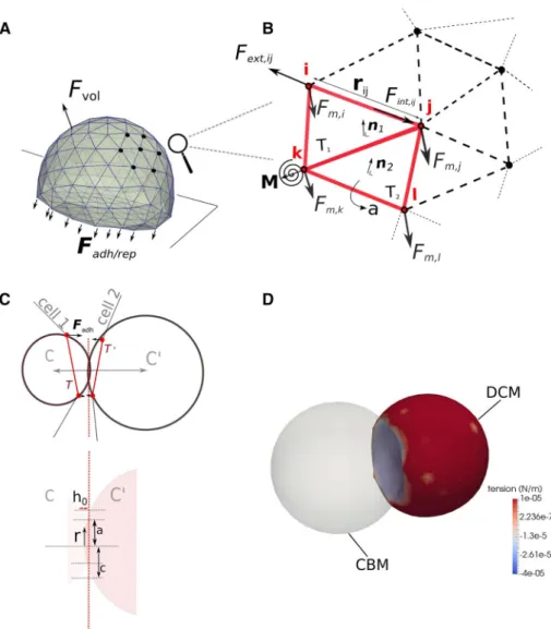
ance from the cortex is incorporated by the rotational resist-ance of the hinges determined by two adjacent triangles T1= {ijk} and T2= {ijl} (see Fig. 2b). This permits to define the bending moment M:
where kb is the bending constant specified below and 𝜃 is
the angle between the normal vectors to the triangles 𝐧1, 𝐧2
, determined by their scalar product (𝐧1𝐧2) = cos(𝜃) . 𝜃0 is
the angle of spontaneous curvature. The moment M can be
transformed to an equivalent force system 𝐅m,z ( z ∈ {ijkl} )
for the triangles T1 and T2 where for T1 we can compute
𝐅m,i= M∕l1𝐧1 using l1 as the distance between the hinge
of the triangle pair and the point i, and similar
expres-sion for 𝐅m,l . The forces working on nodes j, k must fulfill
𝐅m,i+ 𝐅m,j+ 𝐅m,k+ 𝐅m,l= 0 to conserve momentum. The
bending stiffness of the cortex is approximated by
where 𝜈 is the Poisson’s ratio of the cortex.
Volume force—term (6) in Eq. 1:
The nodal contact forces with the cytosol are in the standard model accounted for by the volume forces. These regulate the volume changes according to the applied pressure and the bulk
modulus property KV of the cell. The compressibility of the cell
depends on volume fraction of water in the cytosol, the CSK vol-ume fraction and structure, and the compressibility of the orga-nelles. In addition, it may be influenced by the permeability of the plasma membrane for water, the presence of caveolae (Sinha et al.
2011), and active responses in the cell. We calculate the internal pressure in a cell by the logarithmic strain for volume change:
(7) ks≈ √2 3 Ecorhcor. (8) 𝜎i= √ 3 Ni � j∈Ni Fint,ij lij , (9) M = kbsin(𝜃 − 𝜃0) (10) kb≈ Ecorh 3 12(1 − 𝜈2), (11) p= − KVlog ( V V0 ) ,
3 Alternatively, the solution of Eq. (5) can be expressed analytically
be means of an integrating factor leading to F(t) = e−kst∕𝛾ME [ ∫t 0ksv(t�)e−ks t�∕𝛾 MEdt�+ C ] where C is an integration constant. However, this equation would have to be equally discretized for integration.
whereby V is the actual volume and V0 is the
refer-ence volume, i.e., the volume of the cell not subject to
compression forces. For small deviations of V from V0 ,
p≈ KV(V − V0)∕V0 . Within our model, the volume V of
the cell is computed summing up the volumes of the indi-vidual tetrahedra that build up the cell. The nodal force is obtained by multiplying the pressure with the nodal
Voro-noi region area Si (see Van Liedekerke et al. 2017), i.e.,
𝐅vol,i= pSi𝐑n where 𝐑n is the normalized curvature vec-tor computed for that node (see contact force model).
Equation 11 expresses isotropic compression only. As
KV≫ Ecorhcor∕Rc (see Tinevez et al. 2009), KV controls the overall compressibility of the cell while the mechanical stiff-ness of the cortex plays a minor role herein.
In case the internal CSK would be explicitly represented by internal structural elements not considered in the simulations of this work, those elements would contribute to both volume compression and shear forces.
The membrane area conservation force—term (7) in Eq. 1:
A lipid bilayer membrane resists to expansion of its area, but
only little to shear forces. This can be expressed by the force magnitude:
Here kmem is the area compression stiffness and A0 , A are the
reference and the current surface areas of the cell, respec-tively. These can be obtained by summing all the individual
triangle areas, i.e., A =∑kak of the cell surface, where ak
is the surface area of a triangle Tk (see Fig. 2b). Note that A0
is not necessarily constant as the cell can grow. The
direc-tion of the force 𝐅Tk is from the barycenter of each triangle’s
plane outwards. The parameter kmem for area conservation
forces in the membrane is obtained by rescaling the area
compression modulus KA with the vertex resolution l0:
Cell–cell contact model forces—terms (8) in Eq. 1: Whereas
in a CBM, cells interact through central forces described by (modified) Hertz or JKR theory for adhesive spheres, (12) FT = kmem(A − A0)∕A0.
(13) kmem≈ KAl0.
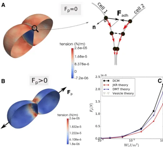
Fig. 2 a, b Cartoon of adhering
cell and detail of the force ele-ments acting in the cell surface triangulation. c Projection of a triangle pair ( T, T′ ) belonging
to different cells to compute the cell–cell interaction force
𝐅adh on a 2D plane for
illustra-tion. Note that in the (2D) projection, a triangle in 3D gives only two nodes, whereas the circumscribing spheres are represented as circles ( C, C′
) each with well defined radii.
d Simulation snapshot of
adhe-sion between a CBM and a deformable cell model (DCM). The color bar is according to membrane tension (see Eq. 8)
in DCM the interaction forces need to be defined for each node individually, thereby endowing representation of local surface heterogeneities. This can be achieved by pairwise potential functions (Van der Waals, Morse) between nodes which mimic the effect of short-range repulsion and
long-ranged attraction forces of molecules (Tamura et al. 2004;
Rejniak and Anderson 2008; Sandersius and Newman 2008;
Jamali et al. 2010). While straightforward to implement, this
approach poses some problems with respect to the scalability and calibration of the parameters for these potentials. Fur-thermore, pairwise potentials are not efficient in avoiding unwanted interpenetration of two approaching cells. The alternative approach followed in this work (which largely avoids these problems) is based on Maugis–Dugdale theory. This has been successfully applied to predict red blood cell
spreading dynamics on surfaces (Odenthal et al. 2013). The
Maugis–Dugdale theory for adhering bodies is a
generaliza-tion of the JKR theory for spheres (Maugis 1992). It
cap-tures the full range between the Derjaguin–Muller–Toporov (DMT) zone of long reaching adhesive forces of a soft homo-geneous isotropic elastic sphere and small adhesive deforma-tions of the Johnson–Kendall–Roberts (JKR) limit of a hard homogeneous isotropic elastic sphere of short interaction ranges. Here, we assign each triangle of the cell surface with a circumscribing sphere reflecting the local curvature. Two triangles belonging to different cells can interact by collision of their assigned spheres. To compute the magnitude of these interactions, we use Maugis–Dugdale stress formula.
In our model, Maugis–Dugdale theory is applied to a dis-crete system of triangles, which constitute the cell surface. This assumes a quasi-continuous distribution of cadherin
bonds at the cell contact area.4 Because the cell curvature
is not constant as it would be for a perfect sphere, we locally estimate the curvature from the triangulated structure (see
Fig. 2c) using the discretized Laplace–Beltrami operator,
which is an approximation function to associate a mean cur-vature vector to a discretized surface or boundary curve as an alternative to the approximation by the angle between the
surface normal vectors (Drasdo and Forgacs 2000). In this
way every triangle of the cell can be associated with a local curvature vector 𝐑i for which a circumscribing sphere can be defined. An interaction between two cells defines several pair-wise triangle–-triangle interactions ( T, T′ ). One pair of
trian-gles defines a pair of circumscribing spheres ( C, C′) with radii
determined by the curvatures, and a common contact plane to
which their triangles are projected (Fig. 2c, dashed red line).
The local stress at the contact, which depends on the radius of both spheres and the adhesion energy can then
be computed using the adhesive Maugis–Dugdale stress component:
In this formula, r is the distance from the contact point, a is the effective contact radius (pure Hertz contact) and c
is the radius of the adhesive zone (see Fig. 2, bottom). We
then compute the Tabor coefficient (Johnson and Greenwood
1997):
where ̂E and ̂R are the reduced elastic moduli and radius
of the two objects in contact.5 The tension 𝜎
0 is the
maxi-mum adhesive tension from a Lennard-Jones potential and
is related to the specific adhesion energy W by W = h0𝜎0 .
Here h0 is the typical effective adhesive range that reflects
the attractive cutoff distance between the bodies. We set
h0 = 2 × 10⁻⁸m in all the simulations (Leckband and
Israelachvili 2001; Odenthal et al. 2013). After this, c can
be computed from m = c∕a for which holds:
On the other hand, the repulsive part is given by the Hertz pressure:
The total stress distribution between the two spheres is thus pa+ pr . The total interaction force 𝐅adh,i+ 𝐅rep,i between a
pair of triangles is obtained by integrating this stress using standard Gauss quadrature rules over the surface area com-mon of the two triangles that have been projected on the contact plane. Once the force is known, it is distributed onto the nodes of both triangles, with the total force on the first triangle opposite in sign to the one of the second, to con-serve total momentum. Note that for each triangle which has a contact area A with another triangle, each node associated with this triangle acquires a contact area A / 3. For more
details about the implementation, see Odenthal et al. (2013)
and Smeets et al. (2014, 2019).
Importantly, this interaction model also permits to simu-late interactions between a triangusimu-lated body and a smooth
(14) pa= { −𝜎0 𝜋 arccos ( 2a2−c2−r2 c2−r2 ) if 0≤ r ≤ a −𝜎0 if a≤ r ≤ 0. (15) 𝜆 = 𝜎0 ( 9 ̂R 2𝜋W ̂E2 )1∕3 , (16) 𝜆 2 � 4a3Ê 3𝜋W ̂R2 �2∕3� (m2− 2) sec−1m+√m2− 1� +4𝜆 2 3 � 4a3Ê 3𝜋W ̂R2 �1∕3 � (m2− 2) sec−1m− m + 1�= 1. (17) pr= 2 ̂E 𝜋 ̂R √ a2− c2.
4 We assume here a constant and homogeneous adhesion field.
However experiments have pointed out that adhesion bounds are more point-like and can reinforce over time (Pawlizak et al. 2015). Although this consideration could be addressed with our model, it remains out of the scope of this paper.
5 ̂E is given a large value compared to the cell Young modulus to
surface such as spheres or planes having fixed curvature. In such case, the contact establishes simply between the sphere assigned to a triangle, and the sphere that represents the object as a whole. This allows to implement a relatively simple algorithm that defines the handshake between a DCM
and a CBM (see example Fig. 2d).
Cell migration force—term (9) in Eq. 1: The migration
force 𝐅mig is usually an active force, representing the random
micro-motility of a cell. Migration of cells involves complex mechanisms such as filopodia formation and cell contractil-ity, and may be modeled as such (see, e.g., Tozluoğlu et al.
2013; Kim et al. 2018), but for the sake of simplicity we do
not resolve the migration in such detail and instead lump the different mechanisms into one net force, which is homoge-neously distributed to the nodes the cell. For specific appli-cations, the forces might be in-homogeneously distributed. In the absence of influences that impose a certain direction or persistence, it is commonly assumed that the migration
force is stochastic, formally resulting in 𝐅mig= 𝐅ran , with
⟨𝐅ran⟩ = 𝟎 , and ⟨𝐅ran(t) ⊗ 𝐅ran(t�)⟩ = 𝐌𝛿(t − t�) , where
𝐌 is an amplitude 3 × 3 matrix and relates to the diffusion
tensor 𝐃 of the cell. As cell migration is active, depending on the local matrix density and orientation of matrix fib-ers, the autocorrelation amplitude matrix 𝐌 can a priori not be assumed to follow a fluctuation–dissipation (FD) theorem. However, “measuring” the position of a cell in the simulations the position autocorrelation function might be experimentally used to determine the diffusion tensor using
⟨((𝐫(t + 𝜏) − 𝐫(t)) ⊗ (𝐫(t + 𝜏) − 𝐫(t))⟩ = 6𝐃𝜏 , and 𝐌 be
calibrated such that the numerical solution of the equation of motion for the cell position reproduces the experimental result for the position autocorrelation function. For exam-ple, in a homogeneous environment 𝐌 can be casted into a
form formally equivalent to the FD theorem, leading to a kBT
-equivalent for cellular systems, that is controlled by the cell
itself (Van Liedekerke et al. 2015; Drasdo and Hoehme 2012).
On the other hand, if cells migrate in response to a morpho-gen gradient, an additional directed force 𝐅mor into the direction
of the concentration gradient of the morphogen may occur. The total migration force for the cell reads then 𝐅mig= 𝐅ran+ 𝐅mor .
In the liver lobule example simulations (Model III in Sect. 3.3), we assume that only “leader” cells have the capability of directed migration. These are the cells in the lobule that are located at the interface to the pericentral necrotic lesion.
Note finally, we assume here momentum transfer to the ECM by the ECM friction and active micro-motility term but we do not model the ECM explicitly.
2.1.2 Cell growth and mitosis
During progression in the cycle, a cell grows by acquiring dry mass and water, eventually doubling its volume. This
volume growth in both, interphase consisting of the G1 , S
and G2 phase, and mitosis phase may be described by an
increase in the radius of the cell. We assume here that for a cell in free suspension during growth stage, the reference
volume of the cell V0 gradually increases and is updated
according to:
where 𝛼 is the growth rate for simplicity assumed to be con-stant during the cycle, which can be justified if we look at timescales much larger than one cell division
(Van Liede-kerke et al. 2019). 𝛼 is chosen such that the volume of a cell
doubles in the experimentally observed cell cycle duration. Cell growth and division in the CBM (see, e.g., Drasdo
et al. 2007) is straightforward to implement, but involved for
the DCM, requiring a multistep procedure.
Cell growth: During cell growth, the volume of the cell
is increasing (Fig. 3a, b). We model this by an update of
the reference volume V0 following Eq. 11, update of the
(18) V0(t + Δt) = V0(t) + 𝛼Δt,
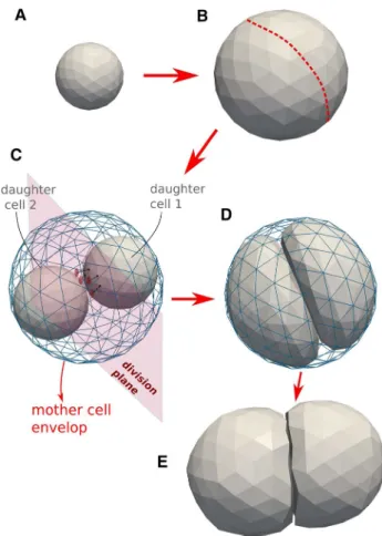
Fig. 3 Model algorithm of the cell cycle of deformable cells: a, b cell growth (double volume by increasing the radius). b Choose division direction randomly (assign nodes to one side). c Add two default cells as daughter cells to center of masses. Project nodes of the daughter cells to surface of division plane if they intersect it. A sub-simula-tion is run to come rapidly to situasub-simula-tion D. d After the sub-simulasub-simula-tion, mother envelope is removed. e Division stage finished: two mechani-cally relaxed daughter cells
reference values of the cell surface triangle areas, and
update of the spring lengths. The reference triangle area A0
for each triangle, and spring rest length l0 for each
viscoelas-tic element are recomputed every time step Δt according to A0(V0(t + Δt)∕V0)2∕3 and l
0(V0(t + Δt)∕V0)1∕3 , respectively.
The coordinated update of V0 , A0 and l0 in the algorithmic
implementation of the model is necessary to ensure that no additional volume penalty forces or other artifacts are gener-ated during growth. Note that at this moment, growth inhibi-tion due to excessive external mechanical stress (e.g., Drasdo
and Hoehme 2012) can be easily included in our model, but
in the scope of this paper we do not consider it further. Cell death: When a cell dies, it can be either removed instantly from the simulation, or gradually shrink (lysis). Algorithmwise, lysis can be regarded as the inverse of the growth process. However, during lysis the mechanical parameters of the cell may change. The process may con-tinue until a certain cell volume has been reached, below which the cell cannot longer shrink. Finally, a lysed cell may be removed completely from the simulation (e.g., by phagocytosis).
Cell division: During cytokinesis, the continuous shrink-ing of the contractile rshrink-ing, together with the separation of the mitotic spindle, gradually creates the new daughter cells. After mitosis the cell has split up in two adhering daughter cells. An analytical approach describing this process can be
found in Turlier et al. (2014). An approach with 2D
deform-able cells has been previously proposed (e.g., Jamali et al.
2010). In a first attempt, we had implemented such an
algo-rithm in 3D but this turned out to be prone to numerical instabilities, as triangles on the side of the contractile ring tended to be extremely stretched while nodes accumulated at the position of the contractile ring. Hence, simulations of these processes in DCM in 3D would require a complex re-meshing process for the surface to leave the local stresses unchanged but avoiding numerical instabilities. An imple-mentation of these steps turned out to be not only challeng-ing, but also computationally time consuming.
As we are merely interested in long-term effects (i.e., several hundreds of cell divisions), and as the cytokinesis is a short process compared to the duration of the entire cell cycle, we avoid these particular tedious intermediate steps in our model, and instead directly create two new adhering cells that are enclosed by the mother cell just before its divi-sion as pictured in Fig. 3.
First, a division plane is chosen, which determines the direction into which the cells divide. The label of the divi-sion plane on the surface of the mother cell can be associ-ated with the position of the contractile ring. The orientation of this plane may be chosen randomly or into a preferred direction, and splits the mother cells into two halves each bounded by part of the surface of the mother cell and the
division plane (see Fig.3b, c); note that the mother cell in
the figure is spherically shaped, but the algorithm works for arbitrary cell shapes as well). Then, the centers of the two future daughter cells on both sides of the plane are computed as the two centers of mass of the nodes that form each of the two halves, and each of those two centers of mass is associ-ated with the center of a new spherically shaped daughter
cell (Fig. 3c). The radii of the daughter cells are chosen such
that they are both contained by the mother cell. To ensure the daughter cells are not overlapping at this stage, those nodes that would overlap with the division plane are pro-jected back on the division plane. Each of the daughter cells has now as border approximately a half of the mother cell envelop and the division plane that it shares with the other daughter cell. At this stage however, the radii (and volumes) of the daughter cells are not yet those they each should have, i.e., half of the volume of the mother cell.
To achieve this, a sub-simulation6 is performed where the
cell volume and strut lengths of the viscoelastic network are reset to their reference values for a cell half the size of the mother cell. During the sub-simulation, we artificially set all friction coefficients of the daughter cells to very small values. This “inflates” the two daughter cells rapidly. On the other hand, we momentarily freeze the positions of the nodes of the mother cell. As a consequence, the two cells will rapidly adapt their shapes to the limiting shape of the mother cell “cocoon” and the division plane. The repelling interactions between the triangulated envelop of the mother cell and daughter cells ensure that the latter stay inside. We thus arrive in this step at a system of three triangulated cells: one fixed mother cell, and two encapsulated daughter cells with forming a shape approximately that of mother cell just before cell division.
After the sub-simulation, all the friction coefficients are reset to their normal values, the division plane is discarded and the daughter cells start adhering to each other because the mutual adhesion forces are invoked. The mother cell envelop is removed from the simulation and the daughter cells interact again with their environment. The system can
relax slowly toward a mechanical equilibrium (Fig. 3d) over
a time span equal to the mitosis phase duration.
2.2 Center‑based model (CBM)
Center-based models (CBM) are well-established modeling approaches where cells have the same features as in DCM, but the cell shape is approximated as a simple geometrical object. The cell shape is not explicitly modeled but only captured in a statistical sense. The cells are represented by
homogeneous elastic and adhesive spheres (see Fig. 1a,
bot-tom), and interact through pairwise forces (e.g., Hertz, JKR),
6 A sub-simulation means that it runs in parallel and does not add up
to the total simulation time (time is kept constant). The duration of a sub-simulation is very short, of the order of 10 s.
which are computed from a virtual overlap of both cell geom-etries. The equation of motion is similar to that of DCMs, yet the forces are here directly applied to the cell centers
(for details, see Sect. 2.3). During division, two new cells
are created next to each other that replace the mother cell. In our work, we will use the CBM for comparative runs in the simulations for liver lobule regeneration (Hoehme et al.
2010), see Sect. 3.3.
2.3 Forces, equations of motion and cell division
We here only briefly recapitulate the basic components of CBM: for more detailed information, we refer to literature (see,
e.g., Drasdo and Höhme 2005; Drasdo and Hoehme 2012; Van
Liedekerke et al. 2015). In CBM, cells are usually represented
as spheres. The equation of motion for a cell i reads:
For the same reasons as for the DCM, inertia is neglected as cell movement occurs. The first term on the lhs. denotes the friction of cells with the substrate or extracellular matrix, the second term cell–cell and—in simulations of the regen-erating liver lobule as explained in the introduction of this paper—cell-sinusoid friction forces. Sinusoids are modeled in this work as immobile chain of slightly deformable
spheres (hence 𝐯j= 0 for sinusoidal elements j) with the
radius equal to the sinusoidal radius found experimentally
(Hammad et al. 2014). For cell–cell friction, the velocities
𝐯j will generally be not zero. 𝐅int
ij denotes interaction forces
on cell i from repulsion or adhesion with other cells j or
static blood vessel cells (see Sect. 3.3). The force 𝐅sub
i reflects adhesive/repulsive interactions with a flat substrate or wall. 𝐅mig
i denotes the total migration force which has a
random part and may also have a directed term (see explana-tion DCM). The fricexplana-tion terms involve tensors for the cell–cell friction ( 𝚪cc
ij ) and cell–substrate friction ( 𝚪
cs
i ). The friction tensors are computed in the same way as for the DCM, with the nodes of the DCM being replaced by the
actual cell centers in the CBM (Drasdo and Hoehme 2012).
The cells in CBM interact by pairwise forces having a repulsive and adhesive part, which are characterized by a
function of the geometrical overlap 𝛿ij= Ri+ Rj − dij . As in
Chu et al. (2005), we assume here that cell adhesion forces
can be described by Johnson–Kendal–Roberts (JKR) model, approximating cells by isotropic homogeneous sticky elastic bodies that are moderately deformed if pressed against each other. The interaction force is computed by
(19) 𝚪csi 𝐯i+ ∑ j 𝚪ccij(𝐯i− 𝐯j) =∑ j 𝐅intij + 𝐅subi + 𝐅 mig i (20) Fintij = 4 ̂E 3 ̂R [ a(𝛿ij)]3− √ 8𝜋W ̂E[a(𝛿ij)]3.
The contact radius a in Eq. 20 allows to compute the
cell–cell contact area, and can be obtained from Pathmana-than et al. (2009):
In the latter equations, ̂E and ̂R are defined as
with Ei and Ej being the Young’s moduli, 𝜈i and 𝜈j the Pois-son numbers and Ri and Rj the radii of the cells i and j,
respectively. W = ρm Wb is the specific surface
adhe-sion energy obtained by multiplying the surface density of
adhesion molecules ρm with the adhesion energy Wb stored
in a single adhesive bond. Note that the Young moduli in the center-based model should be chosen such that they cor-respond as much as possible to the elastic properties of the DCM. In particular, we warrant here that for a CBM’s Young
modulus and Poisson’s ratio, E = KV∕3(1 − 2𝜈) where KV
is the compression modulus of the DCM cell (Sect. 2.1).
Note that for a CBM, the elastic properties of the cortex and membrane cannot be identified a priori.
During the cycle the intrinsic volume of a mother cell doubles before it splits into two daughter cells. The intrin-sic volume is defined by the volume of the cell if it would be undeformed and uncompressed. Its true volume in case it interacts with other cells or structures cannot be exactly tracked as the CBM does mostly not permit to calculate the volume of cells interacting with other cells. Like in the DCM, we are assuming constant growth rate during the cell cycle and the intrinsic volume Vi of cell i is updated
every time step Δt as in Eq. 18.
If the cell passed a critical volume Vcrit , the cell
under-goes mitosis and two new cells with volume Vcrit∕2 are
created. In case the cell grows to twice its original value to
divide as considered throughout this work, Vcrit = 2V0. A
simple version of the division algorithm consists of plac-ing directly two smaller daughter cells in the space origi-nally filled by the mother cell at the end of the interphase
(Schaller and Meyer-Hermann 2005; Galle et al. 2005).
When the two daughter cells are created, the JKR inter-action force will push away the two daughter cells until mechanical equilibrium is reached. If the space filled by the mother cell is small, which is often the case for cells in the interior of a cell population, the local interaction forces occurring after replacing the mother cell by two spherical daughters can adopt large (unphysiological) values leading to unrealistic large cell displacements. This might be cir-cumvented by intermediately reducing the forces between the daughter cells (see below). Alternatively, cells could (21) 𝛿ij= a2 ̂R − √ 2𝜋W ̂ E a. ̂ E= ( 1− 𝜈2 i Ei + 1− 𝜈2 j Ej )−1 and ̂R= ( 1 Ri + 1 Rj )−1 ,
in small steps be deformed during cytokinesis into
dumb-bells before splitting (Hoehme et al. 2010). In this work,
we pursue the simpler approach as it resembles the cell division algorithm we use for the DCM.
2.3.1 Corrections to JKR contact forces
As mentioned above, center-based models suffer from a number of major artefacts, often ignored in simulations.
The most striking is that common pairwise contact forces (type Hertz, JKR, etc.) and contact areas become largely inac-curate when cells are densely packed and become jammed and compressed. This problem discussed in Van Liedekerke et al. (2015); Van Liedekerke et al. (2019) is comparable to the pack-ing problem in liquid foams and emulsions as described in
Höhler and Weaire (2018), Höhler and Cohen-Addad (2017).
In densely packed cell aggregates, the deformation a cell, say cell i, experiences as a consequence of interaction with one of its neighbors, say cell j can be so large, that it affects the interaction cell i has with another neighbor cell, say cell k ≠ j . In that case the approximation of considering the interaction forces between the pair cell i and cell j as independent of the interaction force between the pair cell i and cell j becomes inaccurate. As a consequence, even an incompressible cell characterized by Poisson ratio 𝜈 = 0.5 in the JKR force model
(Eq. 20) will be compressed if surrounding cells are pushed
toward it. In such a situation, cell volume and cell–cell contact area are only poorly approximated by the JKR force model.
Voronoi tessellation of the positions of the cells can esti-mate the individual cell volumes (and hence predict realistic
pressure forces) (Bock et al. 2010; Schaller and
Meyer-Her-mann 2005). However, in the attempt to correct the
unrealis-tic contact forces in the center-based model upon large com-pression forces, we here propose a simple calibration step in which we use DCM simulations to estimate contact forces between cells. The DCM does not have the aforementioned problem because the shape and cell volume are determined at high spatial and temporal resolution. As such, there is no notion of geometrical overlap in DCM cells. A small clump of DCM cells is compressed quasi-statically while monitor-ing the contact forces as function of the distances between
the cell centers (see “Appendix 1”, Fig. 12b). During
com-pression, a stiffening of the contacts can be clearly observed. Performing an equivalent experiment with CBM using the JKR law results in a significant underestimation of the
con-tact forces (Fig. 12b). To correct these, we partially follow
the procedure as outlined in Van Liedekerke et al. (2019). As
in this work, we keep the original JKR contact law form but
modify the apparent modulus Ei→ ̃Ei of the cell as the cells
approach each other, by gradually increasing it in Eq. 20 as
the cells get more packed. The challenge lies in determining ̃
Ei as a function of the compactness of the spheroid. We try to estimate the degree of packing around one cell by using the
distances between that cell and its neighbors, introducing a function that depends on the local average of the distances ̃di=
∑
j̃dij∕N (with ̃dij= 1 − dij∕(Ri+ Rj) and N is the total
number of contacts7) to each of the contacting cells j, noticing
that the cell–cell distances differ only very slightly. We here considered the case where all cells all have the same elastic modulus; for interacting cells of different parameters, the pro-cedure might have to be adapted. Different to Van Liedekerke
et al. (2019) we do not take into account the effective volume
reduction of the CBM cells, because we assume that cells are not as heavily compressed. The simulated force curves of the DCM could well be reproduced with the CBM for the follow-ing simple polynomial function of 4th order:
in where a0= Ei and, a1 is a fitting constant. The best
fit to the DCM contact force is shown in Fig. 12a, with
a1 = 4 × 10⁶ . However, we note that the contact stiffness
generally depends on the number of neighbors a cell has. In this experiment, every cell had initially 8 contacting neigh-bors, yet this number evolves to approximately 12 as the compression progresses, which is what would be expected from the Euler theorem for volume tessellation.
A side effect of this calibration method is that high repul-sive forces may arise during cell division, when two new cells are created and positioned close to each other. To limit these effects, we apply the above formula in a such way, that the con-tact stiffness becomes gradually larger over a time period just after division, which we choose about ∼ 1∕10 of the cell cycle (roughly the duration of mitosis phase; however, smaller dura-tions would also be possible), reaching the maximal value after this period. This is similar as what has been used in Galle et al. (2005) to avoid repulsion force cues, and ensures that cells will not separate abruptly during division. The period gives time to the cells to evolve to a local mechanical equilibrium, and can be seen as the analog of the relaxation period in the division
algorithm in the deformable cell model (see Sect. 2.1.2). We
have verified that small variations on this relaxation period did not influence the simulations results significantly.
3 Results
3.1 Single cell experiments
3.1.1 Calibration of DCM parameters from optical stretcher experiments
Classical experiments such as optical stretchers, optical tweezers, and micro-pipetting techniques are used to observe (22) ̃
Ei( ̃di) = a0+ a1̃di4,
7 Note that ̃d
ij would correspond to the sphere-sphere overlap in the standard CBM.
the mechanical behavior of individual cells and can be used to estimate the physical range of the DCM viscoelastic
network model parameters (see, e.g., Odenthal et al. 2013;
Guyot et al. 2016; Fedosov et al. 2011). Here, we choose the
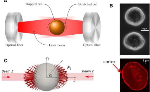
optical stretcher experiment where, as the experiment is per-formed in suspension, represents a type of ground state and thus an excellent situation for the calibration of the mechani-cal parameters. Therefore, the optimechani-cal stretcher experiment is mimicked in silico with a DCM. In the optical stretcher, two laser beams in opposite direction and faced to each other trap
a cell in suspension (see Fig. 4a). The diffracted laser beams
exert a surface force on the cell’s membrane and cortex, deforming it toward the beam direction. Increasing the laser power yields a higher optical stretching force. At the same time, the deformation along two perpendicular directions is measured using image analysis, yielding information on
cell shape. We refer to Guck et al. (2001, 2005) and Grosser
et al. (2015) for more details of the setup and conditions in
such an experiment.
New data of optical stretcher experiment were generated using MDA-MB-231 breast cancer cells. These cells had an average radius of 8.8 ± 1.3 μm ( N = 100 samples). Actin staining further revealed average approximate cortex
thick-ness of hcor∼ 500nm (Fig. 4b).
In each experiment, the laser beams were applied during a time interval of a few seconds, in which the cell continues to deform. Thereafter, the cell relaxation behavior period was monitored for several seconds. The long axis (Z) and short axis (Y) lengths changes over time are derived from
analyzing the images (see data Fig. 5; the X-axis and Y-axis
are by rotation symmetry with regard to the Z-axis assumed to be equally long). Two laser powers were considered
( P0= 900 mW and P0= 1100 mW ), with an applied
stretch-ing time of two seconds and a monitorstretch-ing of the relaxation
behavior of two seconds. Because of the large biological variability, for each individual experiment the measurement has been taken with a minimum of about 100 cells.
In a first step, we identified some parameters and/or their ranges by comparison to published references.
An initial spherical deformable cell was created with a total of N = 642 nodes (test runs indicated that further spa-tial refinement was not required). The cells were immersed in a medium with viscosity 𝜇 being close to that one of water. We approximate the cell-medium friction coefficients
for each note needed to determine term (3) in Eq. (1) by
𝛾ns= 𝛾liq∕N = 6𝜋𝜇R∕N . This approximation ensures that
for a spherical cell of radius Rc modeled by N nodes at its
surface, the friction coefficient is precisely as predicted by the Stokes equation.
Determination of the force terms (4) and (5) in Eq. 1
requires determination of the elastic modulus of the cell cortex. Because we did not have information on the elas-tic properties of the MDA-MB-231 cells, we adopted a nominal value for the elastic modulus of the cell cortex
Ecor ∼ 1 kPa based on different cell types (see Tinevez
et al. 2009; Brugués et al. 2010). Applying Eqs. 7 and
10, which relate the elastic moduli to the parameters of
the coarse-grained model of the CSK, the nominal cortical
stiffness constants in the model are thus ks∼ 4 × 10⁻⁴N∕m ,
kb∼ 1 × 10⁻¹⁷N/m (see Sect. 2.1, Eqs. 3 and 10). To
deter-mine the compression force of the cell represented by
term (6) in Eq. (1), we need to know the cell compression
modulus KV , which is still subject of debate. For instance,
Delarue et al. (2014a, b) conclude from experiments with
growing spheroids under pressure that cells are compress-ible with compression moduli of the order of 10 kPa. On
the other hand, the Monnier et al. (2016) find individual cell
compression moduli of several orders of magnitude higher
Fig. 4 a Sketch of the
experi-mental setup with a trapped cell in an optical stretcher. b Top: image of unstretched and stretched MDA-MB-231 cell. Bottom: actin-stained image of a MDA-MB-231 cell indicating cell cortex actin cytoskeleton.
c Surface forces profile due to
laser is visualized (red arrows) on a triangulated surface of the deformable cell. The Z-axis (long axis) is aligned with the laser beam, whereas the X- and the Y-axis give the direction of the short axes during defor-mation. 𝐅L is the nodal force
(1 MPa) than the one reported above. Yet, Monnier et al. have measured this over short time period and accordingly they further state in their paper that on longer timescales, the compression modulus might differ from that value may due to adaptation of the cell. In the work of Tinevez et al.
(2009), the cytoplasm compression modulus is estimated as
± 2500 Pa. Although this is not the compression modulus
of the whole cell, it indicates that if cells are able to expel water through the aquaporins on longer timescales, this may
be a good estimate of KV . We here adopted this value but we
note that in the simulations for the optical stretcher, we did not find any significant influence on the results during the
time course of the experiment when KV was varied within
100 Pa to 10000 Pa , see “Appendix 2”.
Term (7) of Eq. (1) represents the effect of bilayer
com-pression modulus KA (see Eq. 12). For pure lipid bilayers,
about 0.2 N∕m has been reported, while in case of a plasma membrane of a cell, much lower values have been measured,
Fig. 5 a, b Comparison of
the simulated MDA-MB-231 cell deformation with the experimental data in an optical stretcher, using laser powers of 900 mW and 1100 mW . a The model was first fitted using a Kelvin–Voigt model (KVE) and assuming temperature dependent friction coefficients for the cytoskeleton. b The model then was fitted assum-ing a modified Maxwell model (MME) but using the same temperature dependence as for KVE. For sake of clarity, the error bars are only shown for some data points, and only for the P0= 1100 mW case. The
errors bars on the data are quite large, indicating a high biologi-cal variability. c Temperature dependence of damping coef-ficients, using model fit for DCM, compared to Arrhenius’ law using an activation energy close to the value reported in Kießling et al. (2013). d Sche-matic representation of nodal force elements with springs and dampers. KVE, Kelvin–Voigt element; ME, Maxwell element; MME, modified Maxwell ele-ment