Towards bridging the gap between reprensentation and formalism in the context of systems life cycle management processes

Faculté des Sciences Economiques Avenue du 1er-Mars 26

CH-2000 Neuchâtel

www.unine.ch/seco

PhD Thesis submitted to the Faculty of Economics and Business Information Management Institute

University of Neuchâtel

For the degree of PhD in Computer Science by

Eric SIMON

Accepted by the dissertation committee:

Prof Kilian Stoffel, University of Neuchâtel, thesis director Prof Valéry Bezençon, University of Neuchâtel, president of the jury

Dr Paul Cotofrei, University of Neuchâtel Dr Thibault Estier, University of Lausanne

Dr Willy Picard, Poznan University of Economics, Poland

Defended on 11 December 2013

TOWARDS BRIDGING THE GAP BETWEEN

REPRESENTATION AND FORMALISM IN THE CONTEXT OF

SYSTEMS LIFE CYCLE MANAGEMENT PROCESSES

Summary

In the context of systems development life cycles (SDLC), a gap exists between the representations of the involved methodologies as process on the one hand, for example using business process model and notation (BPMN), and the formalisms that would provide the level of analysability necessary to validate the corresponding processes on the other hand beyond mere ex-ecution, for instance Petri nets. This doctoral thesis aims at bridging this gap by proposing a model in-between these two extremes that is simple yet expressive enough to be able to represent the processes, either directly or by translating BPMN diagrams to the model, while retaining enough form-alism to allow its mapping to Petri nets, which enables the execution of the diagrams but also opens the door to automatic or semi-automatic val-idation of some properties of the systems using well-known algorithms in graph theory or methods that are specific to Petri nets. The model consists in a graphical extension of finite state automata theory, allowing synchron-isation and composition of sub-processes. The model is then translated to the corresponding Petri net for execution. A further mapping, from BPMN diagrams to the model, allows a structural analysis of the described pro-cesses. Practical examples illustrate some of the possibilities and limitations of the approach, and open the discussion about possible future theoretical or practical research around these ideas.

BPMN.

Résumé

Dans le contexte de la gestion des cycles de vie des systèmes (SDLC), on ob-serve un fossé entre, d’une part, les représentations utilisées pour modéliser les méthodologies sous forme de processus, par exemple en utilisant business process model and notation (BPMN), et d’autre part les formalismes qui of-friraient les possibilités d’analyses nécessaires à la validation des processus correspondants, comme par exemple les réseaux de Petri. Cette thèse de doc-torat vise à combler ce fossé en proposant un modèle quelque part entre ces deux extrêmes qui soit à la fois suffisamment simple et expressif pour re-présenter les processus, soit directement, soit en traduisant les diagrammes BPMN dans ce modèle, tout en conservant un niveau de formalisme suffi-sant pour permettre sa traduction dans des réseaux de Petri, ce qui permet également l’exécution des diagrammes, mais ouvre en outre la porte vers la validation automatique ou semi-automatique de certaines propriétés des systèmes en utilisant des algorithmes connus en théorie des graphes ou des méthodes propres aux réseaux de Petri. Le modèle consiste en une extension de la théorie des automates à états finis permettant la synchronisation et la composition de sous-processus. Le modèle est ensuite traduit dans le réseau de Petri correspondant pour exécution. Une correspondance supplémentaire, cette fois de diagrammes BPMN vers le modèle, permet une analyse structu-relle des processus décrits. Des exemples pratiques illustrent quelques-unes des possibilités et limitations que présente cette approche, et ouvrent la dis-cussion vers de possibles futures recherches théoriques ou pratiques liées à ces idées.

A Ph.D. thesis is often seen as a lonely progression towards some elusive goal. But no such adventure could be undertaken without the contribution and presence of many different people.

First, I would like to thank Kilian, for hiring me as his assistant many years ago, and for believing in me. My thanks also to Paul, for his scientific guidance, and for his friendship. I shall also remember my former office mates and colleagues Gina, Claudia, Iulian, Thorsten, Christophe, Marcelo, Dong, Tudor and Fabrizio, for the joyful atmosphere, the lunches, and the philo-sophical discussions we had with each other.

The work was made possible by the generous funding of both the Uni-versity of Neuchâtel, and the Hasler Foundation. I am very grateful to these institutions.

A very special thought goes to my parents, and to Eléonore, for their moral support, their encouragements, and their understanding over the past several years.

1 Introduction . . . 1

2 Preliminaries . . . 7

2.1 The Systems Development Life Cycle . . . 7

2.1.1 A Bit of History . . . 7

2.1.2 Towards Formalisation . . . 14

2.2 Finite State Automata . . . 16

2.3 Business Process Model and Notation . . . 17

2.4 Petri Nets . . . 24 2.5 Social Protocols . . . 27 3 The Model . . . 29 3.1 Argument . . . 29 3.2 Synchronisation . . . 32 3.3 Components . . . 34 3.4 Formal Definition . . . 35

3.5 Mapping the Model to Petri Nets . . . 38

3.5.1 Synchronisation . . . 38

3.5.2 Composition . . . 40

4 Application to SLCM . . . 43

4.1 Introduction . . . 43

4.2 Modelling the Processes . . . 45

4.3 Adding Concurrent Activities . . . 52

4.4 Discussion . . . 56

4.4.1 Detection of Graphical Errors . . . 56

4.4.2 Detection of Cycles . . . 58

4.4.3 Detection of Badly Constrained Alternatives . . . 60

4.4.4 Advantages over Other Representations . . . 61

5 Application to BPMN . . . 63

5.1 Mapping BPMN to the Model . . . 65 I

5.2.2 Creation of a new educational programme . . . 76

5.2.3 Implementation of a new educational programme . . 80

5.2.4 Update of an existing educational programme . . . . 83

5.3 Summary . . . 89

6 Conclusion and Future Work . . . 91

A The Prototype . . . 97

B Parser Specifications . . . 103

Bibliography . . . 114

List of Figures

2.1 The two steps of the software development process . . . 8

2.2 The seven phases of the waterfall model . . . 8

2.3 The phases of Royce’s final model . . . 9

2.4 Royce’s Waterfall Model . . . 10

2.5 _{Hermes 2003 . . . .} 11

2.6 _{Hermes 5 . . . .} 12

2.7 The V-Model . . . 12

2.8 The ten steps of the SDLC . . . 15

2.9 Representation of finite state automata . . . 17

2.10 Representation of BPMN diagrams: an example . . . 23

2.11 Representation of Petri nets . . . 26

3.1 The mechanism of synchronisation in the model . . . 33

3.2 The representation of an alternative in finite state automata theory . . . 33

3.3 The mechanism of composition in the model . . . 37

3.4 The mapping, or translation, of a FSM to a Petri net. . . 39

3.5 Mapping the synchronisation to Petri nets . . . 39 II

4.1 ISO 12207 The relationship of primary life cycle processes and

roles . . . 44

4.2 ISO 12207 5.1.1 . . . 47

4.3 ISO 12207 5.1.2 with a custom process . . . 48

4.4 ISO 12207 5.1.3 . . . 48

4.5 ISO 12207 5.1.4 . . . 49

4.6 ISO 12207 5.1 complete version (engine) . . . 50

4.7 ISO 12207 5.1 complete version (Petri net) . . . 51

4.8 ISO 12207 5.1.3.5 and synchronisation . . . 53

4.9 ISO 12207 5.1 with synchronisation (editor) . . . 54

4.10 ISO 12207 5.1 with synchronisation (engine, Petri net) . . . 55

4.11 SDLC Detection of graphical mistakes . . . 57

4.12 SDLC Detection of simple cycle . . . 58

4.13 SDLC Detection of synchronisation mistake with a cycle . . 59

4.14 SDLC Detection of badly constrained alternatives . . . 60

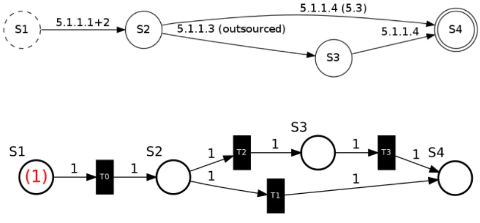
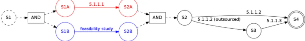
5.1 Towards filling the gap, first steps . . . 64

5.2 BPMN Events mapped to the model . . . 66

5.3 BPMN Task mapped to the model . . . 66

5.4 BPMN intermediate error event attached to the boundary of an activity, mapped to the model . . . 67

5.5 BPMN Exclusive gateway mapped to the model . . . 67

5.6 BPMN Parallel gateway mapped to the model . . . 68

5.7 BPMN Message flows mapped to the model . . . 69

5.8 BPMN Inclusive gateway mapped to the model . . . 70

5.9 BPMN Complex gateway mapped to the model . . . 70

5.10 BPMN choreography diagram mapped to the model . . . 71

5.11 BPMN ex: Student course registration . . . 74

5.12 BPMN ex: Model corresponding to Figure 5.11 . . . 75

5.13 BPMN ex: Creation of a new educational programme . . . . 77

5.14 BPMN ex: Model corresponding to Figure 5.13 . . . 78

5.15 BPMN ex: Model corresponding to Figure 5.13 (final states) 79 5.16 BPMN ex: Implementation of a new educational programme 81 5.17 BPMN ex: Model corresponding to Figure 5.16 . . . 82

5.18 BPMN ex: Update of an existing educational programme . . 85

5.19 BPMN ex: Model corresponding to Figure 5.18 . . . 86

5.20 BPMN ex: Graphical error in Figure 5.18 . . . 87

5.21 BPMN ex: Model corresponding to Figure 5.18 (corrected) . 88

A.1 Architecture of the prototype . . . 98

A.2 Screenshot of the editor (model) . . . 99

A.3 Screenshot of the simulator . . . 99

A.4 Screenshot of the editor (BPMN) . . . 100

A.5 Screenshot of the simulator . . . 101

List of Tables

Introduction

In the context of systems life cycle management (SLCM), a clear gap exists between the methodologies devised to manage the development or business processes on the one hand, and the formalisms available to represent and analyse the involved processes on the other hand.

On the first side, concerned with management, the methodologies that are applied throughout the entire life cycle of a system are meant to guide managers and development teams during the successive phases of the project, rather than to guarantee a predefined, fail-proof process. They provide clear decision points, measures and guidelines to facilitate management activities such as governance, regulatory compliance, planning, budgeting and report-ing.

But the methodologies are meant to be read and interpreted, not valid-ated or executed. They are informal.

Some do look very formal, especially those based on the philosophy of “big design up front”. The waterfall model [50] is certainly the most famous among such proposals, and it is still at the roots of some modern project man-agement methods, although it has long been criticised for its linear nature, which it not suitable for software development, because of the essential qual-ities and complexity of the involved processes [10].

Other attempts take into account the iterative nature of software devel-opment, like the spiral model [7], or are based on adaptive models, like rapid application development (RAD) [26], and the many methods grouped under the general denomination of “agile” [4]. Lately, hermes 5 [60] (Figure 2.6), the latest version of the Swiss IT project management method, incorporated these ideas as well by simplifying itself to the extreme, but the more in-formal the methodology, the more subject to interpretation it becomes. This is arguably a good thing for developers, and to some degree also to project

managers, but it causes the whole process to become very difficult – if not impossible – to describe, let alone to validate.

On the second side, concerned with the technical aspects of software in particular, and of systems in general, well-established formalisms exist to model the essential properties of both the actual software systems and the processes involved to produce and maintain them, or at least some of their

key features1_{. In addition to the representation itself, sound mathematical}

foundations give the possibility to validate properties and to do correctness proofs, under certain assumptions or restrictions inherent to the object under scrutiny.

Well-known examples of interest here are automata theory in general, and the theory of virtual finite state machines and event driven finite state machines in particular. These theories allow the execution of a software spe-cification from a formal representation. These techniques are often applied to develop safety critical applications or control software. In the same domain, Petri nets [35] are routinely applied to represent and analyse concurrent or real time systems, in order to ensure a high level of reliability. They have been applied to work flow validation as well [63, 64, 67, 41]. Even more ab-stract systems could be applied to do model checking, like µ-calculus [15].

Still in the context of safety critical applications in particular, and soft-ware systems with strong reliability requirements in general, such as em-bedded systems for example, other formalisms were developed, often with accompanying tool kits, like the Vienna Development Method (VDM), and its specification language VDM-SL and later VDM++ [6], Raise, i.e. Rigor-ous Approach to Industrial Software Engineering [47] and its specification language: the Raise Specification Language (RSL) [46] or the B-Method [1], derived from Z notation [2], now an ISO standard (ISO/IEC 13568:2002). Theories based on first-order logic have been appearing in publications as well [25].

But although these representations have value in the technical world, they are of limited use in the management world, i.e. in the context of software life cycle management. They can be applied, but they are often ill-suited for the task, having been built for other purposes and communities of users. Simply put, they seem to be too complex to cope with in the context of process work flows in the large.

The world of management developed its own representations of processes, like the Business Processes Model and Notation (BPMN), now in its second

1_{Here, a system is one possible outcome of a process, most notably a software or IT}

system. A process is the set of activities used to develop, maintain and decomission a system or to achieve any other outcome.

incarnation [58]. But BPMN, the most favoured representation, lacks the mathematical foundations necessary for the validation of properties such as those available in formal models like those mentioned above. It is essentially graphical in nature, not mathematical. It is aimed at communication, not validation, like other process notations [13].

There lies the essence of the gap between these two worlds. One side is technical, concerned with the representation and validation of properties in a well defined scope, while the other side is managerial, and although it has a long tradition of using graphical representations of all sorts, these are always aimed at people, which means they are far too fuzzy or informal to allow any automatic or semi-automatic validation.

In other words, nothing seems to exist to formalise the actual processes involved in the life cycle of systems with sound mathematical properties, allowing automatic or at least semi automatic validation, while at the same time being simple enough to use as a graphical representation in the mana-gerial community.

A few steps towards formalisation have been taken by large organisations or administrations, which are the first to suffer from this gap, their business processes and regulations being their very nature. Documents such as the US Department of Justice’s definition of SDLC or the ISO/IEC 12207 Standard for Information Technology for Systems Life Cycle Management (SLCM) [22] are among such attempts. These standards suffer from two main disadvant-ages resulting from their sheer complexity: first, they are very difficult to follow to the letter as such, even when accompanied by complete check lists, as is the case in the standardisation business, which somehow defeats their very purpose as tools for regulatory compliance; and second, they are very difficult, if not impossible, to validate or even to verify.

The idea presented in this thesis is to take one step further in bridging the gap between the methodologies and managerial representations on one side, with special consideration to the special case of BPMN, and the math-ematical models for validation on the other side, in particular Petri nets. This gap is represented in Figure 1.1, where the relevant models are plot-ted in relation to two dimensions: their level of simplicity, and their level of analysability, as it can be understood from the above discussion.

To achieve this goal, the first step was to provide managers, or any other non technical stakeholder, with a very simple representation providing the bare minimum for a graphical representation of processes. This first model was inspired by previous research conducted in the domain of Picard’s social protocols [36] and is described in Chapter 2. The idea was to somehow enforce a systems thinking approach to problem solving, something that is routine

simplicity analysability BPMN Petri nets FSA

GAP!

Figure 1.1 – A diagram showing the gap between several representations used in the two worlds (management and technical), with respect to the two dimen-sions: simplicity, and analysability, i.e. the provided system property validation possibilities. Note that SLCM is absent, as it is clear that it can be represented as BPMN, which can be seen as the frontier of the management world towards formalisation in this context.

in the technical world, but not usually emphasised on the managerial side. The second step was to show that this model, although itself lacking the mathematical properties necessary to allow validation, could nevertheless be mapped to a well-established mathematical representation with the necessary properties, in this case Petri nets [35].

The third and final step was to show that BPMN could be mapped to our model, with some restrictions, thus effectively bridging the gap in Fig-ure 1.1, under certain conditions. This permits, for example a pFig-urely graph-ical exploration and validation of the representations, the model being much simpler than BPMN in terms of the number of elements. Furthermore, the model is a very promising direction for semi-automatic analysis or valida-tion, since all the algorithmic proofs or analysis techniques applicable on Petri nets can potentially be applied.

This thesis is laid out as follows: First, Chapter 2 presents the founda-tions on which the research is based: software development life cycle (SDLC), business process model and notation (BPMN), finite state automata theory (FSA), Petri nets, and Picard’s social protocols [36]. Second, the model is presented in Chapter 3, in the form under which it was published in [51], together with its mapping to Petri nets, as was proposed later in [52, 53]. Those two proposals with their associated publications constitute the first

two contributions to bridging our gap. Chapter 4 shows a first example of application in the context of SDLC, using the prototype that was developed to validate the model and its mapping to Petri nets, prototype which is described in Appendix A. Then, a mapping of a subset of BPMN to our model is described as well, which constitutes the third contribution of this research. Four examples of application to real world work flows are presented and discussed in Chapter 5. This last part is the result of a joint effort with Paul Cotofrei in the context of the research funded by the Hasler Foundation (see Acknowledgements). Further research by Cotofrei was conducted to ac-tually go one step further in this context by automatically infering business processes diagrams from legal or regulatory documents. This closely related research was published in “Business Process Modelling for Academic Vir-tual Organizations” [12]. Finally, possible future directions of research are investigated in the conclusion (Chapter 6).

Preliminaries

This chapter introduces the concepts and theories that form the foundation of this thesis.

First, the systems development life cycle (SDLC) is introduced as the context of this research, with emphasis on the underlying methodologies.

Second, finite state automata theory (FSA) is presented, followed by the business process model and notation (BPMN) and then Petri nets, which constitute the core representations used through this thesis.

Finally, Picard’s social protocols [36] are presented, as they inspired the first step towards bridging the gap between the two worlds (managerial and technical) in this context (Chapter 3).

2.1

The Systems Development Life Cycle

The systems development life cycle (SDLC) is the name given to all activities constituting the processes of building and maintaining information systems. In the specific context of engineering, it is often called the software develop-ment life cycle. It consists of both the process itself, and the methodologies applied to develop the systems.

2.1.1

A Bit of History

Many attempts have been made to formulate methodologies in order to be able to develop increasingly more complex systems in an organised and reli-able manner. Most of the fashionreli-able methodologies nowadays, in particular in the specific context of software systems development, and the more general domain of information systems life cycle management, are to some degree anchored in systems thinking, a field of systems dynamics founded in 1956

Analysis

Coding

Figure 2.1 – The two steps of the software development process, as described by Royce in his seminal paper on the waterfall model.

System Requirements Software Requirements Analysis Program Design Coding Testing Operations

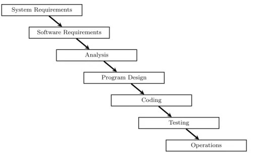
Figure 2.2 – The seven phases of the waterfall model, as described by Royce.

by MIT professor Jay Forrester for testing new ideas about social systems. This property is essential as it is the only way by which one can approach some level of reliability, considering the extreme complexity of the involved processes.

The first methodology, or model for software development, and by exten-sion systems development, that is relevant in this context, is the waterfall model, proposed by Royce in 1970 [50]. In his seminal publication, Royce starts by conceptualising the process of software development as a process in two steps: First, analysis, and second, coding, as shown in Figure 2.1. He then proceeds in a top-down manner to break down this very simple conceptual process into a perfectly ordered sequence of seven phases, each dependent upon completion of the preceding one, as shown in Figure 2.2.

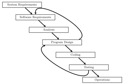
Modified versions of the waterfall model exist. Royce himself criticises his own proposal and improves his initial model with a “final model”, in which he adds feedback from code testing to design, and from design back to requirements, as shown in Figure 2.3. He also emphasises the importance of the following factors: involving the customer, testing, and documentation

throughout the entire process (figure 2.4). System Requirements Software Requirements Analysis Program Design Coding Testing Operations

Figure 2.3 – The phases of Royce’s final model, with the two critical back arrows.

Nowadays, it is argued that the model and its underlying philosophy of “big design up front”, while having undeniable advantages for some complex systems, like for instance its emphasis on documentation, is suitable only for projects which are stable, in other words projects that don’t have changing requirements. This is the case of equipment manufacturing for example, but the approach is not well adapted to the design and development of all modern software systems, where the requirements are very often not precise in the first place, and are subject to change.

Later on, confronted with the limits of the waterfall model for software development identified by Royce, people in the development trade tried to formulate a methodology that would better take into account the iterative nature of software or system development, and could accommodate both top-down [28] and bottom-up approaches, thus coping with the inevitable changes in requirements during a system’s life cycle. Iterative development means developing in phases, starting with a design goal, and ending with the client reviewing the progress. In the mid-eighties, Boehm published an article about the spiral model, not the first to discuss iterative development in this context, but the first after Royce to explain why iteration matters so

Figure 2.4 – The complete break-down of the Waterfall Model, as Royce himself described it in his 1970 publication [50] (figure 10).

Figure 2.5 – Hermes 2003, the Swiss project management method, which was the standard for the Swiss Administration until 2013, with its phases and decision points (in French). Note the similarities with the waterfall model in Figure 2.2.

much [7]. The spiral model was adopted by the US Military, for its ability to handle large, complex and critical systems in highly inflexible administrative environments.

It is interesting to note that many “modern” IT project management methods in the industry, in particular in corporate IT, are still very much inspired by Royce’s waterfall model, despite criticism. Hermes, the standard of the Swiss Federal Administration [61], for example, consists of a more or less iterative version of a waterfall in six phases, now reduced to model only four phases in its fifth version [60] (Figures 2.5 and 2.6). The tendency is to speak of “frameworks”, and not “methods” or “methodologies” any more. It is always difficult to see through the haze of buzz words in corporate IT, but this might indicate a decreasing trust in the gospel that such methods are applicable, even for managers.

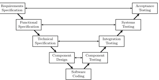
The V-Model, which is widespread in the German Administration, is no different in essence. It emphasizes testing, by relating each development phase to a validation equivalent on the other side of the V, as shown in Fig-ure 2.7. In the commercial world also, the Rational Unified Process (formerly Rational, now IBM), ends up to be very similar, at least with respect to our current considerations.

Figure 2.6 – hermes 5, the Swiss project management method, with its phases and decision points (in French). Note the trend to reduce the number of phases and provide for more flexible frameworks, exemplified with the differences between this figure and the previous version of hermes shown in Figure 2.5.

Requirements Specification Acceptance Testing Functional Specification Systems Testing Technical Specification Integration Testing Component Design Component Testing Software Coding

Figure 2.7 – One version of the V-Model. Note the linearity, despite the rela-tions between activities on the right branch with those on the left branch of the V.

models led to the chaos model, defined by Raccoon1 _{[45]. The idea is that all}

phases of the life cycle apply to all levels of a project, so a chaos strategy is devised that takes into account these properties, hence bridging the gap between managerial models (waterfall, spiral) and software development methodologies. For example, individual lines of code are treated as a level requiring design, implementation and integration, and so are functions, mod-ules, systems and finally the whole project. This fractal structure, inspired by chaos theory, despite its obvious cynicism, is arguably closer to how soft-ware is actually developed. Indeed, it shows that the development of any sufficiently complex system consists in many interrelated levels of problem solving. Any attempt to bridge the gap between management and develop-ment has to take these properties into account, or it is doomed to fail. This essential property of software development was already identified by Brooks in his book “The Mythical Man-Month” [9] and his paper “No Silver Bullet: Essence and Accidents of Software Engineering” [10], where he advocates that software is not built, but grown.

Also during the eighties, at IBM, James Martin developed a completely different approach called rapid application development (RAD), that he formalised in a book in 1991 [26]. The focus is on delivering quality as fast as possible. The speed is achieved through the use of Computer Aided Software Engineering (CASE) tools, and the quality through the early involvement of users in the analysis and design phases. The approach enables an early proto-type delivery, with reduced features, usually, and the subsequent incremental addition of more features.

Rapid Application Development consists in six core elements:

1. Prototyping: developing a feature-light application in a very short amount of time.

2. Iterative development: adding features in short life cycles, feeding the new user requirements into the next release.

3. Time boxing: supporting iterative development by pushing off fea-tures to future versions.

4. Team members: emphasizes that teams should be small and com-posed of experienced members.

5. Management approach: management should be very involved in keeping life cycles short and enforcing deadlines.

6. RAD tools: development speed is more important than the cost of tools, so one should use the latest technologies.

The major drawback of this approach is the reduced scalability of the result-ing systems, a consequence of the continuous enhancement of an early imper-fect prototype. This requires heavy re-factoring, continuous non-regression testing and the system quickly becomes impossible to maintain. Also, it has limited value as such for this context, as it is almost entirely unstructured.

During the nineties, moving further away from the plan-driven and pre-dictive waterfall model towards more adaptive methods, a variety of methods have been defined and grouped under the general framework denomination of agile software development, since 2001 [5]. The basic idea was to further re-fine iterative methods by dramatically reducing the time between releases, or milestones, now measured in weeks or even days instead of months. Another common denominator of these methods is that work is performed in a highly collaborative manner, with many concurrent activities and synchronisation of dependencies.

The well-known agile software development methods include extreme programming [4], Scrum [56], agile modelling, adaptive software develop-ment [19], Crystal methodologies, dynamic systems developdevelop-ment method [14], feature driven development [34], lean software development [40], agile unified process, most of which are arguably modern corporate IT consultant hypes. Nevertheless, interesting for our case, as they involve well defined roles and processes.

It is worth mentioning that the same “agile” approach has been applied to the documentation and data life cycles, as was the case for Royce forty years ago.

2.1.2

Towards Formalisation

Regardless of the criticism of the methods mentioned in the previous section, it is not unusual to find one method used within another on some scale or other. Indeed, an essential property of all these models is that they define some common phases or activities, thus forming building blocks, at different levels of granularity.

For example, a developer might use the waterfall model on a very small scale for the development of his module, while an agile software development method is applied by the team for the whole project. The reverse is also highly probable, in particular where financial constraints impose a waterfall management of the project with decision points, whereas the developers work with agile methodologies, and short release cycles. So not only are

Initiation

System Concept Development Planning

Requirement Analysis Design

Development

Integration and Test Implementation

Operation and Maintenance Disposition

Figure 2.8 – The ten steps of the SDLC as proposed by the Department of Justice.

methodologies applicable at all levels of software development, as stated in the chaos model, they are also intertwined and combined. This shows the need for a clear definition of common subprocesses, or building blocks, in all approaches, that could be formalised and combined to create any new method, customised for the specific needs of the project managers or entire teams.

A first step in this direction has been taken by big administrations, not-ably by the US Department of Justice, who defined the Systems Development Life Cycle (SDLC) [59]. The involved systems approach to problem solving, made up of several phases, in this case ten, is shown in Figure 2.8.

The systems development life cycle also includes documentation as de-liverables that must be generated during each phase. The same approach is used in hermes, the Swiss IT project management method (or framework), with a linear process similar to the waterfall model, and emphasis on doc-umentation and decision points [61, 60]. Figure 2.6 shows the phases of the method and its decision points. Note that hermes is meant to be tailored, so by default no documentation is mandatory, apart from the description of the projet itself and its organisation (the project manual).

Although it is an essential step towards a more formal methodology, it is intended to be read, interpreted, validated and applied by human beings.

In order to have a system able to represent and validate such models auto-matically or semi-autoauto-matically, which is the ultimate goal of this research, a good formalisation with appropriate state of the art knowledge repres-entation techniques is necessary, something that couldn’t be found in this domain, at least not explicitly.

Following today’s call for standards and best practices in software and systems development, the International Organization for Standardization (ISO) and the International Electrotechnical Commission (IEC) established a joint technical committee in 1987 with the scope of standardization in the field of information technology systems. This committee initiated the development of an International Standard, ISO/IEC 12207 for software life cycles [22], that led to its IEEE/EIA industry implementation in 1998 [21]. The standard establishes a top-level software life cycle architecture. The life cycle begins with an idea, or a need, that can be satisfied wholly or partly by software, and ends with the retirement of the software, as in the SDLC or hermes. The architecture is built with a set of processes and interrelation-ships among them. The processes are modular, minimally coupled, and the strict responsibility of a party, or role, in the software life cycle. That means that processes are as independant from each other as possible, and reused as building blocks where possible, and that to each activity or process, a role can be assigned.

This standard is meant for specific projects, typically led by project man-agers using check lists for the validation of the various phases, also a core activity of hermes for instance. It is, however, the closest thing to a formal definition to be found to this day for this specific context, so it was chosen as the starting point for the practical validation of our approach (Chapter 4).

2.2

Finite State Automata

The theory of finite state automata (FSA), or finite state machines (FSM), is a well-established model, used mainly for the representation of linear be-havioural processes, as in computer programs. This section gives the basic definitions of finite state automata, as it relates to our context. More formal details, exhaustive classifications of various FSA, and their properties, are extensively described in the appropriate literature [17, 18, 11].

A finite state automaton consists in a finite set of states, and a finite set of transitions. The latter indicates a change of the machine from one state to another, and is triggered by a certain condition or event. An auto-maton can only be in one state at a time, and only one transition can be activated at a time (determinism). Non-deterministic finite state automata

S0 S Sn

δ1 δ2

Figure 2.9 – A traditional graphical representation of a finite state automaton with three states S = {S0, S, Sn} and two transitions ∆ = {δ1, δ2}. S0 is the

only initial (or start) state, S is the single intermediate state, and Sn is the

only final (or end, or accepting) state.

(NFA) also exist, but these are irrelevant in practical settings, such as the context of this thesis. It has been demonstrated that any non-deterministic finite state automaton can be transofrmed into a deterministic one through an algorithm: the Rabin and Scott powerset construction algorithm [44]. definition. A finite state automaton over an alphabet Σ is a quintuple

A=_{{Σ, S, ∆, I, F }, where}

• S is a finite set of states, with S 6= ∅; • ∆ : S × Σ → S is a finite set of transitions; • I ⊆ S is the set of initial states, with I 6= ∅;

• F ⊆ S is the set of final states, which can be empty.

Graphically, finite state automata are represented using circles and ar-rows. Initial (or start) states are represented with a dashed line, intermediate events as solid circles, and final states with a thick line, or a double line. This is the notation that was chosen in the remainder of this document. Trans-itions are simple arrows, sometimes with a label. Figure 2.9 shows a simple state machine with three states and two transitions as an illustration of the notation.

2.3

Business Process Model and Notation

Business process model and notation (BPMN), previously known as “Busi-ness process modelling notation”, is a graphical representation of process work flows, and a widely accepted standard to model any business activities in the managerial world. It was initially developed by the Business Process Management Initiative, and has been maintained by the Open Management Group since 2005 [58].

BPMN consists in a minimal set of graphical elements, used to construct diagrams called Business Process Diagrams (BPD). There are four categor-ies of elements: flow objects, connecting objects, swim lanes, and artefacts.

These elements are described below, and a summary with the matching graphical representations is provided in Table 2.1 (page 22).

1. Flow objects: Events, activities, gateways

2. Connecting objects: Sequence flow, message flow, association 3. Swim lanes: Pool, lane

4. Artefacts: Data object, group, annotation

Events. An event denotes something that happens (compared to

some-thing that is done = an activity). It is represented with a circle (table 2.1), and can contain icons denoting the type of event (e.g., an envelope for a message, or a lightning bolt for an error). Events can be “catching”, in which case they receive something (typically a message) and start a process, or “throwing”, in which case they send something (typically a message) when a process ends. There are three types of events, similar in representation to the common notation of finite state machines (section 2.2): start, intermediate and end events.

Start events. A start event is a trigger for a process. The consequence is that it can only be the “catching” type.

Intermediate events. An intermediate event represents what is hap-pening between start and end events. Therefore, it can be “catching” or “throwing”.

End events. An end event represents the end of a process. It can only be the “throwing” type. For instance, it can launch another process by sending a message to a catching event.

Activities. An activity represents the actual work being done. It is similar

to the label on a transition in a finite state machine. It’s graphical represent-ation is a rectangle with rounded corners, with a label inside. The rectangle’s line differs, depending on the the type of activity and may contain an icon. There are four types of activities: tasks, sub processes, transactions, and call activities.

Tasks. A task represents an atomic unit of work. The criterion for atom-icity is that it cannot be broken down to a further level of detail.

Sub processes. A sub process is the mean to provide a zooming feature in a diagram. The idea is to hide/reveal additional levels of detail by collapsing/revealing the more detailed process when clicking the plus sign in the activity. A sub process must have a start event, and one or several end events, and the flows from the parent process must not cross its boundary.

Transactions. A transaction is a special kind of sub process where all contained activities must be treated as a whole. It is similar to transac-tions in the context of persistence (databases): all activities must all be completed to proceed further, and if any one of these fails, they must all be undone (roll-back). The graphical representation is a double border surrounding the sub process.

Call activities. A call activity is a point where a global process (or task) is reused. It provides the ability to reuse elements, combine them, and is an essential feature of process work flow modelling, like the sub process. The graphical representation is a thick border around the rect-angle.

The sub process and call activities are very interesting features, as they provide composition and synchronisation mechanisms, which is essential to the systems thinking approach to problem solving which constitutes a leit-motiv of this research, and is the core idea behind the first contribution presented in Chapter 3.

Gateways. A gateway is a point of forking or merging of process paths.

Its representation is a diamond shape, with an icon inside denoting the type of condition. This is similar to older popular work flow notations. There are seven different types of conditions, hence seven gateways: exclusive, event based, parallel, inclusive, exclusive event based, complex, and parallel event based.

Exclusive. The exclusive gateway provides an alternative. Only one of the paths can be taken as in an exclusive or (XOR).

Event based. The event based gateway provides a condition based on the evaluation of an event to determine the path to be taken.

Parallel. The parallel gateway provides a branching point for parallel paths without condition.

Inclusive. The inclusive gateway provides alternative flows, where all paths are evaluated.

Exclusive event based. An exclusive event based gateway is simply the combination of exclusive and event based gateways described above. The condition is the event being evaluated and the path to be taken is de-termined based on this. The paths are mutually exclusive.

Complex. A complex gateway can be used to model a complex syn-chronization mechanism. For example, a mechanism where more than

two choices depend on ranges of values (if0 < x_{≤ 5 then choose path 1,}

else if 5 < x≤ 10 then choose path 2, else if ... then choose path n − 1,

else choose path n).

Parallel event based. The parallel event based gateway is the combin-ation of the parallel and the event based gateways. Parallel processes are started based on an event, but since the parallel gateway works without condition, there is no evaluation of the event.

Connecting objects. Connecting objects, or connections, are used to

con-nect flow objects (events, activities, gateways) with each other. They are of three types: sequences, messages, and associations.

Sequence flows. A sequence flow simply shows the order in which activ-ities are performed. Its representation is a solid line and an arrowhead. The sequence flow may be specialised: to indicate one of several condi-tional flows from an activity, a diamond is added at the start of the arrow. Another special case is to denote the default flow from a decision (or activity) with conditional flows, in which case a slash (small diagonal line) is prepended to the arrow.

Message flows. A message flow is used to represent the passing of mes-sages across boundaries (pools, see below). Its representation is a dashed or dotted line, an open circle at the start (sometimes a diamond, in which case it is not to be confused with the continuous line of the conditional sequence flow), and an empty arrowhead at its end. A message flow is to be used strictly across pools, and can never be used within the same pool.

Associations. An association is used to associate an artefact or text to a flow object. Its representation is a dotted line. An association can include a direction, in which case an arrowhead is added: toward the artefact to represent an output, from the artefact to represent an input, or both to indicate it is an input as well as an output.

Swim lanes. Swim lanes are a way to organize elements into categories. They are represented as rectangles with names, separated by solid lines. The only way to link elements from one swim lane to another is by message flow. Swim lanes are of two types: pools and lanes.

Pools. A pool groups the major participants of a process. Usually, it is used to separate different organisations. It is represented as a rectangle with a label. A pool can contain one or more lanes, like an actual swim-ming pool. Visually, a pool can be open, showing all internal details, or collapsed to hide the detail, in which case it is only a rectangle spanning the entire diagram.

Lanes. A lane groups activities inside a pool according to function or role. It is represented as a rectangle spanning the entire width of the pool (or height if the diagram is vertically arranged). A lane contains the flow objects, connecting objects and artefacts.

Artefacts. Artefacts are available to bring more information into the

dia-gram, thus rendering it more readable. There are three pre-defined artefacts: data objects, groups and annotations.

Data objects. Data objects show which data is required or produced in an activity. Its representation is a cornered sheet, like a document in many file systems explorers. It is often used for documentation artefacts. Groups. A group is a visual grouping of activities. It does not affect the flow in any way. Its representation is a rectangle, with rounded corners and dashed or dotted lines.

Annotations. An annotation does not affect the flow either, but it brings more information about flow objects, for example a comment. Its representation is a big left bracket spanning the entire text of the annotation.

A simple example of a BPMN diagram is depicted in Figure 2.10 on page 23. It is important to note, that BPMN permits the extension of the basic set presented here with other artefacts, if deemed necessary.

Category Elements Graphical notations Flow objects Events Activities Gateways Connecting objects Swim lanes Artefacts Table 2.1 – BPMN Elements

Figure 2.10 – An example of a BPMN diagram mo del: a simplified hotel chec k-in pro cess.

2.4

Petri Nets

Petri nets are a well-established formalism used for the modelling and ana-lysis of concurrent systems [35]. This section gives a basic definition of Petri nets and their relevant associated concepts: multisets, pre-/post-sets, mark-ing, firmark-ing, computation. More detailed or various definitions can be found in the extensive literature [35, 48, 49, 29, 63].

definition. A multiset, over a non-empty finite set S, is a mapping

defined as m: S _{→ N. The non-negative number m(s), where s ∈ S,}

repres-ents the number of occurrences of the element s in the multiset m. The set

of all the multisets over S is denoted by NS_.

definition. A Petri net is a tuple N = (P, T, F, W ), where

• P is a finite set of places and T is a finite set of transitions, such that

P _{∩ T = ∅;}

• F ⊆ (P × T ) ∪ (T × P ) is the flow relation;

• W : (P × T ) ∪ (T × P ) → N is the weight function for N, such that W(x,y) = 0 iff (x, y) /∈ F .

The Petri nets defined above are also known as place-transition Petri nets (or P/T Petri nets).

definition. If x∈ P ∪ T , then:

• The pre-set of x is the set: •x = {y|(y, x) ∈ F }; • The post-set of x is the set: x• = {y|(x, y) ∈ F } .

definition. A marking of a Petri net N = (P, T, F, W ) is a mapping

M : P _{→ N. It assigns a number of tokens to each place p ∈ P .}

definition. A marked Petri net is a pair µ = (N ; M ), where N is a Petri net and M is a marking of N .

definition. Let N = (P, T, F, W ) be a Petri net, M a marking of N and

t _{∈ T a transition from N:}

• t is enabled in marking M if W(p,t) ≤ M(p),∀p ∈ P ;

• If t is enabled in marking M, then t can fire, yielding a new marking

The firing rule can be extended to sequences of transitions:

definition. A computation, or maximal execution sequence, is a finite execution sequence which ends with a marking in which no transition is enabled, or an infinite execution sequence.

definition. A marking M0 is reachable in one step from another

mark-ing M if there exists a transition t_{∈ T such that M →}T M0. By extension to

a sequence of transitions, a marking M0 is reachable from another marking

M if there exists a transition sequence σ _{∈ T}∗ such that M _→∗_T M0, where

→∗

T denotes the reflexive transitive closure of the transition relation →T.

definition. The set of reachable markings R(µ) of a marked Petri net

µ from an initial marking M0 is the set of all reachable markings from M0:

R(µ) =_{M0

|M0 →∗T M

0

}

definition. The reachability graph, or state space, of a marked Petri

net µ is the transition relation_→T restricted to its reachable markings R(µ).

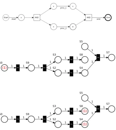
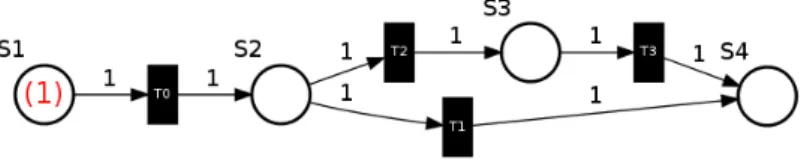
Graphically, a Petri net is represented as a graph of places and transitions. Places are represented as circles, and transitions as rectangles with inbound and outbound arrows. Both are labelled. The inbound, and outbound arrows show the number of tokens that are respectively consumed, and produced by the transition. Tokens in places are usually represented by small circles or bullets, or by a number in brackets or parenthesis.

Figure 2.11 shows the graphical representation which was chosen for the remainder of this document, and which is also what is being generated by the prototype described in Appendix A.

Formally the Petri net N in Figure 2.11 is defined as :

N = (P, T, F, W ) where P =_{{S1, S2, S3, S4}} T ={T 0, T 1, T 2, T 3} F =_{{(S1, T 0), (T 0, S2), (S2, T 1), (T 1, S4),} (S2, T 2), (T 2, S3), (S3, T 3), (T 3, S4)_}

The weight function W assigns 1 to a couple (Si, T j) iff (Si, T j) _{∈ F ,}

The initial state, with a single token in S1. The marking is M0= {S1 = 1, S2 = 0, S3 = 0, S4 = 0}. Only transition T0 is enabled.

After transition T0 has fired, the token is in S2. The marking is M0= {S1 = 0, S2 = 1, S3 = 0, S4 = 0}. Both transitions T1 and T2 are enabled.

First possibility: after transition T1 has fired, the token is in place S4. The marking is M0= {S1 = 0, S2 = 0, S3 = 0, S4 = 1}. No transition is enabled, the maximal execution

sequence has been reached, so the computation ends.

Second possibility: After transition T2 has fired, the token is in place S3. The marking is M0= {S1 = 0, S2 = 0, S3 = 1, S4 = 0}. Transition T3 is enabled.

After transition T3 has fired, the token is in place S4. The marking is

M0= {S1 = 0, S2 = 0, S3 = 0, S4 = 1}. No transition is enabled, the maximal execution sequence has been reached, so the computation ends.

Figure 2.11 – An example of a graphical representation of a simple Petri net, in its successive possible states depending on which transition fires.

2.5

Social Protocols

Social protocols were proposed in 2006 by Willy Picard as a model for ad-aptive human collaboration processes [36]. They are presented in this section as they formed the starting point for our research.

The social protocols provide a formalism to model interactions between humans. The formal definition of a social protocol, given in Picard’s public-ation [36], can be summarised as the following abstract concepts, presented in a bottom-up approach:

definition. An action a is the execution of a task. definition. A role r is a label.

definition. A behavioural unit is a group BU = R× A. For example:

“The manager writes the final report” is a behavioural unit where the role is “manager” and the action is ”write the final report”.

definition. A state s is a label associated with a given situation in a collaborative process.

definition. A transition is the combination of a starting (source)

state and an ending (destination) state with a behavioral unit: t =

(bu, ssource, sdestination).

Once these preliminary definitions are in place, one can define a social pro-tocol as the set of all states and transitions.

Picard adds a desirability function∆, adding external constraints on the

execution of the behavioural units, thus specifying the probability that the transition will be activated. The social protocol is then defined as:

definition. A social protocol is a sextuple

Σ ={S, Sstart

, Send, R, A,∆}

where

• S is the set of all states s.

• Sstart _{is the set of starting (source) states s}

source, with Sstart ⊂ S.

• Send _{is the set of end (destination) states s}

destination, with Send⊂ S

• R is the set of roles r. • A is the set of actions a.

• ∆ : T → [0, 1] is the set of desirability functions associated with the behavioural units formed by the elements of R and A.

This forms a (non-deterministic) finite state automaton as described in Sec-tion 2.2, with the addiSec-tion of some external constraint on the choice of trans-itions provided by the desirability function.

The interpretation of a social protocol is that the process is moving from state to state via the execution of behavioural units. But one has to be careful that a behavioural unit may only be executed by a collaborator labelled with the appropriate role.

This last property is very interesting as it allows for the modelling of SDLC processes as described in documents such as the DoD definition of SDLC [59], the IEC/IEEE 12207 document [22] or hermes [61, 60], already discussed in Section 2.1.2.

The desirability function is an interesting idea, as it allows for the mod-elling, for example, that the transitions leading to success are more desirable than the transitions leading to failure. Moreover, it provides a mechanism to model negotiation.

Negotiation consists in changing the desirability function, or even chan-ging the structure of a model. This is deemed necessary because human sys-tems are constantly changing and adapting. For instance, with experience, actors in a process can observe that a new transition is needed, or that some transitions are all of a sudden, less “desirable” than others.

It is interesting to note at this point that the desirability function as such disappeared from the model in subsequent publications by the same author [37, 38, 39]. It influenced our initial approach in a very significant manner; in fact, it was the main reason why we chose Picard’s social protocols in the first place, although it became irrelevant in the course of our research as well, as we focused on providing a representation that is as simple as possible, and the potential tailoring of processes is outside the scope of the model itself. It could nevertheless be an important research path to pursue, in relation to our context, as it is an essential feature of human activity, as Picard states [36].

The Model

This chapter presents the first step of this thesis’ contribution, i.e. the model to represent SDLC processes. Although it was inspired initially by the social protocols presented in Chapter 2, it consists merely in a finite state machine (FSM), to which two extensions are made to represent parallel synchronised sub-processes on the one hand, and allow for scalability on the other hand. The first section presents the argument that led from Picard’s idea to this very simple model. The subsequent two sections explain the two necessary extensions, followed by a formal definition of the model, with the necessary definitions. The last section presents the mapping of the model to Petri nets.

3.1

Argument

As already stated in the introduction, when it comes to dealing with pro-cesses, there is a clear gap between the management world and formalism. The essence of this gap lies in the different points of view and the needs of each of these worlds.

Management is concerned with processes in terms of people, results, and possibly representation as a means to communicate ideas. There is usually no need to scientifically prove the models, as common agreement usually suffices. In management, BPMN is one de facto process modelling standard. These models are agreed on, stored for later use or used as ERP workflows or other management systems.

On the other hand, formalisations provide these proofs. The mathematic-ally sound representations, such as Petri nets or finite state automata, allow many interesting analysis or validation of properties at the formal level. They provide both a good and compact graphical representation, but if one was to attempt to model processes such as those in the DoJ SDLC document, the

IEC/IEEE 12207 document [22], or even hermes 5, it would be impossible to ensure that the model really copes with reality, as it quickly become far too complex to be tractable.

One reason for this is the difficulty for people in general, and people in the management world in particular, to apply systems thinking to the formalisations with theoretical models such as finite state automata or Petri nets, like they would with BPMN if they were well-trained business analysts for example. Indeed, BPMN provides the mechanism for composing processes with sub-processes which facilitates the breaking down of the problem into sub-problems: the sub-process activity flow object (table 2.1 on page 22).

Finite state automata and Petri nets lack this composition (or zoom-ing) mechanism. Nothing prevents people from breaking down problems into models using those formalisms. This is actually what experienced people in-volved in modelling would do. But the representation do not encourage such methodologies, and we argue that this is a serious limitation for this par-ticular context. Recursive finite state machines [3] do provide it, and even in a very elegant generalised way. But they are very difficult to use in this context, due to the strict definitions permitting recursion, which in turn is not necessarily the way people think, unless they have been trained as mathematicians or computer scientists.

The same lack of simplicity de facto rules out the concepts of abstraction and folding in Petri nets [16] as well.

Moreover, the very nature of systems life cycle management processes, or any business process for that matter, implies the possibility to have parallel, concurrent activities. BPMN allows this, with swim lanes and coordination mechanisms through messages (table 2.1 on page 22). Petri nets too, as they were designed exactly for such problem, but they are still quite complex, and not commonly seen in the management world. Finite state automata simply lack this property, so they are not applicable.

The first step in starting to bridge the gap was to come up with a simple enough model that could represent processes with both the necessary prop-erties of composition and of concurrency, while retaining at least some math-ematical properties to allow for the validation of the properties of the work flow at a graphical or algorithmic level. Social protocols (section 2.5) seemed to be a very promising idea, as they were based on mathematical foundations, in this case finite state automata theory, and they were aimed at modelling and even negotiating processes. They suffer from the same limits as the fi-nite state automata in general, i.e. the lack of composition and concurrency mechanisms.

pro-posing to model his social protocols with coloured Petri nets [23]. This is described in details in “Modelling Multithreaded Social Protocols with Col-oured Petri Nets” [38]. The purpose of the development of social protocols is to model human-to-human interactions over a network from the ground up, while retaining a strong mathematical foundation, and explore the pos-sibilities offered by successive refinements of the model, for example a direct structural validation [37] or the application to agile paradigms of software development [39].

The use of coloured Petri nets in this context implies that the semantics of what is being produced is attached to the states themselves. Adding types would permit the explicit representation of what is being produced, a specific document or a software module for example, but this information would have to be explicit in the simple representation of the processes, and that would add complexity and burden to the users, by making the proposed model more complicated [52, 53]. This possible approach was therefore not investigated in our research, not because it was not interesting or not applicable, but because it was too anchored in the formalism world and not exactly aligned with our line of research, and it seemed more promising to attempt to bridge the gap between the two worlds with a simpler and more pragmatic proposal. After all, if one is to attempt to bridge the gap between two very differ-ent cultures, as is the case here, it would be a mistake to try to force the aspects of one culture on the other, and hope that by convincing managers that they should behave like scientists, their problems would be solved. To have better chances of success, it is better to try to retain as much of the characteristics of the two cultures, and connect these somehow. In this case, this means retaining the pragmatism of the managerial world on one side, and the formalism of the technical world on the other.

This led to the first idea, that was to retain the simplicity of finite state automata theory as it was applied in Picard’s first model of social proto-cols, i.e. with actions and roles, and extend it with only the two necessary properties to model composition, and concurrency. This is the essence of the model presented in this chapter: component state machines (CSM) and scal-able state machines (SSM), which together provide a simpler representation than BPMN, with less elements, but with a substratum of mathematical properties, that we will argue in Section 3.5 is not lost by the addition of the extensions [51], and therefore allows a mapping to Petri nets, which in turn permits interesting validation of properties that the model itself doesn’t allow.

Petri nets are not the only theory with sufficient mathematical sound-ness to allow analysis and validation of properties. Other representational

possibilities for our model were investigated, namely: conceptual graphs [55] and description logic. The two theories possess sound mathematical found-ations, and are expressive languages, but this very last feature is what rules them out. Representing processes using conceptual graphs or description lo-gic (or any other first-order predicate lolo-gic for that matter), adds to the burden of representing dynamic activities explicitly, while Petri nets were designed from the ground up to fulfil that requirement. In addition, Petri nets have a very pragmatic graphical representation that fully reflects their formal foundations.

The theory of µ-calculus, on the other hand, is applied to model checking for systems [24], in particular those non-deterministic systems operating in “critical contexts” [15]. The modal logic of µ-calculus is even more complic-ated than first-order predicate logic though, so it rules out this approach too, although it would be interesting to investigate its differences and potential advantages over Petri nets for validation.

It would nevertheless be interesting to investigate more complex formal-isms, like coloured Petri nets, if only to verify our assumptions about sim-plicity as a means of bridging the gap between the two cultures.

3.2

Synchronisation

To model development processes in the context of SDLC, an essential feature to include is some sort of synchronisation mechanism between several paral-lel, or concurrent, sub-processes or activities. Finite state automata theory doesn’t include such possibilities: there is no AND on the nodes, only ORs (alternatives).

The first extension is a simple “rendezvous” type of synchronisation mech-anism to model parallel activities and hold subsequent dependant activities until all pre-requisites are completed.

Note that it is different from the “rendezvous” as it is defined in the con-text of parallelism. The latter synchronises threads (processes) that continue after having met at that point. In our case the parallel processes themselves do not continue, it is the whole process that is held until the parallel processes all reach a final state.

Graphically, the synchronisation is represented by an AND in a rectangle between the set of final states of the synchronised automata on the one hand, and the set of source states of the dependent activities on the other hand.

It is very important at this point to realise that the extension is not formally part of the mathematical model itself, but only a convenient way to represent concurrent activities using finite state automata. There is no such

Figure 3.1 – Synchronisation between two parallel automata: The AND on the left means that both red and blue state machines are started after S1. The AND on the right means that both final states of the red and blue state machines must be reached in order to proceed to the final state S7 of the whole process. The dashed arrows emphasise the fact that those arcs are not part of the model.

Figure 3.2 – Representation of an alternative (an OR) in finite state automata theory. The alternative is already part of the model, as only one outbound path can be chosen at any given state, in this case either the red or the blue one.

thing as an AND in finite state automata theory. The arrows are therefore dashed, to emphasise the fact that the arcs are not transitions of the state machine, and do not carry meaning about a role or an action.

Figure 3.1 shows an example of such a synchronisation, and the chosen notation, consistent with the traditional notation for finite state automata described in Section 2.2. In this particular example, a whole automaton is composed of states S1 to S7, and can itself be subdivided into two compon-ents: the red and blue automata respectively. The synchronisation is two-fold: first S2 and S3 are triggered by an AND with two outbound arrows, and second S4 and S6 must both be reached in order to proceed to the fi-nal state S7. The red and blue state machines are therefore parallel activities that can be conducted separately, but must both be finished before the whole process can continue.

An arbitrary number of sub-processes n >1 can be synchronised in this

manner.

Note that there is no need for an OR (XOR), as an alternative is already part of the state machine theory: a state with multiple outbound arcs rep-resents such an alternative, dependant on the conditions expressed by the arcs, as in Figure 3.2.

It could be argued that non-deterministic FSA already include the AND, as they allow for zero to n transitions from a given state by definition, but

we find this representation to be simpler to use and to map to Petri nets, as one clearly sees, graphically, the difference between an AND and an OR (XOR), which is not the case in non-deterministic FSA.

3.3

Components

If one sets aside recursive state machines [3], finite state automata theory doesn’t provide any clear decomposition and composition mechanisms allow-ing for the design of sub-processes separately and their subsequent combin-ation into more complex processes. This mechanism is an essential feature of process modelling though, as it allows a systemic approach to problem solving, which is the only way to have a chance to cope with the sheer com-plexity of the processes involved in this context. So this feature has to be added, but in the simplest possible way: by allowing the replacement of an arc by another finite state automaton representing the corresponding sub-process.

This extension can be seen as a sort of recursive definition, similar in es-sence to that of recursive state machines [3], which allows for the replacement of activities (arcs) in an FSM by another FSM. In other words, it allows the viewing of an activity as a simple transition, or as a more detailed process.

It was found to be much simpler than the definition of a recursive state machine though. It is based only on the semantic equivalence of two differ-ent state machines seen at differdiffer-ent levels of detail. In this sense it is more appropriate to speak of “zooming” or “scalability”, so we use the terminology “scalable state machine” (SSM) and “component state machine” (CSM) in the remainder of this document when we refer to the extended FSM used in our model.

Intuitively, as a prelude to a more formal definition of the model, there are two conditions to satisfy for this property to hold:

1. The source states (entry nodes), and the destination states (exit nodes), must be unequivocally identified and respectively identical for the con-sidered transition T and the finite state automaton representing the sub-process it represents. This corresponds to the requirement of a well-defined interface in the definition of a recursive state machine, with the limitation that we consider only one entry state and one exit state.

2. The role associated with an arc must be in phase with the “overall role” of the component automaton. A certain freedom exists as to how to define this “overall role”, depending on the semantics of the process.