HAL Id: hal-02328216
https://hal.archives-ouvertes.fr/hal-02328216
Submitted on 26 Jul 2020
HAL is a multi-disciplinary open access
archive for the deposit and dissemination of
sci-entific research documents, whether they are
pub-lished or not. The documents may come from
teaching and research institutions in France or
abroad, or from public or private research centers.
L’archive ouverte pluridisciplinaire HAL, est
destinée au dépôt et à la diffusion de documents
scientifiques de niveau recherche, publiés ou non,
émanant des établissements d’enseignement et de
recherche français ou étrangers, des laboratoires
publics ou privés.
discrepancy
Yating Lin, Gilles Ramstein, Haibin Wu, Raj Rani, Pascale Braconnot, Masa
Kageyama, Qin Li, Yunli Luo, Ran Zhang, Zhengtang Guo
To cite this version:
Yating Lin, Gilles Ramstein, Haibin Wu, Raj Rani, Pascale Braconnot, et al.. Mid-Holocene
cli-mate change over China: model–data discrepancy. Clicli-mate of the Past, European Geosciences Union
(EGU), 2019, 15 (4), pp.1223-1249. �10.5194/cp-15-1223-2019�. �hal-02328216�
https://doi.org/10.5194/cp-15-1223-2019 © Author(s) 2019. This work is distributed under the Creative Commons Attribution 4.0 License.
Mid-Holocene climate change over China:
model–data discrepancy
Yating Lin1,2,4, Gilles Ramstein2, Haibin Wu1,3,4, Raj Rani2, Pascale Braconnot2, Masa Kageyama2, Qin Li1,3, Yunli Luo5, Ran Zhang6, and Zhengtang Guo1,3,4
1Key Laboratory of Cenozoic Geology and Environment, Institute of Geology and Geophysics,
Chinese Academy of Sciences, Beijing 100029, China
2Laboratoire des Sciences du Climat et de l’Environnement, LSCE/IPSL, CEA-CNRS-UVSQ, Université Paris-Saclay,
Gif-sur-Yvette 91191, France
3CAS Center for Excellence in Life and Paleoenvironment, Beijing 100044, China 4University of Chinese Academy of Sciences, Beijing 100049, China
5Institute of Botany, Chinese Academy of Sciences, Beijing 100093, China
6Institute of Atmospheric Physics, Chinese Academy of Sciences, Beijing 100029, China
Correspondence:Haibin Wu ([email protected]) Received: 26 October 2018 – Discussion started: 13 November 2018 Revised: 27 May 2019 – Accepted: 4 June 2019 – Published: 2 July 2019
Abstract.The mid-Holocene period (MH) has long been an ideal target for the validation of general circulation model (GCM) results against reconstructions gathered in global datasets. These studies aim to test GCM sensitivity, mainly to seasonal changes induced by the orbital parameters (lon-gitude of the perihelion). Despite widespread agreement be-tween model results and data on the MH climate, some im-portant differences still exist. There is no consensus on the continental size (the area of the temperature anomaly) of the MH thermal climate response, which makes regional quan-titative reconstruction critical to obtain a comprehensive un-derstanding of the MH climate patterns. Here, we compare the annual and seasonal outputs from the most recent Paleo-climate Modelling Intercomparison Project Phase 3 (PMIP3) models with an updated synthesis of climate reconstruction over China, including, for the first time, a seasonal cycle of temperature and precipitation. Our results indicate that the main discrepancies between model and data for the MH cli-mate are the annual and winter mean temperature. A warmer-than-present climate condition is derived from pollen data for both annual mean temperature ( ∼ 0.7 K on average) and winter mean temperature (∼ 1 K on average), while most of the models provide both colder-than-present annual and win-ter mean temperature and a relatively warmer summer, show-ing a linear response driven by the seasonal forcshow-ing. By
con-ducting simulations in BIOME4 and CESM, we show that surface processes are the key factors creating the uncertain-ties between models and data. These results pinpoint the cru-cial importance of including the non-linear responses of the surface water and energy balance to vegetation changes.
1 Introduction
Much attention from paleoclimate studies has been focused on the current interglacial (the Holocene), especially the mid-Holocene (MH; 6 ± 0.5 ka). The major difference in the ex-perimental configuration between the MH and pre-industrial (PI) arises from the orbital parameters, which brings about an increase in the amplitude of the seasonal cycle of insola-tion in the Northern Hemisphere and a decrease in the South-ern Hemisphere (Berger, 1978). Thus, the MH provides an excellent case study on which to base an evaluation of the climate response to changes in the distribution of insolation. Great efforts have been devoted by the modelling community to designing MH common experiments using similar bound-ary conditions (Joussaume and Taylor, 1995; Harrison et al., 2002; Braconnot et al., 2007a, b). In addition, much work has been done to reconstruct the paleoclimate change based on different proxies at the global and continental scale (Guiot et
al., 1993; Kohfeld and Harrison, 2000; Prentice et al., 2000; Bartlein et al., 2011). The greatest progress in understand-ing MH climate change and variability has consistently been made by comparing large-scale analyses of data with simu-lations from global climate models (Joussaume et al., 1999; Liu et al., 2004; Harrison et al., 2014).
However, the source of discrepancies between model re-sults and data is still an open and stimulating question. Two types of inconsistencies have been identified: (1) the model and data showing opposite signs; for instance, pale-oclimate evidence from data records indicates an increase of about 0.5 K in global annual mean temperature during the MH compared with PI (Shakun et al.. 2012; Marcott et al., 2013), while there is a cooling trend in model sim-ulations (Liu et al., 2014). (2) The same trend being dis-played by both model and data but with different magni-tudes. Previous studies have shown that while climate mod-els can successfully reproduce the direction and large-scale patterns of past climate changes, they tend to consistently underestimate the magnitude of change in the monsoons of the Northern Hemisphere as well as the amount of MH pre-cipitation over northern Africa (Braconnot et al., 2012; Har-rison et al., 2015). Moreover, significant spatial variability has been noted in both observations and simulations (Pey-ron et al., 2000; Davis et al., 2003; Braconnot et al., 2007a; Wu et al., 2007; Bartlein et al., 2011). For instance, Mar-cott et al. (2013) reconstructed a cooling trend of global tem-perature during the Holocene, mainly from marine records (∼ 80 %). Based on 642 sub-fossil pollen data points, Mar-sicek et al. (2018) show that long-term warming defined the Holocene until around 2000 years ago for the European and North American continents. The different trends of pollen-and marine-based reconstructions indicate the spatial vari-ability of annual temperature change during the MH over the globe, which has already been investigated by Bartlein et al. (2010). That makes regional quantitative reconstruction (Davis et al., 2003; Mauri et al., 2015) essential to obtain a comprehensive understanding of the MH climate patterns and to act as a benchmark to evaluate climate models (Fis-cher and Jungclaus, 2011; Harrison et al., 2014).
China offers two advantages with respect to these issues. The sheer expanse of the country means that the continen-tal response to insolation changes over a large region can be investigated. Moreover, the quantitative reconstruction of seasonal climate changes during the MH, based on the new pollen dataset, provides a unique opportunity to compare the seasonal cycles for models and data. Previous studies in-dicate that warmer- and wetter-than-present conditions pre-vailed over China during the MH and that the magnitude of the annual temperature increases varied from 2.4 to 5.8 K spatially, with an annual precipitation increase in the range of 34–267 mm (e.g. Sun et al., 1996; Jiang et al., 2010; Lu et al., 2012; Chen et al., 2015). However, Jiang et al. (2012) clearly show a mismatch between multi-proxy reconstruc-tions and model simulareconstruc-tions. In terms of climate anomalies
(MH–PI), besides the ∼ 1 K increase in summer temperature, 35 out of 36 Paleoclimate Modelling Intercomparison Project (PMIP) models reproduce annual (∼ 0.4 K) and winter tem-peratures (∼ 1.4 K) that are colder than the baseline, and a drier-than-baseline climate in some western and middle re-gions over China is depicted in models (Jiang et al., 2013). Jiang et al. (2012) point out the model–data discrepancy over China during the MH, but the lack of seasonal reconstruc-tions in their study limits comparisons with simulareconstruc-tions.
An important issue raised by Liu et al. (2014) is that the discrepancy at the annual level could be due to incorrect re-constructions of the seasonal cycle, a key objective in our paper. Moreover, it has been suggested that the vegetation change can strengthen the temperature response at high lati-tudes (O’Ishi et al., 2009; Otto et al., 2009), as well as alter the hydrological conditions in the tropics (Z. Liu et al., 2007). However, compared to the substantial land cover changes in the MH derived from pollen datasets (Ni et al., 2010; Yu et al., 2000), the changes in vegetation have not yet been fully quantified and discussed in PMIP3 (Taylor et al., 2012).
In this study, we first present new reconstructions. We use a quantitative biomization method to reconstruct veg-etation types during the MH based on a new synthesis of pollen datasets and then use an inverse vegetation model (Guiot et al., 2000; Wu et al., 2007) to obtain the mean annual temperature, the mean temperature of the warmest month (MTWA), the mean temperature of the coldest month (MTCO), the mean annual precipitation, July precipitation and January precipitation over China for the MH. Fur-thermore, we present a comprehensive evaluation of the PMIP3 simulations performed with state-of-art climate mod-els based on our reconstructions of temperature and precip-itation. This is the first time that such progress towards a quantitative seasonal climate comparison for the MH over China has been made. This point is crucial because the MH PMIP3 experiment is essentially one that looks at the re-sponse of the models to changes in the seasonality of in-solation, and the attempt to derive reconstructions of both summer and winter climate to compare with the simulations will thus enable us to answer the question posed by Liu et al. (2014) on the importance of seasonal reconstructions.
2 Data and methodology
2.1 Data
In this study, we collected 159 pollen records covering most of China for the MH period (6000 ± 50014C yr BP) (Fig. 1). Notably, according to IntCal13 (Reimer et al., 2013), the MH time slice of 6000 ± 50014C yr BP is about 6800 cal BP (the average value), which is not totally consistent with the “mid-Holocene” used in the CMIP5–PMIP3 experiment (6000 cal BP). But for a better comparison with BIOME6000 (in which the MH is defined as 6000 ± 50014C yr BP), we decided to choose the pollen data at 6000 ± 50014C yr BP
Figure 1.Distribution of pollen sites during the mid-Holocene pe-riod in China. The black circle is the original China Quaternary Pollen Database, red circles are digitized ones from published pa-pers and green circles represent the three original pollen data points used in this study. The area in green represents the Tibetan Plateau, and yellow represents the Loess Plateau.
in our study. In the 159 records, 65 were from the China Quaternary Pollen Database (CQPD, 2000), 3 were origi-nal datasets obtained for our study and the others were dig-itized from pollen diagrams in published papers with a re-calculation of pollen percentages based on the total number of terrestrial pollen types. These digitized 91 pollen records were selected according to three criteria: (1) clearly readable pollen diagrams with a reliable chronology and a minimum of three independent age control points since the Last Glacial Maximum (LGM); (2) including the pollen taxa during the 6000 ± 50014C yr BP period with a minimum sampling res-olution of 1000 years per sample; and (3) abandoning the pollen records if the published paper mentions the influence of human activity. For the age control, different dating meth-ods are utilized in the collected pollen records, and we ap-plied CalPal 2007 (Weninger et al., 2007) to correct14C age into calendar age so that they can be contrasted with each other. For lacustrine records, if the specific carbon pool age is mentioned in the literature, the calendar age is corrected after deducting the carbon pool. Otherwise, the influence of the carbon pool is not considered. The age–depth model for the pollen records was estimated by linear interpolation between adjacent available dates or by regression. Using ranking schemes from the Cooperative Holocene Mapping Project, the quality of dating control for the mid-Holocene was assessed by assigning a rank from 1 to 7; 70 % of the records used in our study fell into the first and second classes (see Table 1 for detailed information) according to the Webb 1–7 standards (Webb III, 1985). Vegetation type was quan-titatively reconstructed using biomization (Prentice et al., 1996), following the classification of plant functional types (PFTs) and biome assignment in China by the Members of
the China Quaternary Pollen Database (CQPD, 2000), which has been widely tested in surface sediment. The new sites (91 digitized data points and 3 original data points) added to our database improved the spatial coverage of pollen records, especially in the northwest, the Tibetan Plateau, the Loess Plateau and southern regions, where the data in the previous databases are very limited.
Modern monthly mean climate variables investigated in this study, including temperature, precipitation and cloudi-ness (total cloud fraction), have been collected for each mod-ern pollen site based on the datasets (1951–2001) from 657 meteorological observation stations over China (China Cli-mate Bureau, China Ground Meteorological Record Monthly Report, 1951–2001). The MH soil properties and characteris-tics used in the inverse vegetation model were kept the same with PI conditions, which are derived from the digital world soil map produced by the Food and Agricultural Organiza-tion (FAO, 1995). The atmospheric CO2 concentration for
the MH was taken from ice core records (EPICA community members, 2004) and was set at 270 ppmv.
A three-layer back-propagation (BP) artificial neural net-work (ANN) technique was used for interpolation on each pollen site (Caudill and Butler, 1992). Five input variables (latitude, longitude, elevation, annual precipitation, annual temperature) and one output variable (biome scores) have been chosen in ANN for modern vegetation. The ANN has been calibrated on the training set, and its performance has been evaluated on the verification set (20 %, randomly ex-tracted from the total sets). After a series of training runs, the lowest verification error is obtained with five neurons in the hidden layer after 10 000 iterations. In our study, at each pollen site, we first applied the biomization method to get the biome scores for both the present day and the MH. The anomalies between past (6 ka) and modern vege-tation indices (biome scores) were then interpolated to the 0.2 × 0.2◦ grid resolution by applying the ANN. After that, the modern grid values were added to the values of the grid of paleo-anomalies to provide gridded paleo-biome indices. Finally, the biome with the highest index was attributed to each grid point. This ANN method is more efficient than many other techniques on the condition that the results are validated by independent datasets, and therefore it has been widely applied in paleoclimatology (Guiot et al., 1996; Pey-ron et al., 1998). The schematic diagram of ANN (Fig. S1) can be found in the Supplement.
2.2 Climate models
PMIP, a long-standing initiative, is a climate model evalua-tion project which provides an efficient mechanism for using global climate models to simulate climate anomalies for past periods and to understand the role of climate feedbacks. In its third phase (PMIP3; Braconnot et al., 2011), the models were identical to those used in the Climate Modelling Intercomparison Project Phase 5 (CMIP5) experiments. The
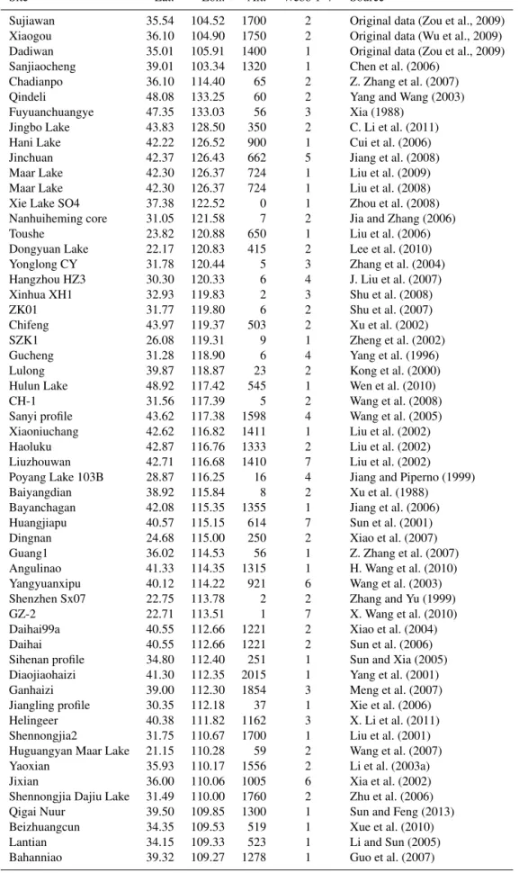
Table 1.Basic information on the pollen dataset used in this study.
Site Lat. Lon. Alt. Webb 1–7 Source
Sujiawan 35.54 104.52 1700 2 Original data (Zou et al., 2009) Xiaogou 36.10 104.90 1750 2 Original data (Wu et al., 2009) Dadiwan 35.01 105.91 1400 1 Original data (Zou et al., 2009) Sanjiaocheng 39.01 103.34 1320 1 Chen et al. (2006)
Chadianpo 36.10 114.40 65 2 Z. Zhang et al. (2007) Qindeli 48.08 133.25 60 2 Yang and Wang (2003) Fuyuanchuangye 47.35 133.03 56 3 Xia (1988)
Jingbo Lake 43.83 128.50 350 2 C. Li et al. (2011) Hani Lake 42.22 126.52 900 1 Cui et al. (2006) Jinchuan 42.37 126.43 662 5 Jiang et al. (2008) Maar Lake 42.30 126.37 724 1 Liu et al. (2009) Maar Lake 42.30 126.37 724 1 Liu et al. (2008) Xie Lake SO4 37.38 122.52 0 1 Zhou et al. (2008) Nanhuiheming core 31.05 121.58 7 2 Jia and Zhang (2006) Toushe 23.82 120.88 650 1 Liu et al. (2006) Dongyuan Lake 22.17 120.83 415 2 Lee et al. (2010) Yonglong CY 31.78 120.44 5 3 Zhang et al. (2004) Hangzhou HZ3 30.30 120.33 6 4 J. Liu et al. (2007) Xinhua XH1 32.93 119.83 2 3 Shu et al. (2008) ZK01 31.77 119.80 6 2 Shu et al. (2007) Chifeng 43.97 119.37 503 2 Xu et al. (2002) SZK1 26.08 119.31 9 1 Zheng et al. (2002) Gucheng 31.28 118.90 6 4 Yang et al. (1996) Lulong 39.87 118.87 23 2 Kong et al. (2000) Hulun Lake 48.92 117.42 545 1 Wen et al. (2010) CH-1 31.56 117.39 5 2 Wang et al. (2008) Sanyi profile 43.62 117.38 1598 4 Wang et al. (2005) Xiaoniuchang 42.62 116.82 1411 1 Liu et al. (2002) Haoluku 42.87 116.76 1333 2 Liu et al. (2002) Liuzhouwan 42.71 116.68 1410 7 Liu et al. (2002) Poyang Lake 103B 28.87 116.25 16 4 Jiang and Piperno (1999) Baiyangdian 38.92 115.84 8 2 Xu et al. (1988)
Bayanchagan 42.08 115.35 1355 1 Jiang et al. (2006) Huangjiapu 40.57 115.15 614 7 Sun et al. (2001) Dingnan 24.68 115.00 250 2 Xiao et al. (2007) Guang1 36.02 114.53 56 1 Z. Zhang et al. (2007) Angulinao 41.33 114.35 1315 1 H. Wang et al. (2010) Yangyuanxipu 40.12 114.22 921 6 Wang et al. (2003) Shenzhen Sx07 22.75 113.78 2 2 Zhang and Yu (1999) GZ-2 22.71 113.51 1 7 X. Wang et al. (2010) Daihai99a 40.55 112.66 1221 2 Xiao et al. (2004) Daihai 40.55 112.66 1221 2 Sun et al. (2006) Sihenan profile 34.80 112.40 251 1 Sun and Xia (2005) Diaojiaohaizi 41.30 112.35 2015 1 Yang et al. (2001) Ganhaizi 39.00 112.30 1854 3 Meng et al. (2007) Jiangling profile 30.35 112.18 37 1 Xie et al. (2006) Helingeer 40.38 111.82 1162 3 X. Li et al. (2011) Shennongjia2 31.75 110.67 1700 1 Liu et al. (2001) Huguangyan Maar Lake 21.15 110.28 59 2 Wang et al. (2007) Yaoxian 35.93 110.17 1556 2 Li et al. (2003a) Jixian 36.00 110.06 1005 6 Xia et al. (2002) Shennongjia Dajiu Lake 31.49 110.00 1760 2 Zhu et al. (2006) Qigai Nuur 39.50 109.85 1300 1 Sun and Feng (2013) Beizhuangcun 34.35 109.53 519 1 Xue et al. (2010) Lantian 34.15 109.33 523 1 Li and Sun (2005) Bahanniao 39.32 109.27 1278 1 Guo et al. (2007)
Table 1.Continued.
Site Lat. Lon. Alt. Webb 1–7 Source Midiwan 37.65 108.62 1400 1 Li et al. (2003b) Jinbian 37.50 108.33 1688 2 Cheng (2011) Xindian 34.38 107.80 608 1 Xue et al. (2010) Nanguanzhuang 34.43 107.75 702 1 Zhao et al. (2003) Xifeng 35.65 107.68 1400 3 Xu (2006) Jiyuan 37.13 107.40 1765 3 X. Li et al. (2011) Jiacunyuan 34.27 106.97 1497 2 Gong (2006) Dadiwan 35.01 105.91 1400 1 Zou et al. (2009) Maying 35.34 104.99 1800 1 Tang and An (2007) Huiningxiaogou 36.10 104.90 1750 2 Wu et al. (2009) Sujiawan 35.54 104.52 1700 2 Zou et al. (2009) QTH02 39.07 103.61 1302 1 Yu et al. (2009) Laotanfang 26.10 103.20 3579 2 W. Zhang et al. (2007) Hongshui River2 38.17 102.76 1511 1 Ma et al. (2003) Ruoergai 33.77 102.55 3480 1 Cai (2008) Hongyuan 32.78 102.52 3500 2 Wang et al. (2006) Dahaizi 27.50 102.33 3660 1 Li et al. (1988) Shayema Lake 28.58 102.22 2453 1 Tang and Shen (1996) Luanhaizi 37.59 101.35 3200 5 Herzschuh et al. (2006) Lugu Lake 27.68 100.80 2692 1 Zheng et al. (2014) Qinghai Lake 36.93 100.73 3200 2 Shen et al. (2004) Dalianhai 36.25 100.41 2850 3 Cheng et al. (2010) Erhai ES core 25.78 100.19 1974 1 Shen et al. (2006) Xianmachi profile 25.97 99.87 3820 7 Yang et al. (2004) TCK1 26.63 99.72 3898 1 Xiao et al. (2014) Yidun Lake 30.30 99.55 4470 4 Shen et al. (2006) Kuhai Lake 35.30 99.20 4150 1 Wischnewski et al. (2011) Koucha Lake 34.00 97.20 4540 2 Herzschuh et al. (2009) Hurleg 37.28 96.90 2817 2 Zhao et al. (2007) Basu 30.72 96.67 4450 3 Tang et al. (1998) Tuolekule 43.34 94.21 1890 1 An et al. (2011) Balikun 43.62 92.77 1575 1 Tao et al. (2010) Cuona 31.47 91.51 4515 3 Tang et al. (2009) Dongdaohaizi2 44.64 87.58 402 1 Li et al. (2001) Bositeng Lake 41.96 87.21 1050 1 Xu (1998) Cuoqin 31.00 85.00 4648 4 Luo (2008) Yili 43.86 81.97 928 2 X. Li et al. (2011) Bangong Lake 33.75 78.67 4241 1 Huang et al. (1996) Shengli 47.53 133.87 52 2 CQPD (2000) Qingdeli 48.05 133.17 52 1 CQPD (2000) Changbaishan 42.22 126.00 500 2 CQPD (2000) Liuhe 42.90 125.75 910 7 CQPD (2000) Shuangyang 43.27 125.75 215 1 CQPD (2000) Xiaonan 43.33 125.33 209 1 CQPD (2000) Tailai 46.40 123.43 146 5 CQPD (2000) Sheli 45.23 123.31 150 4 CQPD (2000) Tongtu 45.23 123.30 150 7 CQPD (2000) Yueyawan 37.98 120.71 5 1 CQPD (2000) Beiwangxu 37.75 120.61 6 1 CQPD (2000) East Tai Lake1 31.30 120.60 3 1 CQPD (2000) Suzhou 31.30 120.60 2 7 CQPD (2000) Sun Moon Lake 23.51 120.54 726 2 CQPD (2000) West Tai Lake 31.30 119.80 1 1 CQPD (2000) Changzhou 31.43 119.41 5 1 CQPD (2000) Dazeyin 39.50 119.17 50 7 CQPD (2000) Hailaer 49.17 119.00 760 2 CQPD (2000)
Table 1.Continued.
Site Lat. Lon. Alt. Webb 1–7 Source Cangumiao 39.97 118.60 70 1 CQPD (2000) Qianhuzhuang 40.00 118.58 80 6 CQPD (2000) Reshuitang 43.75 117.65 1200 1 CQPD (2000) Yangerzhuang 38.20 117.30 5 7 CQPD (2000) Mengcun 38.00 117.06 7 5 CQPD (2000) Hanjiang-CH2 23.48 116.80 5 2 CQPD (2000) Hanjiang-SH6 23.42 116.68 3 7 CQPD (2000) Hanjiang-SH5 23.45 116.67 8 2 CQPD (2000) Hulun Lake 48.90 116.50 650 1 CQPD (2000) Heitutang 40.38 113.74 1060 1 CQPD (2000) Zhujiang delta PK16 22.73 113.72 15 7 CQPD (2000) Angulitun 41.30 113.70 1400 7 CQPD (2000) Bataigou 40.92 113.63 1357 1 CQPD (2000) Dahewan 40.87 113.57 1298 2 CQPD (2000) Yutubao 40.75 112.67 1254 7 CQPD (2000) Zhujiang delta K5 22.78 112.63 12 1 CQPD (2000) Da-7 40.52 112.62 1200 3 CQPD (2000) Hahai-1 40.17 112.50 1200 5 CQPD (2000) Wajianggou 40.50 112.50 1476 4 CQPD (2000) Shuidong core A1 21.75 111.07 -8 2 CQPD (2000) Dajahu 31.50 110.33 1700 2 CQPD (2000) Tianshuigou 34.87 109.73 360 7 CQPD (2000) Mengjiawan 38.60 109.67 1190 7 CQPD (2000) Fuping BK13 34.70 109.25 422 7 CQPD (2000) Yaocun 34.70 109.22 405 2 CQPD (2000) Jinbian 37.80 108.60 1400 4 CQPD (2000) Dishaogou 37.83 108.45 1200 2 CQPD (2000) Shuidonggou 38.20 106.57 1200 5 CQPD (2000) Jiuzhoutai 35.90 104.80 2136 7 CQPD (2000) Luojishan 27.50 102.40 3800 1 CQPD (2000) RM-F 33.08 102.35 3400 2 CQPD (2000) Hongyuan 33.25 101.57 3492 1 CQPD (2000) Wasong 33.20 101.52 3490 1 CQPD (2000) Guhu core 28 27.67 100.83 2780 7 CQPD (2000) Napahai core 34 27.80 99.60 3260 2 CQPD (2000) Lop Nur 40.50 90.25 780 7 CQPD (2000) Chaiwobao1 43.55 87.78 1100 2 CQPD (2000) Chaiwobao2 43.33 87.47 1114 1 CQPD (2000) Manasi 45.97 84.83 257 2 CQPD (2000) Wuqia 43.20 83.50 1000 7 CQPD (2000) Madagou 37.00 80.70 1370 2 CQPD (2000) Tongyu 44.83 123.10 148 5 CQPD (2000) Nanjing 32.15 119.05 10 2 CQPD (2000) Banpo 34.27 109.03 395 1 CQPD (2000) QL-1 34.00 107.58 2200 7 CQPD (2000) Dalainu 43.20 116.60 1290 7 CQPD (2000) Qinghai 36.55 99.60 3196 2 CQPD (2000)
experimental set-up for the mid-Holocene simulations in PMIP3 followed the PMIP protocol (Taylor et al., 2012; https://wiki.lsce.ipsl.fr/pmip3/doku.php/pmip3:design:6k: final, last access: 20 June 2019). The main forcing difference between the MH and PI in PMIP3 is the change in the orbital configuration. More precisely, the orbital configuration in
the MH climate has an increased summer insolation and a decreased winter insolation in the Northern Hemisphere compared to the PI climate (Berger, 1978). In addition, the CH4 concentration is prescribed at 650 ppbv in the MH,
Table 2.Earth’s orbital parameters and trace gases as recommended by the PMIP3 project.
Simulation Orbital parameters Trace gases Longitude of CO2 CH4 N2O
Eccentricity Obliquity (◦) the perihelion (◦) (ppmv) (ppbv) (ppbv) PI 0.016724 23.446 102.04 280 760 270 MH 0.018682 24.105 0.87 280 650 270
Table 3.PMIP3 model characteristics and references.
Model name Modelling centre Type Grid Reference BCC-CSM-1-1 BCC-CMA (China) AOVGCM Atm: 128 × 64 × L26; ocean: 360 × 232 × L40 Xin et al. (2013) CCSM4 NCAR (USA) AOGCM Atm: 288 × 192 × L26; ocean: 320 × 384 × L60 Gent et al. (2011) CNRM-CM5 CNRM & CERFACS (France) AOGCM Atm: 256 × 128 × L31; ocean: 362 × 292 × L42 Voldoire et al. (2012) CSIRO-Mk3-6-0 QCCCE, Australia AOGCM Atm: 192 × 96 × L18; ocean: 192 × 192 × L31 Jeffrey et al. (2013) FGOALS-g2 LASG-IAP (China) AOVGCM Atm: 128 × 60 × L26; ocean: 360 × 180 × L30 Li et al. (2013) FGOALS-s2 LASG-IAP (China) AOVGCM Atm: 128 × 108 × L26; ocean: 360 × 180 × L30 Bao et al. (2013) GISS-E2-R GISS (USA) AOGCM Atm: 144 × 90 × L40; ocean: 288 × 180 × L32 Schmidt et al. (2014a, b) HadGEM2-CC Hadley Centre (UK) AOVGCM Atm: 192 × 145 × L60; ocean: 360 × 216 × L40 Collins et al. (2011) HadGEM2-ES Hadley Centre (UK) AOVGCM Atm: 192 × 145 × L38; ocean: 360 × 216 × L40 Collins et al. (2011) IPSL-CM5A-LR IPSL (France) AOVGCM Atm: 96 × 96 × L39; ocean: 182 × 149 × L31 Dufresne et al. (2013) MIROC-ESM Utokyo & NIES (Japan) AOVGCM Atm: 128 × 64 × L80; ocean: 256 × 192 × L44 Watanabe et al. (2011) MPI-ESM-P MPI (Germany) AOGCM Atm: 196 × 98 × L47; ocean: 256 × 220 × L40 Giorgetta et al. (2013) MRI-CGCM3 MRI (Japan) AOGCM Atm: 320 × 160 × L48; ocean: 364 × 368 × L51 Yukimoto et al. (2012)
All 13 models (Table 3) from PMIP3 with the MH sim-ulation have been included in our study, including eight atmosphere–ocean (AO) models and five atmosphere–ocean– vegetation (AOV) models. Means for the last 30 years were calculated from the archived time series data on individual model grids for climate variables. Then the near-surface tem-perature and precipitation flux were bi-linearly interpolated to a uniform 2.5◦ grid in order to compute the bioclimatic variables (e.g. MAT, MAP, MTWM, MTCO, July precipi-tation) onto a common grid for comparison with the recon-struction results.
2.3 Vegetation model
The vegetation model BIOME4 is a coupled bio-geography and biogeochemistry model developed by Kaplan et al. (2003). Monthly mean temperature, precipitation, sun-shine percentage (an inverse measure of cloud area fraction), absolute minimum temperature, atmospheric CO2
concen-tration and subsidiary information about the soil’s physical properties like water retention capacity and percolation rates are the main input variables. It represents 13 plant functional types (PFTs), which have different bioclimatic limits. The PFTs are based on physiological attributes and bioclimatic tolerance limits such as heat, moisture and chilling require-ments as well as resistance of plants to cold. These limits determine the areas where the PFTs can grow in a given climate. A viable combination of these PFTs defines a par-ticular biome among 28 potential options. These 28 biomes
can be further classified into eight megabiomes (Table S1). BIOME4 has been widely utilized to analyse past, present and potential future vegetation patterns (e.g. Bigelow et al., 2003; Diffenbaugh et al., 2003; Song et al., 2005). In this study, we conducted 13 PI and associated MH biome simula-tions using PMIP3 climate fields (temperature, precipitation and sunshine) as inputs. The climate fields, obtained from PMIP3, are the monthly mean data of the last 30 model years.
2.4 Statistics and interpolation for vegetation distribution
To quantify the differences between simulated (based on BIOME4 forced by the climate model output) and recon-structed (from pollen) megabiomes, a map-based statistic (point-to-point comparison with observations) called 1V (Sykes et al., 1999; Ni et al., 2000) was applied to our study. 1V is based on the relative abundance of different plant life forms (e.g. trees, grass, bare ground) and a series of attributes (e. g. evergreen, needle-leaf, tropical, boreal) for each vege-tation class. The definitions and attributes of each plant form follow naturally from the BIOME4 structure, and the vege-tation attribute values in the 1V compuvege-tation were defined for BIOME4 in the same way as for BIOME1 (Sykes et al., 1999). The abundance and attribute values are given in Ta-bles 4 and 5, which describe the typical floristic composition of the biomes. Weighting the attributes is subjective because there is no obvious theoretical basis for assigning relative sig-nificance. Transitions between highly dissimilar megabiomes have a weighting of close to 1, whereas transitions between
Table 4.Important values for each plant life form used in the 1V statistical calculation as assigned to the megabiomes. Life form
Megabiomes Trees Grass–shrub Bare ground Tropical forest 1
Warm mixed forest 1 Temperate forest 1 Boreal forest 1
Grassland and dry shrubland 0.25 0.75 Savanna and dry woodland 0.5 0.5
Desert 0.25 0.75
Tundra 0.75 0.25
Table 5.Attribute values and the weights for plant life forms used by the 1V statistic. Life form Attribute
Trees Evergreen Needle-leaf Tropical Boreal Tropical forest 1 0 1 0 Warm mixed forest 0.75 0.25 0 0 Temperate forest 0.5 0.5 0 0.5 Boreal forest 0.25 0.75 0 1 Grassland and dry shrubland 0.75 0.25 0.75 0 Savanna and dry woodland 0.25 0.75 0 0.5 Weights 0.2 0.2 0.3 0.3 Grass–shrub Warm Arctic–alpine
Grassland and dry shrubland 1 0 Savanna and dry woodland 0.75 0
Desert 1 0
Tundra 0 1
Weights 0.5 0.5
Bare ground Arctic–alpine
Desert 0
Tundra 1
Weight 1
less dissimilar megabiomes are assigned smaller values. The overall dissimilarity between model and data megabiome maps was calculated by averaging 1V for the grids with pollen data, while the value was set at 0 for any grid with-out data. 1V values < 0.15 can be considered to point to very good agreement between simulated and actual distribu-tions; 0.15–0.30 is good, 0.30–0.45 is fair, 0.45–0.60 is poor and > 0.80 is very poor (adjusted from Zhang et al., 2010).
2.5 Inverse vegetation model
The inverse vegetation model (Guiot et al., 2000; Wu et al., 2007), highly dependent on the BIOME4 model, is applied to our reconstruction. The key concept of this model can be summarized in two points: firstly, a set of transfer functions able to transform the model output into values directly
parable with pollen data is defined. There is no full com-patibility between the biome typology of BIOME4 and the biome typology of pollen data. A transfer matrix (Table S2) was defined in our study whereby each BIOME4 vegetation type is assigned a vector of values, one for each pollen veg-etation type, ranging from 0 (representing an incompatibility between the BIOME4 type and pollen biome type) to 15 (cor-responding to maximum compatibility). Secondly, using an iterative approach, a representative set of climate scenarios compatible with the vegetation records is identified within the climate space, constructed by systematically perturbing the input variables (e.g. 1T , 1P ) of the model (Table S3).
The inverse vegetation model (IVM) provides a possibil-ity, for the first time, to reconstruct both annual and seasonal climates for the MH over China. Moreover, it offers a way to consider the impact of CO2concentration on competition
be-Table 6.Regression coefficients between the reconstructed climates by inverse vegetation models and observed meteorological values. Climate parameter Slope Intercept R ME RMSE
MAT 0.82 ± 0.02 0.92 ± 0.18 0.89 0.16 3.25 MTCO 0.81 ± 0.01 −1.79 ± 0.18 0.95 −0.17 3.19 MTWA 0.75 ± 0.03 4.57 ± 0.60 0.75 −0.19 4.02 MAP 1.15 ± 0.02 32.90 ± 18.41 0.94 138.01 263.88 Pjan 1.01 ± 0.02 0.32 ± 0.47 0.94 0.52 8.89 Pjul 1.30 ± 0.03 −21.67 ± 4.52 0.89 16.45 52.9 The climatic parameters used for regression are the actual values (data source: China Climate Bureau, China Ground Meteorological Record Monthly Report, 1951–2001). MAT is the annual mean temperature, MTCO is the mean temperature of the coldest month, MTWA is the mean temperature of the warmest month, MAP is the annual precipitation, RMSE is the root mean square error of the residuals and ME is the mean error of the residuals. Pjan: precipitation for January; Pjul: precipitation for July.R is the correlation
coefficient ± standard error.
tween PFTs as well as on the relative abundance of taxa and thus makes reconstructions from pollen records more reli-able. More detailed information about the IVM can be found in Wu et al. (2007).
We applied the inverse model to modern pollen samples to validate the approach by reconstructing the modern cli-mate at each site and comparing it with the observed val-ues. The high correlation coefficients (R = 0.75–0.95), with intercepts close to 0 (except for the mean temperature of the warmest month) and slopes close to 1 (except for the July precipitation), demonstrated that the inversion method worked well for most variables in China (see Table 6).
2.6 Sensitivity test for vegetation feedback
To quantify the vegetation feedback on climate change dur-ing the mid-Holocene over China, we performed a sensitiv-ity test using CESM version 1.0.5. This version, developed at the National Center for Atmospheric Research, is a widely used coupled model with dynamic atmosphere (CAM4), land (CLM4), ocean (POP2) and sea-ice (CICE4) components (Gent et al., 2011). Here, we use ∼ 2◦resolution for CAM4 (∼ 1.9◦ for latitude ×2.5◦ for longitude) in the horizontal direction and 26 layers in the vertical direction. The POP2 adopts a finer grid, with a nominal 1◦ horizontal resolution and 60 layers in the vertical direction. The land and sea-ice components have the same horizontal grids as the atmo-sphere and ocean components, respectively.
Two experiments were conducted, including a mid-Holocene (MH) experiment (6 ka) with the original vegeta-tion setting (prescribed as PI vegetavegeta-tion for the MH) and an MH experiment with reconstructed vegetation (6 ka_VEG). In detail, experiment 6 ka used the MH orbital parame-ters (eccentricity: 0.018682; obliquity: 24.105◦; longitude of the perihelion: 0.87◦) and modern vegetation (Salzmann et al., 2008). Compared to experiment 6 ka, experiment 6 ka_VEG used our reconstructed vegetation in China. Ex-cept for the changed vegetation, all other boundary condi-tions were kept unchanged in these two experiments,
includ-ing the solar constant (1365 W m−2), modern topography and ice sheet, and pre-industrial greenhouse gases (CO2=
280 ppmv; CH4=760 ppbv; N2O = 270 ppbv). Experiment
6 ka was initiated from the default pre-industrial simulation and run for 500 model years. Experiment 6 ka_VEG was ini-tiated from model year 301 of experiment 6 ka and run for another 200 model years. We analysed the computed clima-tological means of the last 50 model years from each experi-ment here.
3 Results
3.1 Comparison of annual and seasonal climate
changes at the MH
In this study, we collected 159 pollen records, broadly cov-ering the whole of China (Fig. 1). To check the reliability of the collected data, we first categorized our pollen records into megabiomes in line with the standard tables developed for BIOME6000 (Table S1) and compared them with the BIOME6000 dataset (Fig. 2). The match between the col-lected data and BIOME6000 is more than 90 % (145 out of 159 sites) for both the MH and PI.
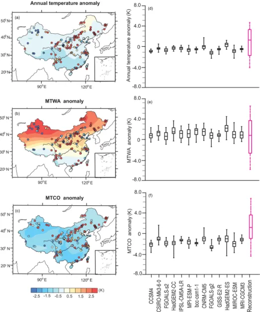
Based on pollen records, the spatial pattern of climate changes over China during the MH, deduced from IVM, are presented in Fig. 3a–c (points), alongside the results from PMIP3 models (shaded in Fig. 3). For temperature, a warmer-than-present annual climate condition (∼ 0.7 K on average) is derived from pollen data (the points in Fig. 3a), with the largest increase occurring in the northeast (3–5 K) and a decrease in the northwest and on Tibetan Plateau. On the other hand, the results from a multi-model ensemble (MME) indicate a generally colder annual temperature (∼ −0.4 K on average), with significant cooling in the south and slight warming in the northeast (shaded in Fig. 3a). Of the 13 models, 11 simulate a cooler annual temperature compared with PI than MME. However, two models (HadeGEM2-ES and CNRM-CM5) present the same warmer condition as was found in the reconstruction (Fig. 3d). Compared to the
re-Figure 2.Comparison of megabiomes for PI (a, c) and the MH (b, d): (a, b) BIOME6000 and (c, d) pollen data collected in this study.
construction, the annual mean temperature during the MH is largely underestimated by most PMIP3 models, which de-pict an anomaly ranging from ∼ −1 to ∼ 0.5 K. Concerning seasonal change, during the MH, MTWA from the data is ∼0.5 K higher than PI, with the largest increase in the north-east and a decrease in the northwest. From model outputs, an average increase of ∼ 1.2 K is reproduced by MME, with more pronounced warming at high latitudes, which is con-sistent with the insolation change (Berger, 1978). Figure 3e shows that all 13 models reproduce the same warmer summer temperatures as the data and that HadGEM2-ES and CNRM-CM5 reproduce the largest increases among the models. Al-though models simulate warmer MTWA, which is consistent with reconstructions, there is a discrepancy between them on MTCO. In Fig. 3c, the data show an overall increase of ∼1 K, with the largest increase occurring in the northeast and a decrease of opposite magnitude on the Tibetan Plateau. Inversely, MME reproduces a decreased MTCO with an av-erage amplitude of ∼ −1.3 K, the areas with strongest cool-ing becool-ing the southeast, the Loess Plateau and the north-west. Similarly to the MME, all 13 models simulate a colder-than-present climate with amplitudes ranging from ∼ −2.0 K (CCSM4 and FGOALS-g2) to ∼ −0.7 K (HadGEM2-ES and CNRM-CM5).
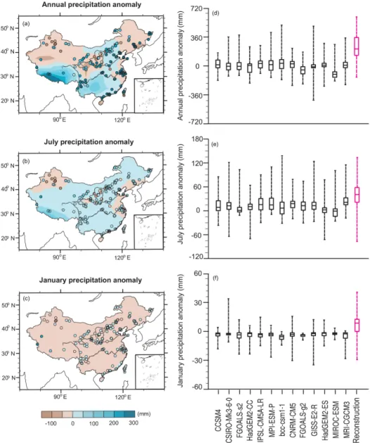
Concerning the annual change in precipitation, the recon-struction shows wetter conditions during the MH across
al-most the whole of China with the exception of part of the northwest. The southeast presents the largest increase in an-nual precipitation. All but two models (MIROC-ESM and FGOALS-g2) depict wetter conditions with an amplitude of ∼10 to ∼ 50 mm. The reconstruction and MME results also indicate an increased annual precipitation during the MH (Fig. 4a), with a much larger magnitude visible in the recon-struction (∼ 30 mm and ∼ 230 mm, respectively). The main discrepancy in annual precipitation between simulations and reconstruction occurs in the northeast, which is depicted as drier by the models and wetter by the data. With regard to seasonal change, the reconstruction shows an overall increase in July rainfall (∼ 50 mm on average), with a decrease in the northwestern regions and East Asian monsoon region in the Yangtze River valley. In line with the reconstruction, the MME also shows an overall increase in rainfall (∼ 7 mm on average), with a decrease in the northwest for July (Fig. 4b). Notably, a much larger increase is simulated for the south and the Tibetan Plateau by the models, while the opposite pattern emerges along the eastern margin from both models and data. For January precipitation, the reconstruction shows an overall increase in most regions (∼ 15 mm), except for the northwestern region, while MME indicates a slight decrease (∼ 3 mm on average). More detailed information about the geographic distribution of simulated temperature and precip-itation for each model can be found in Figs. S2–S7.
Figure 3.Model–data comparison for annual and seasonal (MTWA and MTCO) temperature (K). For (a–c), points represent the reconstruc-tion from IVM, and shading shows the last 30-year mean simulareconstruc-tion results of a multi-model ensemble (MME) for 13 PMIP3 models. The box-and-whisker plots (d–f) show the changes as indicated by each PMIP3 model and the reconstruction. (d) Changes in annual temperature, (e) changes in MTWA and (f) changes in MTCO. The lines in each box show the median value from each set of measurements, the box shows the 25 %–75 % range and the whiskers show the 90 % interval (5th to 95th percentile).
Table S4 provides the biome scores from IVM for pollen data collected from published papers. The reconstructed cli-mate change derived from IVM at each pollen site can be found in Table S5, in which the columns show the median and the 90 % interval (5th to 95th percentage) for feasible climate values produced with the IVM approach. The simu-lated values for each of the climate variables as shown in the box plots (Figs. 3 and 4) are given in Tables S6 and S7. All the values mentioned above are the mean of the values at 159 pollen sites.
3.2 Comparison of vegetation change at the MH
The use of the PMIP3 database is clearly limited by the dif-ferent vegetation inputs among the models for the MH pe-riod (Table S8). Only HadGEM2-ES and HadGEM2-CC use dynamic vegetation for the MH, and the vegetation of the other 11 models is prescribed to PI with or without inter-active leaf area index (LAI), which can introduce a bias to the role of vegetation–atmosphere interaction in the MH cli-mates. To evaluate the model results against the reconstruc-tion for the MH vegetareconstruc-tion, we conducted 13 biome simu-lations with BIOME4 using the PMIP3 climate fields, and the megabiome distribution for each model during the MH
Figure 4.Model–data comparison for annual, July and January precipitation (mm). For (a, b), points represent the reconstruction from IVM, and shading shows the last 30-year mean simulation results of a multi-model ensemble (MME) for 13 PMIP3 models. The box-and-whisker plots (d–f) show the changes as indicated by each PMIP3 model and the reconstruction. (d) Changes in annual precipitation, (e) changes in July precipitation and (f) changes in January precipitation. The lines in each box show the median value from each set of measurements, the box shows the 25 %–75 % range and the whiskers show the 90 % interval (5th to 95th percentile).
is displayed in Fig. 5 (see Fig. S8 for a comparison of PI biomes). To quantify the model–data dissimilarity between megabiomes, a map-based statistic called 1V (Sykes et al., 1999; Ni et al., 2000) was applied here (see Sect. 2.4).
Figure S9 shows the dissimilarity between simulations and observations for megabiomes during the MH, with the over-all values for 1V ranging from 0.43 (HadGEM2-ES) to 0.55 (IPSL-CM5A-LR). According to the classification of 1V (see Sect. 2.4) for the 13 models, 12 (all except HadGEM2-ES) showed poor agreement with the observed vegetation distribution. Most models poorly simulate the desert, grass-land and tropical forest areas for both periods but perform better for warm mixed forest, tundra and temperate forest.
However, this statistic is based on a point-to-point compari-son, so the 1V calculated here cannot represent an estima-tion of full vegetaestima-tion simulaestima-tion due to the uneven distribu-tion of pollen data and the potentially huge difference in the area of each megabiome. For instance, tundra in our data for PI is represented by only 4 points, which counts for a small contribution to 1V since we averaged it over a total of 159 points, but this calculation could induce a significant bias if these 4 points are representative of a large area of China.
So, we used the biome scores based on the artificial neural network technique as described by Guiot et al. (1996) for in-terpolation (the plots in the red rectangle in Fig. 5) and com-pared the simulated vegetation distribution from BIOME4
Figure 5.Comparison of interpolated megabiome distributions (plot in the red rectangle) with the simulated spatial pattern from BIOME4 for each model during the mid-Holocene.
for each model with the interpolated pattern. During the MH, most models are able to capture the tundra on the Tibetan Plateau as well as the combination of warm mixed forest and temperate forest in the southeast. However, all models fail to simulate or underestimate the desert area in the north-west compared to reconstructed data. The main model–data inconsistency in the MH vegetation distribution occurs in the northeast, where data show a mix of grassland and temperate forest, and the models show a mix of grassland and boreal forest.
The area statistics carried out for simulated vegetation changes (Fig. 6) reveal that the main difference during the MH, compared with PI, is that grassland replaced boreal for-est in large tracts of the northeast (Figs. 5, S8). No other
sig-nificant difference in vegetation distribution between the two periods was derived from the models. Unlike in the models, three main changes in megabiomes during the MH are de-picted by the data. Firstly, the megabiomes were converted from grassland to temperate forest in the northeast. Secondly, a large area of temperate forest was replaced in the southeast by a northward expansion of warm mixed forest. Thirdly, in the northwest and at the northern margin of the Tibetan Plateau, part of the desert area changed into grassland. How-ever, none of the models succeed in capturing these features, especially the transition from grassland into forest in the northeast during the MH. Therefore, this failure to capture vegetation changes between the two periods will lead to a cumulating inconsistency in the model–data comparison for
Figure 6.Changes in the extent of each megabiome as a consequence of simulated climate changes for each model, both expressed as change relative to the PI extent of the same megabiome.
climate anomalies if this computed vegetation was used as a boundary condition in MH climate simulations.
4 Discussion
4.1 Validation and uncertainties of the reconstructions
To investigate the discrepancy between models and recon-structions for the MH climate change over China, the reli-ability of our reconstruction should first be considered. We therefore compared our reconstruction with previous studies concerning the MH climate change over China based on mul-tiple proxies (including pollen, lake core, paleosol, ice core, peat and stalagmite); the related references and detailed in-formation are listed in the Supplement (Tables S9 and S10). In comparison with PI conditions, most reconstructions re-produced warmer and wetter annual conditions during the MH (Fig. 7), as in our study. In other words, this model– data discrepancy for climate change over China during the MH is common and robust with respect to reconstructions derived from different proxies. Our study reinforces the pic-ture given by the discrepancies between PMIP simulations and pollen data based on a synthesis of the literature.
However, there could still be some biases due to the re-construction method. Estimated climates for the present day from IVM were compared with observed climates (Table 6). The slopes and intercepts show a slight bias for annual and January precipitation, while there is a larger bias between the IVM reconstruction and observation for temperature and July precipitation. IVM relies heavily on BIOME4, and since BIOME4 is a global vegetation model, it is possible that the spatial robustness of regional reconstruction could be less than that of global reconstruction due to the failure to simulate local features (Bartlein et al., 2011). Moreover, the output of the model cannot be directly compared to the pollen data, and the conversion of BIOME4 biomes to pollen biomes by the transfer matrix may add a source of uncer-tainty in the reconstruction. All these biases in reconstruction should be considered in the evaluation of the discrepancy be-tween models and data for climate change during the MH over China.
4.2 Uncertainties for simulations
The discrepancies between models and data for MH climate change can also result from uncertainties in simulation and/or
Figure 7.Comparison between the climate reconstruction and previous reconstruction over China. (a) Previous temperature results. The diamond is the qualitative reconstruction, red is the temperature increase and green is the temperature decrease; the circle is the quantitative reconstruction. (b) Mean annual temperature reconstruction in this study; (c) previous precipitation results. The diamond is the qualitative reconstruction, red is the precipitation decrease and green is the precipitation increase; the circle is the quantitative reconstruction. (d) Mean annual precipitation reconstruction in this study.
model characteristics. First, the coarse spatial resolution of models can be a factor of discrepancy: previous studies show that the GCMs from PMIP3 are reliable in simulating the ge-ographical distribution of temperature and precipitation over China for the present day. However, compared with obser-vations, most models have topography-related cold biases (Jiang et al., 2016). The climate fields, directly used from the model output without downscaling, will not contain the spatial variability of modern climate in topographically com-plex areas. Thus, it is necessary to determine to what de-gree model–data mismatch is related to the rough topogra-phy used in the climate models. In PMIP3, MRI-CGCM3 has the highest resolution (atmosphere: 320 × 160 × L48; ocean: 364 × 368 × L51), while IPSL-CM5A-LR has the lowest (atmosphere: 96 × 96 × L39; ocean: 182 × 149 × L31). In Fig. 8, we give the actual modern topography and the inter-polated topography used in MRI-CGCM3 and IPSL-CM5A-LR. For MRI-CGCM3, the topography is very close to the observation, so for this model, the model–data discrepancy during the MH over China is not related to the
resolu-tion. However, for the model with coarse resolution (IPSL-CM5A-LR), it is true that the coarse version of the model will lead to a bias in topography when regional diversity is discussed. The spatial variations in topography could in-fluence the vegetation and hence the simulated climate. To quantify this impact, we compare the topography and PI cli-mate results of IPSL-CM5A-LR and IPSL-CM5A-MR. Fig-ure 9 shows that the difference in topography caused by model resolution does have an impact on small scales (e.g. southern region of the Tibetan Plateau) but not on the overall pattern. However, small- or regional-scale variations in cli-mate can have a large impact on vegetation and hence recon-structed climate. For better comparison in the future work, downscaled climate variables should be considered.
Secondly, besides the qualitative consistency among mod-els caused by the protocol of PMIP3 experiments (Table 2), variability in the magnitude of anomalies between models is clearly illustrated by the box plots (Figs. 3 and 4), espe-cially for the temperature anomaly. Figure S10 demonstrates that there is no clear relationship between PI temperature and
Figure 8.The topography comparison between models and observations.
temperature anomaly (MH–PI). In other words, these dispar-ities in value or even pattern among models are not related to the difference in PI simulations in a simple manner; instead, they reflect the obvious differences in the response by the cli-mate models to the MH forcing, which raises the question of the magnitude of feedbacks among models.
As positive feedbacks between climate and vegetation are important to explain regional climate changes, the failure of the models to represent the amplitude and pattern of the observed vegetation differences (see Sect. 3.2) could am-plify and partly account for the model–data disparities in cli-mate change, mainly due to variations in the albedo. Because HadGEM2-ES and HadGEM2-CC are the only two mod-els in PMIP3 with a dynamic vegetation simulation for the MH, we focused on these models to examine the variations in vegetation fraction in the simulations. The main vegeta-tion changes during the MH demonstrated by HadGEM2-ES are an increased tree coverage (∼ 15 %) and a decreased bare soil fraction (∼ 6 %), while HadGEM2-CC depicts a ∼ 3 % decrease in tree fraction and a ∼ 1 % increase in bare soil (Fig. S11). We made a rough calculation of albedo vari-ance caused solely by vegetation change for both models and for our reconstruction based on the area fraction and
albedo value of each vegetation type (Betts, 2000; Bonfils et al., 2001; Oguntunde et al., 2006; Bonan, 2008). The overall albedo change from the vegetation reconstruction during the MH shows a ∼ 1.8 % decrease when snow free, with a much larger impact (∼ 4.2 % decrease) when snow covered. The results from HadGEM2-ES are highly consistent with the albedo changes from the reconstruction, featuring a ∼ 1.4 % (∼ 6.5 %) decrease without (with) snow, while HadGEM2-CC produces an increased albedo value during the MH (∼ 0.22 % for snow free, ∼ 1.9 % with snow cover), depend-ing on its vegetation simulation. Two ideas could be inferred from this calculation: (1) HadGEM2-ES is much better in simulating the MH vegetation changes than HadGEM2-CC, and (2) the failure by models to capture these vegetation changes will result in a much larger impact on winter albedo (with snow) than summer albedo (without snow). In conclu-sion, there is an obvious advantage of using AOVGCM in-stead of AOGCM when discussing the MH climate, but the premise is that the AOVGCM can simulate an accurate veg-etation distribution.
These surface albedo changes due to vegetation changes could have a cumulative effect on the regional climate by modifying the radiative fluxes. For instance, the spread of
Figure 9.The pre-industrial climate comparison between simulations and observations. “Tas” means temperature 2 m above the surface, and “pr” means precipitation.
trees into the grassland biome in the northeast during the MH, revealed by the reconstruction in our study, should act as a positive feedback to climate warming by increasing the surface net shortwave radiation associated with reductions in albedo due to taller and darker canopies (Chapin et al., 2005). Previous studies show that cloud and surface albedo feed-backs on radiation are major drivers of differences between model outputs for past climates. Moreover, the land surface feedback shows large disparities among models (Braconnot and Kageyama, 2015).
We used a simplified approach (Taylor et al., 2007) to quantify the feedbacks and to compare model behaviour for the MH, thus justifying the focus on surface albedo and at-mospheric scattering (mainly accounting for cloud change). Surface albedo and cloud change are calculated using the simulated incoming and outgoing radiative fluxes at the Earth’s surface and at the top of the atmosphere (TOA) based on data for the last 30 years averaged from all models. Us-ing this framework, we quantified the effect of changes in albedo on the net shortwave flux at TOA (Braconnot and Kageyama, 2015) and further investigated the relationship between these changes and temperature change. Figure 10 shows that most models produced a negative cloud cover and surface albedo feedback on the annual mean shortwave ra-diative forcing. Concerning seasonal change, the shortwave cloud and surface feedback in most models tend to counter-act the insolation forcing during the boreal summer, while
they enhance the solar forcing during winter. A strong pos-itive correlation between albedo feedback and temperature change is depicted, with a large spread in the models ow-ing to the difference in albedo in the 13 models. In particu-lar, CNRM-CM5 and HadGEM2-ES capture higher values of cloud and surface albedo feedback, which could be the rea-son for the reversal of the decreased annual temperature seen in other models (Fig. 3d).
However, the vegetation patterns produced by BIOME4 in Fig. 5 are not used in the PMIP3 experimental set-up. They are only determined by the input variables from mod-els. Therefore, the disagreements on the MH vegetation pat-tern are possibly inherited from the PI. To better quantify the vegetation–climate feedback, two experiments were con-ducted in CESM version 1.0.5, including a mid-Holocene (MH) experiment (6 ka) with the original vegetation setting (prescribed as PI vegetation for the MH) and an MH experi-ment with reconstructed vegetation (6 ka_VEG). Figure 11 shows the climate anomalies (6 ka_VEG minus 6 ka) be-tween two simulations for both the annual and seasonal scale. For temperature, it is clear that the 6 ka_VEG simulation re-produces a warmer annual mean climate (∼ 0.3 K on age) as well as an obviously warmer winter (∼ 0.6 K on aver-age). For precipitation, the reconstructed vegetation leads to more annual and seasonal precipitation, which can also rec-oncile the model–data discrepancy of an increased amplitude for precipitation during the MH (the data reproduced a larger
Figure 10.Scatter plots showing temperature, cloud cover feedback and surface albedo feedback changes during the MH. The values shown are the simulated 30-year mean anomaly (MH–PI) for the 13 models. (a) Annual mean temperature relative to the annual mean cloud cover feedback and (d) annual surface albedo feedback. (b) Summer (JJA) mean temperature relative to the summer mean cloud cover feedback and (e) summer surface albedo feedback. (c) Winter (DJF) mean temperature relative to the summer mean cloud cover feedback and (f) winter surface albedo feedback. The horizontal and vertical lines in the plots represent the value of 0.
Figure 11. Climate anomalies between the two experiments (6 ka and 6 ka_VEG) conducted in CESM version 1.0.5. The anomalies (6 ka_VEG-6 ka) of temperature and precipitation at both the annual and seasonal scale are presented, and all these climate variables are calculated as the last 50-year means from two simulations.
amplitude than the model, as revealed by our study). So the mismatch between models and data in terms of MH vegeta-tion could partly account for the discrepancy in climate due to the interaction between vegetation and climate through ra-diative and hydrological forcing with albedo. These results highlight the value of building a new generation of models able to capture not only the atmosphere and ocean response, but also the non-linear responses of vegetation and hydrology to climate change.
5 Conclusion
In this study, we compare the annual and seasonal outputs from the PMIP3 models with an updated synthesis of climate reconstructions over China, including, for the first time, the seasonal cycle of temperature and precipitation. In response to the seasonal insolation change prescribed in PMIP3 for the MH, all models produce similar large-scale patterns for sea-sonal temperature and precipitation (higher than present July precipitation and MTWA, lower than present MTCO). The main discrepancy emerging from the model–data
compari-son occurs for the mean annual temperature and MTCO; data show an increased value and most models simulate the op-posite except CNRM-CM5 and HadGEM2-ES, which repro-duced the higher-than-present MH annual temperature. By conducting simulations with BIOME4 and CESM, we show that surface processes are the key factors explaining the dis-crepancies between models and data. These results show the importance of including the non-linear responses of the sur-face water and energy balance related to vegetation changes. However, it should also be noted that prescribing the veg-etation with reconstructed biomes would reduce the power of the biome-based climate reconstruction owing to the po-tential circularity (prescribe the vegetation to get the vegeta-tion). Moreover, besides the vegetation influence, the impact of rough topography, soil type and other possible factors on model–data discrepancy remains to be investigated in future work.
Data availability. The PMIP3 output is publicly available on the PMIP website (http://pmip3.lsce.ipsl.fr/, last access: 21 June 2019). The 65 pollen biomization results are provided by the Members of the China Quaternary Pollen Database (CQPD). Table 1 shows the information (including references) on the 91 collected pollen records and 3 original ones in our study; the biome scores of these 94 pollen records derived from IVM are listed in Table S4, and the digitized data on pollen can be requested from Qin Li ([email protected]). All the reconstructed climate values at each pollen site from IVM are provided in Table S5. For the data from CQPD, the basic information (location, data supporter, age control and biome type of each site) can be found in CQPD (2000), while the original data are not publicly available yet. These data can be requested from Yunli Luo ([email protected]; Institute of Botany, Chinese Academy of Sciences, Beijing, 100093, China), a core member and academic secretary of the CQPD.
Supplement. The supplement related to this article is available online at: https://doi.org/10.5194/cp-15-1223-2019-supplement.
Author contributions. YL carried out the model–data analysis and prepared the first draft, GR contributed a lot to the paper’s structure and content, and HW provided the reconstruction results from IVM and contributed the paper’s structure and content. RRS conducted the BIOME4 simulations. RZ carried out the simulation in CESM. PB, MK and ZG contributed great ideas on model–data comparison work. QL and YL provided pollen data. All co-authors helped to improve the paper.
Competing interests. The authors declare that they have no con-flict of interest.
Acknowledgements. We acknowledge the Paleoclimate Mod-elling Intercomparison Project and World Climate Research
Pro-gram’s Working Group on Coupled Modelling, which is responsi-ble for PMIP–CMIP, and we thank the climate modelling groups for producing and making available their model output. We are grate-ful to Marie-France Loutre, Patrick Bartlein and three anonymous reviewers for constructive comments. This research has been sup-ported by the Sino-French Caiyuanpei Program, the Bairen Pro-grams of the Chinese Academy of Sciences and the JPI-Belmont PACMEDY project (grant no. ANR-15-JCLI-0003-01). We also ac-knowledge Labex L-IPSL, funded by the French Agence Nationale de la Recherche (grant no. ANR-10-LABX-0018), for its support for the biome modelling based on the PMIP database.
Financial support. This research has been supported by the National Basic Research Program of China (grant no. 2016YFA0600504) and the National Science Foundation of China (grant nos. 41572165, 41690114 and 41125011).
Review statement. This paper was edited by Marie-France Loutre and reviewed by Patrick Bartlein and three anonymous ref-erees.
References
An, C., Zhao, J., Tao, S., Lv, Y., Dong, W., Li, H., Jin, M., and Wang, Z.: Dust variation recorded by lacustrine sediments from arid Central Asia since ∼ 15 cal ka BP and its implication for atmospheric circulation, Quaternary Res., 75, 566–573, 2011. Bao, Q., Lin, P., Zhou, T., Liu, Y., Yu, Y., Wu, G., He, B., He, J., Li,
L., Li, J., Li, Y., Liu, H., Qiao, F., Song, Z., Wang, B., Wang, J., Wang, P., Wang, X., Wang, Z., Wu, B., Wu, T., Xu, Y., Yu, H., Zhao, W., Zheng, W., and Zhou, L.: The flexible global ocean-atmosphere-land system model, spectral version 2: FGOALS-s2, Adv. Atmos. Sci., 30, 561–576, 2013.
Bartlein, P. J., Harrison, S. P., Brewer, S., Connor, S., Davis, B. A. S., Gajewski, K., Guiot, J., Harrison-Prentice, T. I., Henderson, A., Peyron, O., Prentice, I. C., Scholze, M., Seppä, H., Shuman, B., Sugita, S., Thompson, R. S., Viau, A. E., Williams, J., and Wu, H. B.: Pollen-based continental climate reconstructions at 6 and 21 ka: a global synthesis, Clim. Dynam., 37, 775–802, 2011. Berger, A.: Long-Term Variations of Daily Insolation and
Quater-nary Climatic Changes, J. Atmos. Sci., 35, 2362–2367, 1978. Betts, R. A.: Offset of the potential carbon sink from boreal
foresta-tion by decreases in surface albedo, Nature, 408, 187–190, 2000. Bigelow, N. H., Brubaker, L. B., Edwards, M. E., Harrison, S. P., Prentice, I. C., Anderson, P. M., Andreev, A. A., Bartlein, P. J., Christensen, T. R., Cramer, W., Kaplan, J. O., Lozhkin, A. V., Matveyeva, N. V., Murray, D. F., David McGuire, A., Razzhivin, V. Y., Ritchie, J. C., Smith, B., Walker, A. D., Gajewski, K., Wolf, V., Holmqvist, B. H., Igarashi, Y., Kremenetskii, K., Paus, A., Pisaric, M. F. J., and Volkova, V. S.: Climate change and Arctic ecosystems: 1. Vegetation changes north of 55◦N between the last glacial maximum, mid-Holocene and present, J. Geophys. Res., 108, 1–25, 2003.
Bonan, G. B.: Forests and Climate Change: Forcings, Feedbacks, and the Climate Benefits of Forests, Science, 320, 1444–1449, 2008.
Bonfils, C., de Noblet-Ducoudré, N., Braconnot, P., and Joussaume, S.: Hot Desert Albedo and Climate Change: Mid-Holocene Mon-soon in North Africa, J. Climate, 14, 3724–3737, 2001. Braconnot, P. and Kageyama, M.: Shortwave forcing and feedbacks
in Last Glacial Maximum and Mid-Holocene PMIP3 simula-tions, Philos. T. R. Soc. A, 373, 2054–2060, 2015.
Braconnot, P., Otto-Bliesner, B., Harrison, S., Joussaume, S., Pe-terchmitt, J.-Y., Abe-Ouchi, A., Crucifix, M., Driesschaert, E., Fichefet, Th., Hewitt, C. D., Kageyama, M., Kitoh, A., Laîné, A., Loutre, M.-F., Marti, O., Merkel, U., Ramstein, G., Valdes, P., Weber, S. L., Yu, Y., and Zhao, Y.: Results of PMIP2 coupled simulations of the Mid-Holocene and Last Glacial Maximum – Part 1: experiments and large-scale features, Clim. Past, 3, 261– 277, https://doi.org/10.5194/cp-3-261-2007, 2007a.
Braconnot, P., Otto-Bliesner, B., Harrison, S., Joussaume, S., Pe-terchmitt, J.-Y., Abe-Ouchi, A., Crucifix, M., Driesschaert, E., Fichefet, Th., Hewitt, C. D., Kageyama, M., Kitoh, A., Loutre, M.-F., Marti, O., Merkel, U., Ramstein, G., Valdes, P., Weber, L., Yu, Y., and Zhao, Y.: Results of PMIP2 coupled simula-tions of the Mid-Holocene and Last Glacial Maximum – Part 2: feedbacks with emphasis on the location of the ITCZ and mid- and high latitudes heat budget, Clim. Past, 3, 279-296, https://doi.org/10.5194/cp-3-279-2007, 2007b.
Braconnot, P., Harrison, S. P., Kageyama, M., Bartlein, P. J., Masson-Delmotte, V., Abe-Ouchi, A., Otto-Bliesner, B., and Zhao, Y.: Evaluation of climate models using palaeoclimatic data, Nat. Clim. Change, 2, 417–421, 2012.
Cai, Y.: Study on environmental change in Zoige Plateau: Evidence from the vegetation record since 24000 a B.P., Chinese Academy of Geological Sciences, Mater Dissertation, 2008 (in Chinese with English abstract).
Caudill, M. and Bulter, C.: Understanding Neural Networks, Basic Networks, 1, 309–331, 1992.
Chapin, F. S., Sturm, M., Serreze, M. C., McFadden, J. P., Key, J. R., Lloyd, A. H., McGuire, A. D., Rupp, T. S., Lynch, A. H., Schimel, J. P., Beringer, J., Chapman, W. L., Epstein, H. E., Eu-skirchen, E. S., Hinzman, L. D., Jia, G., Ping, C.L., Tape, K. D., Thompson, C. D. C., Walker, D. A., and Welker, J. M.: Role of Land-Surface Changes in Arctic Summer Warming, Science, 310, 657–660, 2005.
Chen, F., Cheng, B., Zhao, Y., Zhu, Y., and Madsen, D. B.: Holocene environmental change inferred from a high-resolution pollen record, Lake Zhuyeze, arid China, The Holocene, 16, 675–684, 2006.
Chen, F., Xu, Q., Chen, J., Birks, H. J. B., Liu, J., Zhang, S., Jin, L., An, C., Telford, R. J., Cao, X., Wang, Z., Zhang, X., Selvaraj, K., Lu, H., Li, Y., Zheng, Z., Wang, H., Zhou, A., Dong, G., Zhang, J., Huang, X., Bloemendal, J., and Rao, Z.: East Asian summer monsoon precipitation variability since the last deglaciation, Sci. Rep., 5, 1–11, 2015.
Cheng, B., Chen, F., and Zhang, J.: Palaeovegetational and Palaeoenvironmental Changes in Gonghe Basin since Last Deglaciation, Ac. Geogr. Sin., 11, 1336–1344, 2010 (in Chinese with English abstract).
Cheng, H., Edwards, R. L., Sinha, A., Spötl, C., Yi, L., Chen, S., Kelly, M., Kathayat, G., Wang, X., Li, X., Kong, X., Wang, Y., Ning, Y., and Zhang, H.: The Asian monsoon over the past 640,000 years and ice age terminations, Nature, 534, 640–646, 2016.
Cheng, Y.: Vegetation and climate change in the north-central part of the Loess Plateau since 26,000 years, China University of Geosciences, Master Dissertation, 2011 (in Chinese with English abstract).
Collins, W. J., Bellouin, N., Doutriaux-Boucher, M., Gedney, N., Halloran, P., Hinton, T., Hughes, J., Jones, C. D., Joshi, M., Lid-dicoat, S., Martin, G., O’Connor, F., Rae, J., Senior, C., Sitch, S., Totterdell, I., Wiltshire, A., and Woodward, S.: Development and evaluation of an Earth-System model – HadGEM2, Geosci. Model Dev., 4, 1051–1075, https://doi.org/10.5194/gmd-4-1051-2011, 2011.
Cui, M., Luo, Y., and Sun, X.: Paleovegetational and paleoclimatic changed in Ha’ni Lake, Jilin since 5 ka BP, Mar. Geol. Quatern. Geol., 26, 117–122, 2006 (in Chinese with English abstract). Dallmeyer, A., Claussen, M., Ni, J., Cao, X., Wang, Y., Fischer, N.,
Pfeiffer, M., Jin, L., Khon, V., Wagner, S., Haberkorn, K., and Herzschuh, U.: Biome changes in Asia since the mid-Holocene – an analysis of different transient Earth system model simu-lations, Clim. Past, 13, 107–134, https://doi.org/10.5194/cp-13-107-2017, 2017.
Davis, B. A. S., Brewer, S., Stevenson, A. C., and Guiot, J.: The temperature of Europe during the Holocene reconstructed from pollen data, Quaternary Sci. Rev., 22, 1701–1716, 2003. Diffenbaugh, N. S., Sloan, L. C., Snyder, M. A., Bell, J. L.,
Ka-plan, J., Shafer, S. L., and Bartlein, P. J.: Vegetation sensitiv-ity to global anthropogenic carbon dioxide emissions in a topo-graphically complex region, Global Biogeochem. Cy., 17, 1067, https://doi.org/10.1029/2002GB001974, 2003.
Dufresne, J. L., Foujols, M. A., Denvil, S., Caubel, A., Marti, O., Aumont, O., Balkanski, Y., Bekki, S., Bellenger, H., Ben-shila, R., Bony, S., Bopp, L., Braconnot, P., Brockmann, P., Cadule, P., Cheruy, F., Codron, F., Cozic, A., Cugnet, D., No-blet, N., Duvel, J.P., Ethe, C., Fairhead, L., Fichefet, T., Flavoni, S., Friedlingstein, P., Grandpeix, J. Y., Guez, L., Guilyardi, E., Hauglustaine, D., Hourdin, F., Idelkadi, A., Ghattas, J., Jous-saume, S., Kageyama, M., Krinner, G., Labetoulle, S., Lahel-lec, A., Lefevre, M.-F., Lefevre, F., Levy, C., Li, Z. X., Lloyd, J., Lott, F., Madec, G., Mancip, M., Marchand, M., Masson, S., Meurdesoif, Y., Mignot, J., Musat, I., Parouty, S., Polcher, J., Rio, C., Schulz, M., Swingedouw, D., Szopa, S., Talandier, C., Terray, P., Viovy, N., and Vuichard, N.: Climate change projections us-ing the IPSL-CM5 Earth system model: from CMIP3 to CMIP5, Clim. Dynam., 40, 2123–2165, 2013.
EPICA Community Members: Eight glacial cycles from an Antarc-tic ice core, Nature, 429, 623–628, 2004.
Food and Agricultural Organization: Soil Map of the World 1 : 5 000 000, FAO, 1995.
Farrera, I., Harrison, S. P., Prentice, I. C., Ramstein, G., Guiot, J., Bartlein, P. J., Bonnefille, R., Bush, M., Cramer, W., von Grafen-stein, U., Holmgren, K., Hooghiemstra, H., Hope, G., Jolly, D., Lauritzen, S. E., Ono, Y., Pinot, S., Stute, M., and Yu, G.: Trop-ical climates at the Last Glacial Maximum: a new synthesis of terrestrial palaeoclimate data. I. Vegetation, lake-levels and geo-chemistry, Clim. Dynam., 15, 823–856, 1999.
Fischer, N. and Jungclaus, J. H.: Evolution of the seasonal tempera-ture cycle in a transient Holocene simulation: orbital forcing and sea-ice, Clim. Past, 7, 1139–1148, https://doi.org/10.5194/cp-7-1139-2011, 2011.