HAL Id: hal-02873932
https://hal.archives-ouvertes.fr/hal-02873932
Submitted on 22 Jun 2020
HAL is a multi-disciplinary open access
archive for the deposit and dissemination of
sci-entific research documents, whether they are
pub-lished or not. The documents may come from
teaching and research institutions in France or
abroad, or from public or private research centers.
L’archive ouverte pluridisciplinaire HAL, est
destinée au dépôt et à la diffusion de documents
scientifiques de niveau recherche, publiés ou non,
émanant des établissements d’enseignement et de
recherche français ou étrangers, des laboratoires
publics ou privés.
using radioactive tracers of opportunity and an ensemble
of 19 global models
I. N. Kristiansen, A. Stohl, D. J. L. Olivié, B. Croft, O. A. Søvde, H. Klein, T.
Christoudias, D. Kunkel, J. Leadbetter S., H. Lee Y., et al.
To cite this version:
I. N. Kristiansen, A. Stohl, D. J. L. Olivié, B. Croft, O. A. Søvde, et al.. Evaluation of observed
and modelled aerosol lifetimes using radioactive tracers of opportunity and an ensemble of 19 global
models. Atmospheric Chemistry and Physics, European Geosciences Union, 2016, 16, pp.3525 - 3561.
�10.5194/acp-16-3525-2016�. �hal-02873932�
www.atmos-chem-phys.net/16/3525/2016/ doi:10.5194/acp-16-3525-2016
© Author(s) 2016. CC Attribution 3.0 License.
Evaluation of observed and modelled aerosol lifetimes using
radioactive tracers of opportunity and an ensemble
of 19 global models
N. I. Kristiansen1, A. Stohl1, D. J. L. Olivié2, B. Croft3, O. A. Søvde4, H. Klein2, T. Christoudias5, D. Kunkel6, S. J. Leadbetter7, Y. H. Lee8, K. Zhang9, K. Tsigaridis10, T. Bergman11, N. Evangeliou1,12, H. Wang9, P.-L. Ma9, R. C. Easter9, P. J. Rasch9, X. Liu13, G. Pitari14, G. Di Genova14, S. Y. Zhao15, Y. Balkanski12, S. E. Bauer10, G. S. Faluvegi10, H. Kokkola11, R. V. Martin3, J. R. Pierce16,3, M. Schulz2, D. Shindell8, H. Tost6, and H. Zhang15
1NILU – Norwegian Institute for Air Research, Kjeller, Norway 2Norwegian Meteorological Institute, Oslo, Norway
3Department of Physics and Atmospheric Science, Dalhousie University, Halifax, Canada 4Center for International Climate and Environmental Research – Oslo (CICERO), Oslo, Norway 5The Cyprus Institute, Nicosia, Cyprus
6Institute for Atmospheric Physics, Johannes Gutenberg University of Mainz, Mainz, Germany 7Met Office, Exeter, UK
8Earth and Ocean Sciences, Nicholas School of the Environment, Duke University, Durham, NC, USA 9Pacific Northwest National Laboratory (PNNL), Richland, WA, USA
10Center for Climate Systems Research, Columbia University, and NASA Goddard Institute for Space Studies, New York, NY, USA
11Finnish Meteorological Institute, Kuopio, Finland
12Laboratoire des Sciences du Climat et de l’Environnement, CEA-CNRS-UVSQ, Gif-sur-Yvette, France 13Department of Atmospheric Science, University of Wyoming, Laramie, WY, USA
14University of L’Aquila, L’Aquila, Italy
15Laboratory for Climate Studies, National Climate Center, Chinese Meteorological Administration, Beijing, China 16Department of Atmospheric Science, Colorado State University, Fort Collins, CO, USA
Correspondence to: N. I. Kristiansen (nik@nilu.no)
Received: 5 August 2015 – Published in Atmos. Chem. Phys. Discuss.: 9 September 2015 Revised: 29 February 2016 – Accepted: 2 March 2016 – Published: 17 March 2016
Abstract. Aerosols have important impacts on air quality and
climate, but the processes affecting their removal from the at-mosphere are not fully understood and are poorly constrained by observations. This makes modelled aerosol lifetimes un-certain. In this study, we make use of an observational con-straint on aerosol lifetimes provided by radionuclide mea-surements and investigate the causes of differences within a set of global models. During the Fukushima Dai-Ichi nu-clear power plant accident of March 2011, the radioactive isotopes cesium-137 (137Cs) and xenon-133 (133Xe) were re-leased in large quantities. Cesium attached to particles in the ambient air, approximately according to their available
aerosol surface area.137Cs size distribution measurements taken close to the power plant suggested that accumulation-mode (AM) sulfate aerosols were the main carriers of ce-sium. Hence,137Cs can be used as a proxy tracer for the AM sulfate aerosol’s fate in the atmosphere. In contrast, the no-ble gas133Xe behaves almost like a passive transport tracer. Global surface measurements of the two radioactive isotopes taken over several months after the release allow the deriva-tion of a lifetime of the carrier aerosol. We compare this to the lifetimes simulated by 19 different atmospheric transport models initialized with identical emissions of137Cs that were assigned to an aerosol tracer with each model’s default
prop-erties of AM sulfate, and133Xe emissions that were assigned to a passive tracer. We investigate to what extent the mod-elled sulfate tracer can reproduce the measurements, espe-cially with respect to the observed loss of aerosol mass with time. Modelled137Cs and 133Xe concentrations sampled at the same location and times as station measurements allow a direct comparison between measured and modelled aerosol lifetime. The e-folding lifetime τe, calculated from station measurement data taken between 2 and 9 weeks after the start of the emissions, is 14.3 days (95 % confidence interval 13.1–15.7 days). The equivalent modelled τelifetimes have a large spread, varying between 4.8 and 26.7 days with a model median of 9.4 ± 2.3 days, indicating too fast a removal in most models. Because sufficient measurement data were only available from about 2 weeks after the release, the estimated lifetimes apply to aerosols that have undergone long-range transport, i.e. not for freshly emitted aerosol. However, mod-elled instantaneous lifetimes show that the initial removal in the first 2 weeks was quicker (lifetimes between 1 and 5 days) due to the emissions occurring at low altitudes and co-location of the fresh plume with strong precipitation. De-viations between measured and modelled aerosol lifetimes are largest for the northernmost stations and at later time pe-riods, suggesting that models do not transport enough of the aerosol towards the Arctic. The models underestimate pas-sive tracer (133Xe) concentrations in the Arctic as well but to a smaller extent than for the aerosol (137Cs) tracer. This indi-cates that in addition to too fast an aerosol removal in the models, errors in simulated atmospheric transport towards the Arctic in most models also contribute to the underesti-mation of the Arctic aerosol concentrations.
1 Introduction
Aerosols play an important role in air quality and influence the global climate (Friedlander, 1977; Seinfeld and Pandis, 1998; Ramanathan et al., 2001) but the processes affect-ing their removal from the atmosphere are not fully under-stood and are poorly constrained by observations. Generally, aerosol concentrations are affected by emissions, transport, removal, and physico-chemical transformation (e.g. Pöschl, 2005), and the atmospheric lifetime of aerosols is a function of the various removal processes, such as dry deposition by impaction and sedimentation, as well as wet deposition. For accumulation-mode (AM) aerosols (0.1–2 µm diameter), the dominant removal process is wet deposition. The uncertain-ties and lack of observational constraints on these removal processes affect the ability to model aerosol concentrations correctly and make modelled aerosol lifetimes uncertain. The uncertainty in the effects of aerosols on climate further af-fects the ability to diagnose how sensitive the climate is to greenhouse gas emissions (e.g. Andreae, 2007).
Observation-based estimates of aerosol lifetimes are sparse due to the difficulty of obtaining measurements that cover a sufficient geographical area and time period for ro-bust analysis. Reported observation-based aerosol lifetimes range from a few days to about a month in the troposphere (Williams et al., 2002; Paris et al., 2009; Schmale et al., 2011). Other aerosol lifetime estimates are derived from ra-dionuclides produced by cosmic rays, radon decay, or nu-clear bomb tests, and vary from 4 days to more than a month (Giorgi and Chameides, 1986), reflecting the different origin (e.g. surface or stratospheric) of radionuclide tracers. Aerosol residence times of about 4 days in the lower troposphere and about 12 days in the middle to upper troposphere may be seen as typical (Moore et al., 1973), but higher values of 8 days for the lower troposphere have been reported as well (Papastefanou, 2006). Following the Chernobyl nuclear acci-dent, the exponential decline of the radionuclide concentra-tions indicated a residence time of 7 days (Cambray et al., 1987). Models report global average residence times of AM aerosol in the atmosphere on the order of 3–7 days for species emitted near the surface (Chin et al., 1996; Feichter et al., 1996; Stier et al., 2005; Berglen et al., 2004; Liu et al., 2005; Bourgeois and Bey, 2011; Chung and Seinfeld, 2002; Koch and Hansen, 2005; Textor et al., 2006). The differences in reported lifetimes from observations and models can partly be attributed to the applied definition of lifetime (i.e. char-acteristic time of exponential decay vs. ratio of burden to deposition or emissions). These lifetime definitions are only equivalent if the decay has a constant e-folding time over the considered time period (Croft et al., 2014). Several defini-tions of lifetime and residence time (the ratio of burden to deposition/emission/production) exist but the terminologies are often used inconsistently. We encourage future studies to give clear information about which lifetime definitions that are used.
Many modelling studies have analysed the global distribu-tion, transport, and lifetime of aerosols, particularly within the Aerosol Comparisons between Observations and Mod-els (AeroCom) initiative (e.g. Textor et al., 2006; Koch et al., 2009; Samset et al., 2014). It has been demonstrated that large differences exist for aerosol dispersal and removal be-tween models. Samset et al. (2014) found that, compared to aircraft measurements, models seem to overestimate black carbon (BC) aerosol concentrations in the middle and upper troposphere, and thus, a short aerosol lifetime appears neces-sary to reproduce such observations. On the other hand, the models generally underestimate the aerosol concentrations closer to the surface, and this would get worse with a shorter model lifetime. In particular, models struggle to capture the high aerosol concentrations in the Artic related to the Arctic haze season (e.g. Shindell et al., 2008; Koch et al., 2009). A general underestimation of surface aerosol concentrations in the Arctic is found during the Arctic haze season, while an overestimation is often found in the summer (e.g. Eckhardt et al., 2015). Models underestimate poleward transport,
re-move aerosols too efficiently, or do not confine pollution suf-ficiently to the lowest model levels due to excessive vertical diffusion (Koch et al., 2009), but it is not clear which is the main cause. It has also not been fully quantified how these model issues evolve during transport to the Arctic. Browse et al. (2012) and H. Wang et al. (2013) found that scavenging parameterizations play a significant role in modelling Arc-tic aerosol concentrations. In parArc-ticular, slow scavenging by ice clouds in winter and enhanced scavenging by drizzle in summer are important for modelling the annual cycle of Arc-tic aerosol concentrations. Using a source-tagging technique, H. Wang et al. (2014) found that the annual mean lifetime of Arctic AM BC aerosol has very strong source-region depen-dence, varying by a factor of 4. Zhang et al. (2015) further showed that the lifetime also depends on season and emis-sion type. Substantially lower BC lifetime is found in sum-mer, likely due to relatively strong wet removal, than in other seasons, and open-fire emissions that have higher initial in-jection heights which lead to generally longer lifetime than emissions from the surface.
In this study, we evaluate modelled aerosol lifetimes slightly differently than in previous studies. We use a unique single event with relatively well-known emissions to deter-mine the lifetime of aerosols in the atmosphere. Previous studies report the mean lifetime of aerosols from simulations with higher uncertainty in the emission terms. Specifically, emissions and lifetimes are sometimes tuned to obtain what are thought to be “reasonable” concentrations. In this exer-cise, we use emissions of radionuclides from the Fukushima Dai-Ichi nuclear power plant (FD-NPP) accident in March 2011 as “tracers of opportunity”. The cesium (137Cs) re-leased during the accident attached to the particles in the am-bient air, approximately in proportion to their surface area (Papastefanou, 2008). The peak of the aerosol surface area distribution is generally in the AM, which in the area of FD-NPP is typically dominated by sulfate. Kaneyasu et al. (2012) performed measurements close to FD-NPP and confirmed that137Cs was attached to or included in aerosols (internally mixed with other aerosol components), and their137Cs size distribution measurements showed that AM sulfate aerosols were the main transport carriers of cesium. They further ex-plained that elemental carbon (EC) or BC particles were un-likely to be the transport carriers because flaming fires did not continue during the FD-NPP accident, large-scale forest fires were not reported around FD-NPP, and because the local res-idents had refrained from the burning of firewood in fear of the re-emission of radionuclides since the accident. However, they could not exclude the possibility that water-insoluble or-ganic carbon (OC) could have acted as a transport medium of cesium. Even though it is possible that some of the137Cs attached to other aerosol than sulfate, these aerosol compo-nents were likely mixed internally with the dominant AM sulfate aerosol and therefore should have similar removal properties. Miyamoto et al. (2014) reported137Cs size distri-bution measurements taken in an earlier phase (6 days after
the accident) and closer to FD-NPP, which showed an activity median aerodynamic diameter (AMAD) of137Cs of around 1.5–1.6 µm, in agreement with the results of Kaneyasu et al. (2012). Masson et al. (2013) found that after long-range transport to Europe, the AMAD of 137Cs ranged between 0.25 and 0.71 µm, thus again in the AM of the ambient aerosols. Hence,137Cs can be used as a proxy tracer for the AM sulfate aerosol’s fate in the atmosphere.
Cesium from FD-NPP was measured in the Northern Hemisphere for more than 3 months after its release and traced the fate of its carrier-aerosol in the atmosphere. These measurements provided a unique opportunity to estimate the lifetime of AM aerosols in the atmosphere, as presented by Kristiansen et al. (2012). In that study, measurements of the two radionuclides xenon (133Xe) and cesium (137Cs) were used, both released in large quantities from FD-NPP. The noble gas xenon (133Xe) was used as a passive transport tracer. Notice that both radionuclides have very low back-ground concentrations caused by emissions from nuclear fa-cilities (Wotawa et al., 2010) or, in the case of137Cs, resus-pension of deposited radiocesium. Background values were subtracted from all measured values, as described by Kris-tiansen et al. (2012). These authors used the measured ratios of the aerosol (137Cs) to the passive tracer (133Xe) enhance-ments in the surface concentrations, to compensate for vari-ability in transport, and estimated an AM aerosol lifetime of 10–14 days. This is longer than the mean lifetimes of AM aerosols obtained from most aerosol models (typically in the range of 3–7 days). The disagreement could be partly due to the fact that the emissions were from a single location and during a specific season, the measurements were all ground-based, and thus the data were not fully representative of the global and annual mean aerosol lifetime, as well as using def-initions of lifetime that were not equivalent under the consid-ered conditions (Croft et al., 2014). In the current study, we try to resolve this issue and investigate to what extent aerosol models can reproduce the observations, especially with re-spect to the observed loss of aerosol mass with time.
We use the term “aerosol lifetime” throughout the paper to indicate the lifetime of AM aerosol and primarily sulfate. We assume that the137Cs attached mostly to the dominant AM sulfate aerosol, confirmed by measurements. The lifetimes apply to aerosols that have undergone long-range transport (after about 2–3 weeks); i.e. the results presented cannot di-rectly constrain the lifetime of freshly emitted aerosols.
The paper is organized as follows. In Sect. 2 we describe the measurements used in the study, followed by an overview of all participating models in Sect. 3. The methods are de-scribed in Sect. 4, and the main results are presented in Sect. 5. In Sect. 6 we further discuss some important aspects of the results and compare our results to other recent studies. Main conclusions are summarized in Sect. 7. The paper also includes supplementary information in three Appendices, A to C.
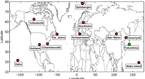
−150 −100 −50 0 50 100 150 10 20 30 40 50 60 70 80 Fukushima Wake Island Oahu Yellowknife Ashland Charlottesville St. Johns Schauinsland Spitsbergen Stockholm Ulan−Bator Ussuriysk Latitude Longitude
Figure 1. Measurement station network. CTBTO stations (red markers) measuring particulates (137Cs) and noble gases (133Xe). The position of the Fukushima Dai-Ichi nuclear power plant (FD-NPP) is shown by a green marker.
2 Observations
We have used atmospheric surface measurements of activity concentrations of the noble gas133Xe and the aerosol-bound radionuclide 137Cs available from several stations (Fig. 1) operated by the Comprehensive Nuclear-Test-Ban Treaty Organization (CTBTO). For collecting particulate radionu-clides, about 20 000 m3of air is blown through a filter over a period of 24 h. The different radionuclides are measured with high-resolution germanium detectors (Schulze et al., 2000; Medici, 2001). The minimum detectable activity concentra-tion of137Cs is 1 µBq m−3. During the International Noble Gas Experiment (INGE), noble gas measurement systems have been set up worldwide (Wernsberger and Schlosser, 2004; Saey and de Geer, 2005) at CTBTO stations. The col-lection period of the xenon samples is typically 12 h. The most prevalent and important isotope is133Xe, which is mea-sured with an accuracy of about 0.1 mBq m−3. All measured radionuclide concentrations were corrected for radioactive decay relative to the time of the earthquake on 11 March 05:46 UTC that triggered the nuclear accident. The measure-ments were further converted from activity per norm cubic metre at standard temperature and pressure (273.15 K and 101 325 Pa) to activity per cubic metre (using meteorologi-cal analysis data) for comparison with the model results. The measurements and their uncertainties are described in more detail by Stohl et al. (2012a) and Kristiansen et al. (2012).
3 Model simulations
A total of 19 atmospheric transport models have simulated the transport and removal of the radioactive isotopes released during the FD-NPP accident. The models are classified as either Lagrangian particle dispersion models (LPDMs),
aerosol transport models (ATMs; models which rely entirely on meteorological input data) and aerosol circulation mod-els (ACMs; modmod-els which calculate their own meteorology or are nudged towards (re)analysis data). Table 1 shows an overview of the models included in the experiment includ-ing their type, meteorology, and model resolutions. More de-tails on each model’s treatment of aerosols are given in Ap-pendix A, Table A1.
All model simulations were initiated with identical emis-sions of cesium (137Cs) and xenon (133Xe) as determined from inverse modelling by Stohl et al. (2012a). The simu-lations extended from 11 March until at least 5 June 2011 for when the last measurement of the radionuclides were taken. A total of 36.6 PBq of137Cs and 15.3 EBq of133Xe were released by all models. The emission rates vary sig-nificantly over the emission period considered (11 March– 20 April 2011) but the major emissions of the radionuclides occurred over about 5 days (11–15 March 2011). The emis-sions of cesium continued until 20 March after which they dropped significantly. The releases were divided into three vertical layers between 0 and 1000 m above ground level (Stohl et al., 2012a). Croft et al. (2014) have shown that the e-folding lifetimes derived from their GEOS-Chem model simulations of the Fukushima emissions do not depend very much on the exact specification of the emissions (e.g. their altitude, location, and time). This is because radionuclides could be measured in the atmosphere for several months, long after the emissions had practically ceased (Kristiansen et al., 2012). Therefore, after the end of the emissions the decrease in measured concentrations can be attributed solely to aerosol removal. Biases in the emissions affect the abso-lute model-simulated values, but not the lifetime estimate. In the analysis, it might be expected that the FLEXPART model will perform relatively well since the source terms used by all
Table 1. List of models. ATMs: aerosol transport models (models which rely entirely on meteorological input data), ACMs: aerosol
circula-tion models (models which calculate their own meteorology or are nudged towards (re)analysis data), LPDMs: Lagrangian particle dispersion models,∗AEROCOM Phase II models.
Model Type Meteorology Model output resolution
H: horizontal (degrees lat × long) V: vertical, T: temporal
References
1 NorESM ACM Internal (generated online) H: 1.875◦×2.5◦
V: 26 levels up to ∼ 2.2 hPa. T: 3 h mean (model calc. 30 min)
Kirkevåg et al. (2013), Iversen et al. (2013), Bentsen et al. (2013) 2 GISS-ModelE2-TOMAS∗ ACM NCEP reanalysis horizontal
winds every 6 h
H: 2.0◦×2.5◦ V: 40 levels up to 0.1 hPa T: 3 h mean (model calc. 30 min)
Adams and Seinfeld (2002); Lee et al. (2015)
3 GISS-ModelE∗ ACM NCEP reanalysis horizontal
winds every 6 h
H: 2.0◦×2.5◦ V: 40 levels up to 0.1 hPa T: 3 h mean (model calc. 30 min)
Koch et al. (2006); Tsigaridis et al. (2013); Schmidt et al. (2014)
4 ULAQ-CCM ACM Internal (generated online) H: 5.0◦×6.0◦(T21)
V: 126 levels up to mesosphere T: 45 min
Pitari et al. (2014)
5 BCC_AGCM_2.0.1_CAM∗ ACM Online coupled. NCEP/NCAR
reanalysis as initial field
H: 2.8◦×2.8◦ V: 26 levels up to 2.9 hPa T: 3 h (model calc. 20 min)
Gong et al. (2003); H. Zhang et al. (2012); H. Zhang et al. (2014)
6 LMDZORINCA ACM Nudged to ERA-Interim
reanal-ysis wind fields every 6 h with a relaxation time of 10 days
H: 2.5◦×1.27◦ V: 39 levels up to ∼ 78 km T: 3 h mean
Evangeliou et al. (2013)
7 CAM5∗ ACM ERA-Interim reanalysis every
6 h (re-gridded to the model grid resolution) H: 1.9◦×2.5◦ V: 56 levels up to 1.9 hPa T: 30 min Liu et al. (2012); Ma et al. (2013)
8 CAM5_PNNL∗ ACM Same as CAM5 Same as CAM5 H. Wang et al. (2013)
9 CAM5_NDG ACM ERA-Interim reanalysis
hori-zontal winds (re-gridded to the model grid) at every model time step, with a relaxation timescale of 6 h H: 1.9◦×2.5◦ V: 30 levels up to 3.6 hPa T: 30 min Liu et al. (2012); K. Zhang et al. (2014) 10 ECHAM5-MESSy-Atmospheric Chemistry Model, v1.92 (EMAC-1)
ACM ERA-Interim every 6 h on the model grid resolution. Nudged variables are divergence and vorticity of the wind, tempera-ture, and the logarithm of the surface pressure
H: 1.1◦×1.1◦ V: 31 levels up to 10 hPa T: 3 h (model calc. 6 min)
Christoudias and Lelieveld (2013)
11
ECHAM5-MESSy-Atmospheric Chemistry Model, v2.50 (EMAC-2)
ACM ERA-Interim every 6 h on the model grid resolution. Nudged variables are divergence and vorticity of the wind, tempera-ture, and the logarithm of the surface pressure
H: 1.9◦×1.9◦
V: 31 levels up to 10 hPa (∼ 30 km) T: 1 h (model calc. 15 min)
Kunkel (2012); Kunkel et al. (2013)
12 ECHAM5-HAM2∗ ACM Nudged towards ERA-Interim
reanalysis at every time step. Relaxation timescales are 6 h for vorticity, 48 h for diver-gence, 24 h for temperature, and 24 h for surface pressure
H: 2.8◦×2.8◦
V: 19 levels (top layer centre at 10 hPa, including stratosphere)
T: 30 min
K. Zhang et al. (2012)
13 ECHAM5-SALSA∗ ACM ERA-Interim data at 6 h
inter-vals
H: 1.9◦×1.9◦
V: 31 levels up to 10 hPa (∼ 30 km) T: 1 h mean (model calc. 12 min)
Bergman et al. (2012); Laakso et al. (2016)
14 GEOS-Chem v09-01-03 ATM GMAO GEOS-5.2.0
assimi-lated meteorology, 0.67 × 0.5 degree horizontal grid, 6 h, re-gridded to model resolution
H: 2.0◦×2.5◦ V: 47 levels up to 0.01 hPa T: 1 h www.geos-chem.org; Croft et al. (2014); Bey et al. (2001)
Table 1. Continued.
Model Type Meteorology Model output resolution
H: horizontal (degrees lat × long) V: vertical, T: temporal
References
15 EEMEP v2533 ATM ECMWF IFS cycle 36, 3 h fore-casts H: 1.0◦×1.0◦ V: 20 levels up to 100 hPa (∼ 14 km) T: 30 min http://www.emep.int/mscw/ models.html
16 OsloCTM2∗ ATM ECMWF IFS cycle 36, 3 h fore-casts H: 2.8◦×2.8◦ V: 60 levels up to 0.1 hPa T: 1 h Søvde et al. (2008); Berglen et al. (2004)
17 OsloCTM3 ATM ECMWF IFS cycle 36, 3 h
fore-casts
H: 1.1◦×1.1◦ V: 60 levels up to 0.1 hPa T: 1 h
Søvde et al. (2012)
18 NAME III LPDM Met Office Unified Model anal-ysis, 0.35◦×0.23◦and 3 h res-olution.
H: 1.0◦×1.0◦
V: 2 km (upper level at 20 km) T: 3 h mean
Leadbetter et al. (2015); Webster and Thomson (2014)
19 FLEXPART v9.0 LPDM National Centers for Envi-ronmental Prediction (NCEP) Global Forecast System (GFS) analyses, 0.5◦×0.5◦ and 3 h resolution
H: 2.0◦×2.0◦
V: 100 m surf conc. + total column T: 3 h mean
Stohl et al. (2005, 2012a)
models were estimated using inverse modelling with the help of FLEXPART. However, the source term was constrained using measurements from several other stations than those utilized in the current study, and both airborne and deposi-tion data.
The cesium was treated as sulfate aerosols in the model simulations; i.e. it underwent the same wet and dry deposi-tion as AM sulfate aerosols. Xenon was treated as a passive tracer without wet and dry removal processes. In order to evaluate the removal of aerosols due to wet and dry depo-sition processes only, no radioactive decay of 137Cs (half-life 30 years) and133Xe (half-life 5.25 days) was simulated by the models or the model simulation was decay-corrected to the start of the nuclear accident (11 March 05:46 UTC). Both the emissions used for the model simulations and the atmospheric concentration measurements were also decay-corrected. Modelled cesium and xenon concentrations were sampled at the location of the 11 CTBTO sites (Fig. 1), at times when measurements were available. This allows a di-rect comparison to the measurements and observation-based lifetime evaluations (Kristiansen et al., 2012). Modelled total atmospheric burdens as a function of time were also calcu-lated and evaluated.
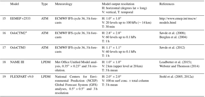
The transport of the radioactive cloud across the North-ern Hemisphere is illustrated in Fig. 2, as simulated by the FLEXPART model using meteorological analysis data from the Global Forecast System (GFS) model of the National Centers for Environmental Prediction (NCEP), in the weeks following the initial release at FD-NPP. While transport pat-terns depend on the meteorological data set used (e.g. some models generate their own meteorology), it can be seen that 3–4 weeks after the start of the emissions, the radionuclides
were already distributed fairly homogeneously over the en-tire Northern Hemisphere.
4 Methods
We use the same basic approaches as in Kristiansen et al. (2012) to evaluate measured and modelled loss of aerosol mass with time, i.e. aerosol lifetimes. Measured aerosol life-times, derived directly from the decay of station measure-ments of cesium (137Cs) and xenon (133Xe) (Kristiansen et al., 2012), are compared to modelled aerosol lifetimes deter-mined in exactly the same way from modelled station con-centrations for the same time periods as the observations. To reduce the variability caused by atmospheric transport, we normalize the137Cs values by the133Xe values; i.e. the ra-tio of the aerosol (137Cs) to the passive tracer (133Xe) is used throughout all lifetime evaluations. This largely compensates for variability in transport, but not completely because the source terms for137Cs and133Xe are not perfectly correlated. Additionally, we use global burdens estimated from measure-ment data as in Kristiansen et al. (2012) and compare these to modelled global burdens.
Several definitions of atmospheric lifetime exist. In Kris-tiansen et al. (2012), the e-folding lifetime was used as a measure of aerosol lifetime. Croft et al. (2014) docu-ment, compare, and explain differences between global mean aerosol lifetime, the definition typically reported for aerosol and climate model simulations, and e-folding times from their GEOS-Chem transport simulations of the FD-NPP ac-cident emissions. They show that the two definitions are not directly comparable for the FD-NPP case. The lifetime re-sults for the former definition were heavily influenced by
FD−NPP Wak Oah Yel Ash Char StJ Sch Spi Sto UlaUss 18 Mar 2011 12:00 UTC Latitude −20 0 20 40 60 80 FD−NPP Wak Oah Yel Ash Char StJ Sch Spi Sto UlaUss Latitude Longitude −100 0 100 −20 0 20 40 60 80 FD−NPP
Wak OahAsh Yel
Cha StJ SchSto Spi Ula Uss Altitude [km AGL] Latitude −200 0 20 40 60 80 5 10 15 20 FD−NPP Wak Oah Yel Ash Char StJ Sch Spi Sto UlaUss 25 Mar 2011 12:00 UTC FD−NPP Wak Oah Yel Ash Char StJ Sch Spi Sto UlaUss Longitude −100 0 100 FD−NPP
Wak OahAsh Yel
Cha StJ SchSto Spi Ula Uss Latitude −20 0 20 40 60 80 FD−NPP Wak Oah Yel Ash Char StJ Sch Spi Sto UlaUss 08 Apr 2011 12:00 UTC FD−NPP Wak Oah Yel Ash Char StJ Sch Spi Sto UlaUss Longitude −100 0 100 FD−NPP
Wak OahAsh Yel
Cha StJ SchSto Spi Ula Uss Latitude −20 0 20 40 60 80 FD−NPP Wak Oah Yel Ash Char StJ Sch Spi Sto UlaUss 21 Apr 2011 12:00 UTC Surface layer conc. [kBq m ] –3 1e−06 1e−05 1e−04 1e−03 1e−02 1e−01 1e−00 FD−NPP Wak Oah Yel Ash Char StJ Sch Spi Sto UlaUss Longitude −100 0 100 Total column [kBq m ] –2 1e−02 1e−01 1e−00 1e+01 1e+02 1e+03 1e+04 FD−NPP
Wak OahAsh Yel
Cha StJ SchSto Spi Ula Uss Latitude −20 0 20 40 60 80 Concentration [kBq m ] –3 1e−06 1e−05 1e−04 1e−03 1e−02 1e−01 1e−00
Figure 2. The transport of the radioactive plume of133Xe released from the Fukushima Dai-Ichi nuclear power plant (FD-NPP; black star) as simulated by the FLEXPART model using GFS meteorological data.133Xe surface concentrations (upper panel), total atmospheric columns (middle panel), and zonal mean vertical distribution (lower panel) for 18, 25 March, 8 and 22 April 2011 (1, 2, 4, and 6 weeks, respectively, after the start of the initial release on 11 March). The 11 CTBTO stations are marked with black points (please note that the points in the lower panel do not reflect the real station elevations).
initial quick removal, giving a much shorter lifetime than the e-folding lifetime for the hemispherically relatively well-mixed phase starting about 3 weeks after the main emissions. They also show that the global mean aerosol lifetime strongly depends on the altitude where emissions are assumed to oc-cur, while the e-folding lifetime is relatively insensitive to emissions parameters such as altitude, location, and time, suggesting that e-folding times allow a robust comparison between modelled and measurement-based lifetimes. For the purpose of this study we consider lifetime as equivalent to residence time.
In this exercise, we will use the e-folding lifetime (as in Kristiansen et al., 2012) and the instantaneous lifetime (as in Croft et al., 2014) as means of evaluation. The two life-times are typically used to evaluate exponentially decreasing aerosol concentrations after an emissions pulse.
The e-folding lifetime is defined as
τe= −ti
lnC(tC(ti)
0)
, (1)
where C(ti)is the concentration at time ti, C(t0)the initial concentration at time t0, and ti is the time since t0. Instanta-neous lifetime is defined as
τinst=
t(i−1)−ti
ln C(ti) C(ti−1)
, (2)
where ti and ti−1are adjacent time steps, here in this study separated by 1 day.
Further, we calculate the mean and median of all the mod-elled lifetimes. These are calculated from the lifetimes ob-tained for each model. Since the distribution of the modelled lifetime data is not symmetric but has outliers, the mean is not the best representative of the centre of the data, and there-fore the median is preferred. The variability is given as the standard deviation (SD) from the mean, and the median ab-solute deviation (MAD) from the median. The MAD is de-fined as the median of the absolute deviations from the data’s median:
where N is the total number of models and τi is the lifetime
(either e-folding or instantaneous) obtained from model i.
5 Results
5.1 Direct comparison of measured and modelled aerosol lifetimes
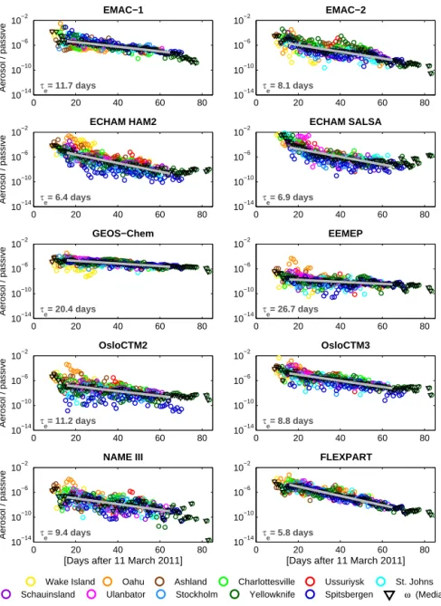
Here we present a direct comparison of measured and mod-elled aerosol lifetimes based on an observational constraint provided by radionuclide measurements of the FD-NPP emissions. We investigate the causes of differences between the measurements and models. The measured and modelled aerosol lifetimes are estimated from the ratios of the aerosol (137Cs) to the passive tracer (133Xe) surface concentrations (Sect. 4) at 11 CTBTO measurement sites (Sect. 3) as shown in Fig. 3. Both the measurements and all model simulations show a decrease in these ratios with time due to the removal of aerosols. The aerosol lifetimes are estimated by fitting an exponential decay model (grey lines in Fig. 3) to the daily median ratios over all stations (black triangles; ω in Fig. 3), between 15 and 65 days after the start of the emissions on 11 March. During this time period, measurement data ex-ist from at least five stations each day; i.e. the daily me-dian value ω is calculated from at least five values. The data density before day 15 and after day 65 is quite sparse and there are sampling biases. Before day 15, the measurements are mainly from the closest stations as the plume has not yet reached all sites and mixed through the Northern Hemi-sphere. After day 65, valid measurement data become sparse because concentrations start to drop below the detection limit and all data below the detection limit were discarded. The re-maining valid data after day 65 are mainly from Yellowknife and Spitsbergen with values near the detection limit. If these periods were considered, the lifetimes would be biased high, possibly due to a latitude effect, discussed later.
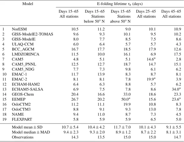
The measured aerosol (137Cs) to the passive tracer (133Xe) ratios decay with an e-folding lifetime τe(Eq. 1) of 14.3 days (Fig. 3 and Table 2) with a 95 % confidence interval of 13.1–15.7 days (Appendix B and Table B1). The equivalent modelled τelifetimes vary between 4.8 and 26.7 days with a model mean (±standard deviation) of 10.7 ± 5.5, and a model median (±MAD, Eq. 3) of 9.4 ± 2.3 days (Table 2). Thus, the model mean and median lifetimes are shorter than the lifetime based on the measurements, indicating too quick a removal of the aerosols in the models. However, some indi-vidual models have longer lifetimes than measured, and the model mean ±standard deviation encompasses the measured lifetime. Large variations in the modelled lifetimes are ex-pected due to differences in the simulated transport and es-pecially tropospheric removal.
Table 2 shows the lifetime estimates using data only from stations below and above 50◦N separately. Both mea-sured and mean modelled lifetimes are shorter below 50◦N
than at high latitudes, suggesting less efficient aerosol re-moval at high latitudes during the time period investigated (March–June). However, a few models (NorESM, ULAQ-CCM, EMAC-1, EMAC-2, and NAME) also have somewhat shorter lifetimes at higher latitudes than at lower latitudes, and two models (CAM5 and FLEXPART) show no change in lifetime with latitude. H. Wang et al. (2013) found that CAM5, with the shortest lifetimes of all models, overesti-mates aerosol wet removal by super-cooled liquid in mixed-phase clouds, which was improved in CAM5_PNNL. There is a larger spread in model lifetimes and larger deviations from the measurements at high latitudes compared to at lower latitudes, indicating larger uncertainties in the simulation of aerosols at higher latitudes. Similarly, lifetime estimates from the earlier phases (25–45 days after the start of the re-lease, a period when the major emissions were over) are com-pared to those for later time periods (days 45–65) (Table 2). Both the measurements and the median model give slightly longer lifetimes (by about 0.3–1.0 days) for the earlier phases than for later time periods. This is perhaps unexpected as the radionuclides are initially located in the lower troposphere where they are strongly affected by precipitation scaveng-ing and dry deposition, and later when the radionuclides are mostly located in the relatively dry upper troposphere (or even stratosphere), the removal processes are much less ef-fective which would yield an increase in lifetime. However, since the data used to derive the lifetimes are ground-based and thus biased towards that part of the aerosol population residing in the lower troposphere, neither the measurements nor the models may fully reflect the increase in lifetime due to transport in the upper troposphere. Differences in lifetime between tracers emitted near the surface and those coming from the stratosphere may be substantial, as discussed in Kristiansen et al. (2012). Furthermore, most of the radionu-clides were uplifted immediately after the release (Stohl et al., 2012a) and thus quite well mixed in the troposphere al-ready for the earlier time period (days 25–45), as also shown in Fig. 2. In addition, station data from the later time periods (day 45–65) include fewer data points in the calculations than in the earlier phases. Lastly, there are larger variations in the modelled lifetimes for the later phase, and a larger model to measurement deviation, indicating larger uncertainty in the modelled lifetimes for the later phase than for the earlier phase.
In summary, both the mean and median modelled aerosol lifetimes are somewhat shorter than the observed aerosol life-time, although they mostly agree within the standard devia-tions of the modelled lifetimes. The underestimation of life-times by the models is smaller than what was indicated by Kristiansen et al. (2012) based on reported mean modelled lifetimes from the literature, consistent with the findings of Croft et al. (2014). The deviations between observed and modelled aerosol lifetimes are largest for the northernmost stations and at later time periods, indicating higher
uncer-Table 2. E-folding aerosol lifetimes (Eq. 1) estimated from the decay of the ratios between the aerosol (137Cs) and the passive tracer (133Xe) surface concentrations at 11 station locations. Variations in lifetime for different latitude regions (below and above 50◦N) and time periods are also given. Mean and median modelled lifetimes are calculated from the lifetimes obtained for each model and the variability is given as standard deviation (SD) and median absolute deviation (MAD, Eq. 3). The data are shown in Fig. 3. 95 % confidence intervals and R2 statistics are given in Appendix B, Table B1. Values that are not statistically significant are marked with a star and were not considered for the mean and median calculations.
Model E-folding lifetime τe(days)
Days 15–65 Days 15–65 Days 15–65 Days 25–45 Days 45–65 All stations Stations Stations All stations All stations
below 50◦N above 50◦N 1 NorESM 10.5 11.2 9.0 10.1 10.9 2 GISS-ModelE2-TOMAS 9.6 9.3 10.1 9.5 10.2 3 GISS-ModelE 8.0 7.7 8.5 7.5 8.6 4 ULAQ-CCM 6.0 6.4 5.7 5.7 4.3 5 BCC_AGCM 16.7 17.7 18.5 17.9 12.6 6 LMDZORINCA 11.5 10.0 16.1 6.9 17.5 7 CAM5 4.8 5.1 5.1 14.6∗ 2.8 8 CAM5_PNNL 12.5 12.7 18.7 14.7 15.1 9 CAM5_NDG 7.7 7.3 9.8 6.1 6.2 10 EMAC-1 11.7 13.9 8.3 8.7 8.1 11 EMAC-2 8.1 8.1 7.8 19.9∗ 3.9 12 ECHAM-HAM2 6.4 6.3 8.8 5.7 6.2 13 ECHAM5-SALSA 6.9 7.5 7.8 8.6 34.0∗ 14 GEOS-Chem 20.4 16.6 33.0 18.6 23.3 15 EEMEP 26.7 20.2 50.0∗ 15.6 23.6∗ 16 OsloCTM2 11.2 11.1 19.9 10.8 8.3 17 OsloCTM3 8.8 9.1 9.3 13.0 7.8 18 NAME 9.4 11.0 8.7 7.3 4.5 19 FLEXPART 5.8 5.9 5.9 6.5 5.0 Model mean ± SD 10.7 ± 5.4 10.4 ± 4.2 11.7 ± 7.0 10.1 ± 4.3 9.1 ± 5.5 Model median ± MAD 9.4 ± 2.3 9.3 ± 2.0 8.9 ± 1.2 8.7 ± 2.2 8.1 ± 3.1
Observations 14.3 13.5 15.0 15.0 14.7
tainties in the simulation of aerosols and aerosol lifetimes at higher latitudes and later times.
5.2 Model evaluation of latitudinal variations in transport and scavenging
The previous section indicated that disagreements between the measurements and the models are largest at higher lati-tudes and at later time periods. This agrees with several pre-vious studies (e.g. Shindell et al., 2008; Koch et al., 2009), which suggest that models do not capture the Arctic aerosol variations very well. In this study, we have the possibility to evaluate the models’ abilities to simulate the aerosol concen-trations and transport at different latitudes, by comparing the measured and modelled aerosol (137Cs) and the passive trans-port tracer (133Xe) data. In this way, we can directly explore how well the models are able to reproduce the observations at the northernmost stations (i.e. above 60◦N; Yellowknife 62.5◦N and Spitsbergen 78◦N) compared to at lower lati-tudes. We also examine whether there are any temporal vari-ations in the model–observation devivari-ations. The analyses are
limited by the low number of Arctic/subarctic stations and the particular season and time period (March–June 2011) of the measurements. Some indications may still be given which might help explain shortcomings with simulated scavenging and/or transport in the models, and if one is the more likely cause for deviations to observations.
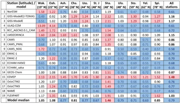
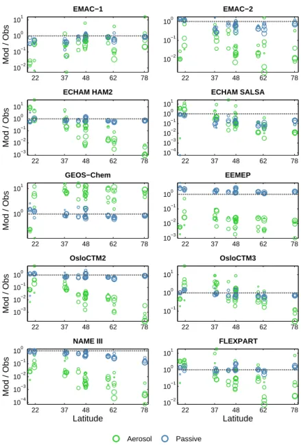
We use the ratio of the modelled to measured surface con-centrations as means of model score, where a ratio > 1 indi-cates that the model over-predicts, and a ratio < 1 represents under-predictions (Tables 3 and 4). Figure 4 shows the ra-tio of modelled to observed aerosol (green circles) and pas-sive transport tracer (blue circles) concentrations as a func-tion of latitude of the measurement stafunc-tions. Generally, the models reproduce the observed passive tracer (133Xe) values better than the observed aerosol (137Cs) values, indicating that transport is reasonably well represented in the models. Scavenging affects only the aerosols, causing more variabil-ity and a larger extent of over- or under-prediction. On aver-age, over all stations and models, the median ratio of mod-elled to measured passive tracer values is 0.79 (Table 3) and
0 20 40 60 80 10−14 10−10 10−6 10−2 τe= 14.3 days Aerosol / passive Measurements 0 20 40 60 80 10−14 10−10 10−6 10−2 τe= 10.5 days NorESM 0 20 40 60 80 10−14 10−10 10−6 10−2 τe= 9.6 days Aerosol / passive GISS−ModelE2−TOMAS 0 20 40 60 80 10−14 10−10 10−6 10−2 τe= 8.0 days GISS−ModelE 0 20 40 60 80 10−14 10−10 10−6 10−2 τe= 6.0 days Aerosol / passive ULAQ−CCM 0 20 40 60 80 10−14 10−10 10−6 10−2 τe= 16.7 days BCC AGCM, v.2.0.1 CAM 0 20 40 60 80 10−14 10−10 10−6 10−2 τe= 11.5 days Aerosol / passive LMDZORINCA 0 20 40 60 80 10−14 10−10 10−6 10−2 τe= 4.8 days CAM5, v5.1 0 20 40 60 80 10−14 10−10 10−6 10−2 τe= 12.5 days Aerosol / passive
[Days after 11 March 2011] CAM5, PNNL, v5.1 0 20 40 60 80 10−14 10−10 10−6 10−2 τe= 7.7 days
[Days after 11 March 2011] CAM5, NDG, v5.1
Wake Island Oahu Ashland Charlottesville Ussuriysk St. Johns Schauinsland Ulanbator Stockholm Yellowknife Spitsbergen ω (Median)
Figure 3.
for the aerosols 0.49 (Table 4), suggesting a general under-prediction of both aerosol and passive tracer concentrations. The aerosol underestimation is consistent with the lifetime results from the previous section (Sect. 5.1) which showed that modelled aerosol lifetimes are too short compared to the measurements, and this would yield too much removal and thus under-predictions of the aerosol concentrations.
Furthermore, at the southernmost stations (Wake Island and Oahu) many models over-predict both the aerosol and passive tracer concentrations, whilst under-predicting both at the stations further north (Tables 3 and 4). The exception is Schauinsland (48◦N) where the models generally over-predict the passive tracer but under-over-predict the aerosol val-ues. We find the largest under-prediction at the northernmost stations: Yellowknife for the passive tracer and Spitsbergen
for the aerosol values. The modelled to measured aerosol ratios have a pronounced latitudinal trend, with ratios de-creasing (i.e. larger under-predictions) with inde-creasing lati-tude (Table 4 and Fig. 4). This indicates that there is too much aerosol removal occurring en route to the Arctic. There is also a slight decrease in modelled to measured passive tracer ratios with latitude (Table 3 and Fig. 4), suggesting that trans-port to the high latitudes is also not strong enough in the mod-els, and this contributes to the aerosol underestimates at high latitudes. However, the main reason for the aerosol under-estimates at high latitudes must be too efficient a simulated removal.
Finally, Fig. 4 illustrates the temporal variations of mod-elled to measured ratios. The values are medians over 14 day time periods and the size of the circles indicates the time; the
0 20 40 60 80 10−14 10−10 10−6 10−2 τe= 11.7 days Aerosol / passive EMAC−1 0 20 40 60 80 10−14 10−10 10−6 10−2 τe= 8.1 days EMAC−2 0 20 40 60 80 10−14 10−10 10−6 10−2 τe= 6.4 days Aerosol / passive ECHAM HAM2 0 20 40 60 80 10−14 10−10 10−6 10−2 τe= 6.9 days ECHAM SALSA 0 20 40 60 80 10−14 10−10 10−6 10−2 τe= 20.4 days Aerosol / passive GEOS−Chem 0 20 40 60 80 10−14 10−10 10−6 10−2 τe= 26.7 days EEMEP 0 20 40 60 80 10−14 10−10 10−6 10−2 τe= 11.2 days Aerosol / passive OsloCTM2 0 20 40 60 80 10−14 10−10 10−6 10−2 τe= 8.8 days OsloCTM3 0 20 40 60 80 10−14 10−10 10−6 10−2 τe= 9.4 days Aerosol / passive
[Days after 11 March 2011] NAME III 0 20 40 60 80 10−14 10−10 10−6 10−2 τe= 5.8 days
[Days after 11 March 2011] FLEXPART
Wake Island Oahu Ashland Charlottesville Ussuriysk St. Johns Schauinsland Ulanbator Stockholm Yellowknife Spitsbergen ω (Median)
Figure 3. Time series of measured and modelled ratios of the aerosol (137Cs) to the passive tracer (133Xe) surface concentrations at 11 CTBTO station locations. ω values (median, black triangles) represent the daily median ratios (median concentration for each day over all stations). Fits of exponential decay models to the ω data are shown as grey lines with e-folding timescales τe(Eq. 1) as indicated. The fits
are made over days 15 to 65 for which data exist from at least five stations each day.
larger the circle, the later the time period. Particularly for the aerosol values, some models tend to show a stronger under-estimation with time, also evident in the median model.
Our results suggest that modelling of both scavenging and transport are causes for disagreements with observations. Transport to the high latitudes is not strong enough in the models, and this contributes to the model underestimates also of the aerosol tracer at high latitudes. However, the modelled to observed ratios decrease much more strongly with latitude for the aerosol than for the passive tracer, and this indicates that a problem with the aerosol scavenging is the major rea-son for disagreement between the simulations and the
mea-surements. Scavenging in the models depends strongly on the representation of clouds (temporal and spatial occurrence and dimensions) as well as on the amount of precipitation, which are likely to be the underlying issues. This helps ex-plain the larger deviations between measured and modelled aerosol lifetimes for the northernmost stations and at later time periods as seen in the previous section (Table 2).
5.3 Instantaneous lifetimes
The time variations in aerosol lifetimes can be examined fur-ther by considering the instantaneous lifetimes, τinst(defined
Table 3. Median ratio of the modelled to measured passive tracer (133Xe) surface concentrations, for each model and each station as well as the model median and over all stations. Values greater than 1.2 (substantial over-predictions) are shown in red, and values less than 0.8 (substantial under-predictions) in blue.
Table 4. Same as Table 3 but for aerosol (137Cs) surface concentrations.
in Sect. 4). In this section we use global modelled data as opposed to the previous sections that focused on modelled concentrations at the measurement stations. The estimate of instantaneous lifetimes uses the global aerosol (137Cs) and passive tracer (133Xe) burdens as simulated by the mod-els. Kristiansen et al. (2012) also provide an estimate for the burdens using the station measurements and a 1-D box
model. This estimate is however limited by the assumption of a well-mixed state in the atmosphere and only valid ap-proximately after about 3 weeks after the release until about 9 weeks (Appendix C). Therefore, global burdens estimated from the measurement data are only available for a limited time period. The global burdens are shown in Appendix C and Fig. C1. The modelled global aerosol (137Cs) burdens
22 37 48 62 78 100 101 NorESM 22 37 48 62 78 100 101 Mod / Obs GISS−ModelE2−TOMAS 22 37 48 62 78 10−1 100 101 GISS−ModelE 22 37 48 62 78 10−2 10−1 100 101 102 103 Mod / Obs ULAQ−CCM 22 37 48 62 78 100 101 BCC AGCM, v.2.0.1 CAM 22 37 48 62 78 10−2 10−1 100 Mod / Obs LMDZORINCA 22 37 48 62 78 10−5 10−4 10−3 10−2 10−1 100 CAM5, v5.1 22 37 48 62 78 100 101 Mod / Obs Latitude CAM5, PNNL, v5.1 22 37 48 62 78 10−1 100 101 Latitude CAM5, NDG, v5.1 22 37 48 62 78 10−1 100 Mod / Obs Model median Aerosol Passive Figure 4.
increase initially due to continuous cesium emissions but decrease as the aerosols are removed from the atmosphere, while the passive tracer (133Xe) global burdens stay approx-imately constant in the models after the xenon emissions cease. In the following, we analyse the instantaneous life-times obtained from the global burdens.
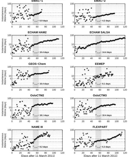
We use the ratios of the aerosol (137Cs) to the passive tracer (133Xe) global burdens, and calculate the instanta-neous lifetimes (Eq. 2) from these ratios, as shown in Ta-ble 5 and Fig. 5. In the first week after the start of the release, the modelled instantaneous lifetimes are about 2 days (Ta-ble 5), much shorter than the e-folding lifetimes presented in Sect. 5.1 for later time periods. This illustrates that the initial removal was quicker, as previously suggested by Kris-tiansen et al. (2012) and illustrated in Croft et al. (2014). This is due to the emissions occurring at low altitudes and
co-location of the plume with strong precipitation. After about 3 weeks, estimates for the instantaneous lifetimes from the measurement data are also possible and give a lifetime of 9.3–10.9 days, which is mostly longer than the median model lifetime of about 6.0–10.4 days (Table 5). After about 7 weeks (day 45–50), the instantaneous lifetimes reach some quasi-steady state with less variability (Fig. 5). The occur-rence of this less variable steady state is related to the emis-sions. Between day 10 and 40 there are low-level emissions of 137Cs, about 1 order of magnitude less than during the highest emissions around day 5. Because the emission was a point source (and not global) and its geographical distribu-tion is rather local, one continues to see the impact of single deposition events, making the instantaneous lifetime fluctu-ate considerably. On day 40 all emissions of137Cs end in the model simulations. The planetary boundary layer (PBL)
22 37 48 62 78 10−2 10−1 100 101 Mod / Obs EMAC−1 22 37 48 62 78 10−2 10−1 100 EMAC−2 22 37 48 62 78 10−3 10−2 10−1 100 101 Mod / Obs ECHAM HAM2 22 37 48 62 78 10−4 10−3 10−2 10−1 100 101 ECHAM SALSA 22 37 48 62 78 100 101 Mod / Obs GEOS−Chem 22 37 48 62 78 10−3 10−2 10−1 100 EEMEP 22 37 48 62 78 10−3 10−2 10−1 100 Mod / Obs OsloCTM2 22 37 48 62 78 10−1 100 101 OsloCTM3 22 37 48 62 78 10−4 10−3 10−2 10−1 100 Mod / Obs Latitude NAME III 22 37 48 62 78 10−2 10−1 100 101 Latitude FLEXPART Aerosol Passive
Figure 4. Ratio of modelled to observed aerosol (green) and passive tracer (blue) surface concentrations as a function of the latitude of the
measurement station and time; values at each measurement station are the median values over 14 day time periods (11–24 March, 25 March– 7 April, 8–21 April, 22 April–5 May, 6–19 May, 20 May–2 June, 3–17 June 2011). The size of the circles indicate the time; the larger the circle, the later the time period. Values above the dotted 1-line are over-predicted by the model and values below 1 are under-predictions. Notice different scales on the y axes.
is soon emptied of most 137Cs, and the remaining 137Cs (mainly in the free troposphere) is more widely spread and gives rise to a more stable instantaneous lifetime, and thus a quasi-steady state with less variability. The modelled in-stantaneous lifetimes over days 49 to 63 (weeks 8–9; shaded area in Fig. 5) vary between 2.8 and 19.0 days with a model median of 10.4 ± 2.5 days. The median instantaneous life-time for the same life-time period based on the measurements is 9.6 ± 0.7 days. In this period, the median modelled lifetimes are closer to, but slightly longer than those based on measure-ment data, in contrast to earlier phases. This could be due to more prominent modelled than real mixing into the
strato-sphere where lifetimes are longer. This stratospheric mixing is not evident in the surface measurement data.
The further steady increase in the instantaneous lifetimes in the later phases after about day 65 (Fig. 5) is attributed to transport and mixing into regions where the lifetimes are longer, such as the upper troposphere and the stratosphere. After some time, the troposphere is mainly cleaned by wet scavenging while aerosols that have been transported into the stratosphere remain, as the removal there is inefficient, especially for AM aerosols for which also gravitational set-tling is very slow. The total aerosol mass and the lifetimes are then dominated by the stratospheric loading, giving a
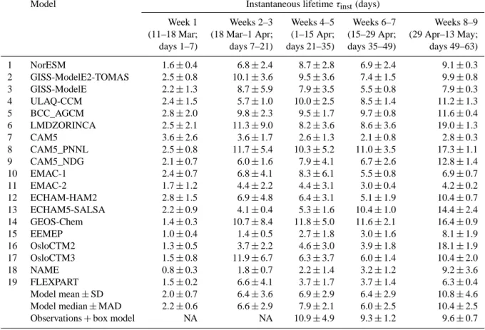
contin-Table 5. Median instantaneous lifetimes calculated from the ratios of the aerosol (137Cs) to the passive tracer (133Xe) global burdens during different time periods (weeks) after the start of the emissions (11 March 2011). The variability is given as the median absolute deviation (MAD, Eq. 3) for the individual models, as well as for the observations and the model median, while the standard deviation (SD) is given of the model mean. These variabilities are calculated from the instantaneous lifetimes over each of the time periods. The data are shown in Fig. 5.
Model Instantaneous lifetime τinst(days)
Week 1 Weeks 2–3 Weeks 4–5 Weeks 6–7 Weeks 8–9
(11–18 Mar; (18 Mar–1 Apr; (1–15 Apr; (15–29 Apr; (29 Apr–13 May; days 1–7) days 7–21) days 21–35) days 35–49) days 49–63)
1 NorESM 1.6 ± 0.4 6.8 ± 2.4 8.7 ± 2.8 6.9 ± 2.4 9.1 ± 0.3 2 GISS-ModelE2-TOMAS 2.5 ± 0.8 10.1 ± 3.6 9.5 ± 3.6 7.4 ± 1.5 9.9 ± 0.8 3 GISS-ModelE 2.2 ± 1.3 8.7 ± 5.9 7.9 ± 3.5 5.5 ± 0.8 7.9 ± 0.3 4 ULAQ-CCM 2.4 ± 1.5 5.7 ± 1.0 10.0 ± 2.5 8.5 ± 1.4 11.2 ± 1.3 5 BCC_AGCM 2.8 ± 2.0 9.8 ± 2.3 9.5 ± 1.7 9.7 ± 0.8 11.6 ± 0.4 6 LMDZORINCA 2.5 ± 2.1 11.3 ± 9.0 8.2 ± 3.6 8.6 ± 3.6 19.0 ± 1.3 7 CAM5 3.6 ± 2.6 3.6 ± 1.7 2.6 ± 1.3 2.1 ± 0.8 2.8 ± 0.3 8 CAM5_PNNL 2.5 ± 0.8 11.7 ± 5.4 10.3 ± 5.2 11.0 ± 3.5 17.3 ± 1.1 9 CAM5_NDG 2.1 ± 0.7 6.0 ± 1.6 7.9 ± 4.1 6.7 ± 2.6 12.8 ± 1.4 10 EMAC-1 2.4 ± 0.7 6.8 ± 4.1 8.3 ± 6.1 5.5 ± 0.8 6.9 ± 0.7 11 EMAC-2 1.7 ± 1.2 4.4 ± 2.2 4.4 ± 3.1 3.0 ± 0.4 4.2 ± 0.2 12 ECHAM-HAM2 2.8 ± 1.5 6.9 ± 4.8 6.4 ± 3.1 5.1 ± 1.9 10.4 ± 0.7 13 ECHAM5-SALSA 2.2 ± 0.9 4.1 ± 0.4 5.3 ± 1.6 10.4 ± 1.0 14.4 ± 2.4 14 GEOS-Chem 1.4 ± 0.3 10.7 ± 8.4 11.8 ± 5.0 11.6 ± 2.1 16.4 ± 0.9 15 EEMEP 1.0 ± 0.4 1.4 ± 0.5 2.7 ± 1.8 3.0 ± 1.6 8.1 ± 1.9 16 OsloCTM2 1.3 ± 0.5 3.7 ± 2.2 4.6 ± 3.0 3.9 ± 1.8 18.1 ± 1.9 17 OsloCTM3 1.5 ± 0.8 11.9 ± 6.7 6.3 ± 3.7 6.0 ± 1.4 10.4 ± 2.0 18 NAME 0.8 ± 0.3 1.8 ± 0.7 2.2 ± 1.4 3.2 ± 1.2 9.2 ± 3.6 19 FLEXPART 1.5 ± 0.2 6.6 ± 4.1 3.7 ± 1.7 3.7 ± 1.4 6.3 ± 0.4 Model mean ± SD 2.0 ± 0.7 6.4 ± 3.6 6.9 ± 2.9 6.4 ± 2.9 10.8 ± 4.6
Model median ± MAD 2.2 ± 0.6 6.6 ± 2.9 7.9 ± 2.1 6.0 ± 2.5 10.4 ± 2.5
Observations + box model NA NA 10.9 ± 4.9 9.3 ± 1.2 9.6 ± 0.7
uous increase in lifetime (Cassiani et al., 2013). The large variations in the steady increase of instantaneous lifetime be-tween models might be related to how the models simulate transport into the upper troposphere and stratosphere. The longest lifetimes at later stages are probably given by models that inject a fraction of the aerosols quickly into the strato-sphere (probably even by a single event) and have an effi-cient removal in the troposphere, which would give a large (and increasing) fraction of the aerosols residing in the up-per troposphere and stratosphere. Furthermore, models with diffusive advection schemes may excessively “leak” aerosols into the stratosphere. Thus, the instantaneous lifetimes at later stages are probably more indicative of the upper tropo-spheric/stratospheric aerosol fraction and are less useful to constrain tropospheric removal. In addition, the well-mixed assumption required for the measurement-derived lifetimes breaks down once a substantial fraction of the material is in the stratosphere. This means that measurement-derived and model-derived instantaneous lifetimes for the later phases are not entirely comparable, as they are not derived in a con-sistent way. It is expected that the measurement-derived in-stantaneous lifetimes are systematically lower, since they are
based on surface measurements with the assumption of a constant scale height. Calculating the global burdens based on the modelled station data and the box model reveals that for some models, the box-model estimates indeed underesti-mate the full global burdens (see Appendix C and Fig. C1).
In summary, we find that the modelled instantaneous life-times were initially short (about 1–2 days) and the initial removal quicker than for later time periods. At later times (weeks 4–7) the instantaneous lifetimes obtained by mea-surements were generally longer than obtained from the models, as also seen in Sect. 5.1 from station locations. After that, the modelled instantaneous lifetimes are influenced by mixing into the stratosphere and not representative anymore of scavenging processes in the troposphere.
6 Discussion
6.1 Interpretation of the aerosol lifetime estimates
To interpret our estimates of aerosol lifetime, we first dis-cuss an exemplified evolution of the aerosol burden after a
τinst = 9.6 days Instantaneous lifetime [days]
Measurements + box model
0 20 40 60 80 100 120 1 5 10 100 τinst = 9.1 days NorESM 0 20 40 60 80 100 120 1 5 10 100 τinst = 9.9 days
Instantaneous lifetime [days]
GISS−ModelE2−TOMAS 0 20 40 60 80 100 120 1 5 10 100 τinst = 7.9 days GISS−ModelE 0 20 40 60 80 100 120 1 5 10 100 τinst = 11.2 days
Instantaneous lifetime [days]
ULAQ−CCM 0 20 40 60 80 100 120 1 5 10 100 τinst = 11.6 days BCC AGCM, v.2.0.1 CAM 0 20 40 60 80 100 120 1 5 10 100 τinst = 19.0 days
Instantaneous lifetime [days]
LMDZORINCA 0 20 40 60 80 100 120 1 5 10 100 τinst = 2.8 days CAM5, v5.1 0 20 40 60 80 100 120 1 5 10 100 τinst = 17.3 days
Instantaneous lifetime [days]
[Days after 11 March 2011] CAM5, PNNL, v5.1 0 20 40 60 80 100 120 1 5 10 100 τinst = 12.8 days
[Days after 11 March 2011] CAM5, NDG, v5.1 0 20 40 60 80 100 120 1 5 10 100 Figure 5.
unit pulse emission (Fig. 6). In our example, the decay of the burden is not perfectly exponential but consists of differ-ent characteristic timescales. There is a fast initial removal with a short time decay τ1, which represents the time pe-riod when the aerosols are mostly residing in the PBL and are very susceptible to dry and wet deposition. The second period has slower removal with a timescale τ2, and repre-sents the period when most of the aerosols are residing in the free troposphere. The last time period, with the slowest de-cay timescale τ3, is the period when most of the aerosols are removed from the troposphere and only the fraction that was transported into the stratosphere remains.
The exemplified curve would depend on where on the globe the emissions take place, during which season, and it might differ from year to year. Thus, the timescales will
vary greatly for different cases, and also for different models simulating the meteorology for the given case differently. τ1 would be very different for all cases, probably depending on a few precipitation events, while different cases and models would have a smaller spread for τ2and τ3which are affected by processes on a more global scale. Global mean lifetimes (e.g. Croft et al., 2014) would be mainly determined by the initial behaviour (τ1)and it could be argued that knowing the initial lifetime is important for estimating the aerosol burden, the radiative forcing, and climate sensitivity.
In this study we focus mainly on the intermediate timescale τ2because sufficient measurement data were only available from about 2 weeks after the start of the release, un-til about day 65 (Sect. 5.1). We do not have sufficient mea-surements to constrain τ1, but it is likely that some of the
τinst = 6.9 days Instantaneous lifetime [days]
EMAC−1 0 20 40 60 80 100 120 1 5 10 100 τinst = 4.2 days EMAC−2 0 20 40 60 80 100 120 1 5 10 100 τinst = 10.4 days
Instantaneous lifetime [days]
ECHAM HAM2 0 20 40 60 80 100 120 1 5 10 100 τinst = 14.4 days ECHAM SALSA 0 20 40 60 80 100 120 1 5 10 100 τinst = 16.4 days
Instantaneous lifetime [days]
GEOS−Chem 0 20 40 60 80 100 120 1 5 10 100 τinst = 8.1 days EEMEP 0 20 40 60 80 100 120 1 5 10 100 τinst = 18.1 days
Instantaneous lifetime [days]
OsloCTM2 0 20 40 60 80 100 120 1 5 10 100 τinst = 10.4 days OsloCTM3 0 20 40 60 80 100 120 1 5 10 100 τinst = 9.2 days
Instantaneous lifetime [days]
[Days after 11 March 2011] NAME III 0 20 40 60 80 100 120 1 5 10 100 τinst = 6.3 days
[Days after 11 March 2011] FLEXPART 0 20 40 60 80 100 120 1 5 10 100
Figure 5. Instantaneous lifetimes calculated from the ratios of the aerosol (137Cs) to the passive tracer (133Xe) global burdens. The median instantaneous lifetimes τinstover days 49–63 (weeks 8–9; 29 April–13 May; shaded area) are indicated, and represent the time period when
the ratios have reached a quasi-steady state, and influence from transport into the stratosphere is less significant than for later times. The measurement + box model refers to the estimate from Kristiansen et al. (2012) for the burdens using the station measurements and a 1-D box model (see Appendix C and Fig. C1).
same processes contribute to the determination of both τ1and τ2. While τ1is probably mainly impacted by processes within the PBL, τ2is additionally influenced by how the aerosols are mixed out of the PBL, transported in the free troposphere, and finally brought back into the PBL. That way it is possi-ble that models that capture τ2well also perform well for τ1. In our case, another difference between τ1and τ2is that the former was mostly determined by a few individual precipita-tion events near Fukushima, while the latter is determined by removal occurring worldwide.
The evolution of the burden in Fig. 6 can be approximated by the sum of three exponential functions, i.e.
f (t ) = f1exp −t τ1 +f2exp −t τ2 +f3exp −t τ3 , (4) where f1+f2+f3=1.
A mean lifetime can be calculated as
τm=f1τ1+f2τ2+f3τ3, (5)
which corresponds to the area under the curve f (t ).
Using an optimizing convolution approach we can find the coefficients in Eq. (4) which give the best agreement
be-20 40 60 1.0 10.0 τ1 τ 2 τ 3 Burden Time
Figure 6. Exemplified evolution of the aerosol burden after a unit
emission, with characteristic timescales indicated by τ1, τ2, and τ3.
tween the aerosol burdens obtained from the model simu-lations (Appendix C) and the expression in Eq. (4). Table 6 shows the characteristic timescales τ1, τ2, and τ3 obtained from the convolution approach, calculated for the different models from their aerosol (137Cs) burdens, as well as the mean lifetime τm(Eq. 5). The initial timescale τ1is fastest and around 2 days, which is related to the low-altitude emis-sions of hydrophilic aerosols. The intermediate timescale τ2 is around 12 days, and the longest timescale τ3about 150– 200 days. The estimated τ3is very uncertain for most mod-els as it is very close to the a priori estimate of 200 days. The exceptions are the NorESM and GISS-ModelE models which had longer time series available. The model mean and median for τ3 are therefore calculated based on these two models only. The mean lifetime τmis rather short, on the or-der of 2–3 days, and is strongly affected by τ1, which was also demonstrated by Croft et al. (2014). The estimate for τ2 shows good agreement with the instantaneous lifetime τinst over weeks 8–9 from Fig. 5 and Table 5, and for most mod-els the e-folding lifetime τefrom Fig. 3 and Table 2 also fits well with τ2. This clearly demonstrates that in this study the focus is on the intermediate timescale τ2.
6.2 Causes of model–observation deviations and model differences
Our results show that there are significant deviations be-tween aerosol lifetimes obtained from models and those ob-tained from observations. The modelled lifetimes have a large spread but are generally shorter than the observed life-time. In addition, large biases in model to observed surface concentrations were found, with an overall under-prediction of both the aerosol (137Cs) and passive tracer (133Xe) concen-trations. The model–observation deviations can be due to in-accuracies in the source emissions, errors in scavenging and convective transport, and incorrect diffusivity of the models. These issues are discussed more in the following.
Inaccuracies in the source emissions will affect the abso-lute model-simulated values and therefore the biases in the
model to observed concentrations (Tables 3–4 and Fig. 4). It cannot be ruled out that our137Cs emissions are too low, or there were errors in the injection heights. However, the 137Cs source term used is rather on the high side compared to others (e.g. Chino et al., 2011). Also, the133Xe source term has been confirmed independently (Stohl et al., 2012b) and has rather low uncertainty. Overall, uncertainties in the as-sumed source term and its implementation are likely not the main reasons for the general underestimation of the aerosol (137Cs) and passive tracer (133Xe) concentrations. The life-time estimates (Fig. 3 and Table 2) are not affected by the absolute values of the source term used. However, these life-time estimates would be affected by possible late emissions of radionuclides long after the start of the release. Such late additional releases could be either direct late emissions from FD-NPP or indirect releases by resuspension of deposited ra-dionuclides. Kristiansen et al. (2012) discussed this uncer-tainty and found no evidence for such late emissions, neither in the measurement data nor in the existing literature on the FD-NPP accident.
Most models have treated cesium solely as sulfate aerosols, while it is possible that some of the cesium attached to other aerosol components with different deposition prop-erties. Initially, many non-soluble aerosols could have been present around the power plant, which might be removed less efficiently from the atmosphere in the first days after emis-sion before mixing internally with soluble aerosol compo-nents. The assumption that cesium attached solely to sulfate could result in scavenging that is too strong during the first few days after the release, and can therefore contribute to the overall underestimations of the aerosol (137Cs) concentra-tions (Table 4). The e-folding lifetimes (Table 2) should not be affected by errors in the modelled scavenging efficiency in the initial phase (τ1 in Fig. 6), as the e-folding lifetimes have been derived only for later periods (after 15 days, i.e. τ2 in Fig. 6) when the aerosols are likely internally mixed and aerosol components undergo similar removal.
More importantly, the models’ treatment of aerosol scav-enging is essential for both the modelled lifetime and ab-solute concentrations. The modelled representation and dis-tribution of clouds, as well as rain patterns and rain inten-sity, are important factors since they determine where and how much aerosol is removed. Further, the horizontal resolu-tion of the model and meteorological input data might have a large impact in terms of clouds and precipitation (inten-sity and spatial extent). Higher horizontal resolution can in general lead to more resolved large-scale and less sub-grid convective clouds (Hagemann et al., 2006). The scavenging parameterizations, including cloud and rain definitions and occurrences, differ greatly between the models (Table A1), and are likely the major cause of model differences and devi-ations between models and observdevi-ations. This issue is further discussed in Sect. 6.6.
Additionally, the coupling between aerosol scavenging and the convection scheme in the models may represent