HAL Id: hal-02104411
https://hal.archives-ouvertes.fr/hal-02104411
Submitted on 15 May 2019
HAL is a multi-disciplinary open access
archive for the deposit and dissemination of
sci-entific research documents, whether they are
pub-lished or not. The documents may come from
teaching and research institutions in France or
abroad, or from public or private research centers.
L’archive ouverte pluridisciplinaire HAL, est
destinée au dépôt et à la diffusion de documents
scientifiques de niveau recherche, publiés ou non,
émanant des établissements d’enseignement et de
recherche français ou étrangers, des laboratoires
publics ou privés.
a multi-scale tracer for carbon and water cycles
Mary Whelan, Sinikka Lennartz, Teresa Gimeno, Richard Wehr, Georg
Wohlfahrt, Yuting Wang, Linda Kooijmans, Timothy Hilton, Sauveur Belviso,
Philippe Peylin, et al.
To cite this version:
Mary Whelan, Sinikka Lennartz, Teresa Gimeno, Richard Wehr, Georg Wohlfahrt, et al.. Reviews
and syntheses: Carbonyl sulfide as a multi-scale tracer for carbon and water cycles. Biogeosciences,
European Geosciences Union, 2018, 15 (12), pp.3625-3657. �10.5194/bg-15-3625-2018�. �hal-02104411�
https://doi.org/10.5194/bg-15-3625-2018 © Author(s) 2018. This work is distributed under the Creative Commons Attribution 4.0 License.
Reviews and syntheses: Carbonyl sulfide as a multi-scale
tracer for carbon and water cycles
Mary E. Whelan1,2, Sinikka T. Lennartz3, Teresa E. Gimeno4, Richard Wehr5, Georg Wohlfahrt6, Yuting Wang7, Linda M. J. Kooijmans8, Timothy W. Hilton9, Sauveur Belviso10, Philippe Peylin10, Róisín Commane11, Wu Sun2, Huilin Chen8, Le Kuai12, Ivan Mammarella13, Kadmiel Maseyk14, Max Berkelhammer15, King-Fai Li16, Dan Yakir17, Andrew Zumkehr18, Yoko Katayama19, Jérôme Ogée4, Felix M. Spielmann6, Florian Kitz6, Bharat Rastogi20,
Jürgen Kesselmeier21, Julia Marshall22, Kukka-Maaria Erkkilä13, Lisa Wingate4, Laura K. Meredith23, Wei He8, Rüdiger Bunk21, Thomas Launois4, Timo Vesala13,24,25, Johan A. Schmidt26, Cédric G. Fichot27, Ulli Seibt2, Scott Saleska5, Eric S. Saltzman28, Stephen A. Montzka29, Joseph A. Berry1, and J. Elliott Campbell9
1Carnegie Institution for Science, 260 Panama St., Stanford, CA 94305, USA
2Department of Atmospheric and Oceanic Sciences, University of California, Los Angeles, 405 Hilgard Ave.,
7127 Math Sciences Building, Los Angeles, CA 90095-1565, USA
3GEOMAR Helmholtz-Centre for Ocean Research Kiel, Duesternbrooker Weg 20, 24105 Kiel, Germany 4INRA, UMR ISPA, 71 Avenue Edouard Bourleaux, 33140, Villenave d’Ornon, France
5Department of Ecology and Evolutionary Biology, University of Arizona, 1041 E. Lowell St., Tucson, AZ 85721, USA 6Institute of Ecology, University of Innsbruck, Sternwartestr. 15, 6020 Innsbruck, Austria
7Institute of Environmental Physics, University of Bremen, Otto-Hahn-Allee 1, 28359 Bremen, Germany 8Centre for Isotope Research, University of Groningen, Nijenborgh 6, 9747 AG Groningen, the Netherlands 9Environmental Studies Department, UC Santa Cruz, 1156 High St., Santa Cruz, CA 95064, USA
10Laboratoire des Sciences du Climat et de l’Environnement, CEA-CNRS-UVSQ-Paris Saclay,
Orme des Merisiers, 91191 Gif-sur-Yvette, France
11Harvard School of Engineering and Applied Sciences, 20 Oxford Street, Cambridge, MA 02138, USA
12UCLA Joint Institute for Regional Earth System Science and Engineering (JIFRESSE), Jet Propulsion Laboratory,
Caltech, 4800 Oak Groove Dr., M/S 233-200, Pasadena, CA 91109, USA
13Institute for Atmospheric and Earth System Research/Physics, Faculty of Science,
University of Helsinki, P.O. Box 68, 00014, Helsinki, Finland
14School of Environment, Earth and Ecosystem Sciences, The Open University, Walton Hall, Milton Keynes, UK 15Department of Earth and Environmental Sciences, University of Illinois at Chicago, Chicago, IL 60607, USA 16Environmental Sciences, University of California, Riverside, 900 University Ave,
Geology 2460, Riverside, CA 92521, USA
17Earth and Planetary Sciences, Weizmann Instiutute of Science, 234 Herzl St., Rehovot 76100, Israel 18University of California, Merced, 5200 N. Lake Rd., Merced, CA 95343, USA
19Center for Conservation Science, Tokyo National Research Institute for Cultural Properties,
3–43 Ueno Park, Taito-ku, 110–8713 Tokyo, Japan
20Forest Ecosystems and Society, Oregon State University, 374 Richardson Hall, Corvallis, OR 97333, USA 21Department of Multiphase Chemistry, Max Planck Institute for Chemistry, P.O. Box 3060, 55020 Mainz, Germany 22Max Planck Institute for Biogeochemistry, Hans-Knöll-Str. 10, 7745 Jena, Germany
23School of Natural Resources and the Environment, University of Arizona, 1064 E. Lowell St., Tucson, AZ 85721, USA 24Institute for Atmospheric and Earth System Research/Forest Sciences, Faculty of Agriculture and Forestry,
University of Helsinki, P.O. Box 68, 00014, Helsinki, Finland
25Viikki Plant Science Centre, University of Helsinki, 00014, Helsinki, Finland
26Department of Chemistry, University of Copenhagen, Universitetsparken, 2100 Copenhagen, Denmark
27Department of Earth and Environment, Boston University, 675 Commonwealth Avenue, Boston, MA 02215, USA 28Department of Earth System Science, University of California, Irvine, Croul Hall, Irvine, CA 92697-3100, USA
29NOAA/ESRL/GMD, 325 Broadway, Boulder, CO 80305, USA
Correspondence: Mary E. Whelan (mary.whelan@gmail.com)
Received: 13 October 2017 – Discussion started: 24 October 2017
Revised: 15 May 2018 – Accepted: 22 May 2018 – Published: 18 June 2018
Abstract. For the past decade, observations of carbonyl sul-fide (OCS or COS) have been investigated as a proxy for car-bon uptake by plants. OCS is destroyed by enzymes that in-teract with CO2during photosynthesis, namely carbonic
an-hydrase (CA) and RuBisCO, where CA is the more important one. The majority of sources of OCS to the atmosphere are geographically separated from this large plant sink, whereas the sources and sinks of CO2are co-located in ecosystems.
The drawdown of OCS can therefore be related to the uptake of CO2without the added complication of co-located
emis-sions comparable in magnitude. Here we review the state of our understanding of the global OCS cycle and its applica-tions to ecosystem carbon cycle science. OCS uptake is cor-related well to plant carbon uptake, especially at the regional scale. OCS can be used in conjunction with other indepen-dent measures of ecosystem function, like solar-induced flu-orescence and carbon and water isotope studies. More work needs to be done to generate global coverage for OCS ob-servations and to link this powerful atmospheric tracer to systems where fundamental questions concerning the carbon and water cycle remain.
1 Introduction
Carbonyl sulfide (OCS or COS, hereafter OCS) observations have emerged as a tool for understanding terrestrial carbon uptake and plant physiology. Some of the enzymes involved in photosynthesis by leaves also efficiently destroy OCS, so that leaves consume OCS whenever they are assimilat-ing CO2(Protoschill-Krebs and Kesselmeier, 1992; Schenk
et al., 2004; Notni et al., 2007). The two molecules diffuse from the atmosphere to the enzymes along a shared pathway, and the rates of OCS and CO2uptake tend to be closely
re-lated (Seibt et al., 2010). Plants do not produce OCS, and consumption in plant leaves is straightforward to observe. In contrast, CO2uptake is difficult to measure by itself. At
ecosystem, regional, and global scales, large respiratory CO2
fluxes from other plant tissues and other organisms obscure the photosynthetic CO2signal, i.e., gross primary
productiv-ity (GPP). OCS is not a perfect tracer for GPP due to the pres-ence of additional sources/sinks of OCS in ecosystems that complicate this relationship. However, these sources/sinks are generally small, so measurements of OCS concentrations and fluxes can still generate useful estimates of
photosynthe-sis, stomatal conductance, or other leaf parameters at tempo-ral and spatial scales that are difficult to observe.
Several independent groups have examined OCS and CO2
observations and come to similar conclusions about links be-tween the plant uptake processes for the two gases. Goldan et al. (1987) linked OCS plant uptake, FOCS, to uptake of
CO2, FCO2, specifically referring to GPP. Advancing the
global perspective, Chin and Davis (1993) thought FOCSwas
connected to net primary productivity, which includes res-piration terms, and this scaling was used in earlier versions of the OCS budget, e.g., Kettle et al. (2002). Sandoval-Soto et al. (2005) re-introduced GPP as the link to FOCS, using
available GPP estimates to improve OCS and sulfur budgets, which were their prime interest. Montzka et al. (2007) first proposed to reverse the perspective in the literature and sug-gested that OCS might be able to supply constraints on gross CO2fluxes, with Campbell et al. (2008) directly applying it
in this way.
Since then, other applications have been developed, in-cluding understanding of terrestrial plant productivity since the last ice age (Campbell et al., 2017a), estimating canopy (Yang et al., 2018) and stomatal conductance and enzyme concentrations on the ecosystem scale (Wehr et al., 2017), assessment of the current generation of continental-scale carbon models (e.g., Hilton et al., 2017), and better trac-ing of large-scale atmospheric processes like convection and tropospheric–stratospheric mass transfers. Many of these ap-plications rely on the fact that the largest fluxes of atmo-spheric OCS are geographically separated: most atmoatmo-spheric OCS is generated in surface oceans and is destroyed by ter-restrial plants. In practice, these new applications often call for refining the terms of the global budget of OCS.
An abundance of new observations have been made pos-sible by technological innovation. While OCS is the longest-lived and most plentiful sulfur-containing gas in the atmo-sphere, its low ambient concentration (∼ 0.5 ppb) makes measurement challenging. Quantification of OCS in air used to require time-consuming pre-concentration before injec-tion into a gas chromatograph (GC) with a mass spectrom-eter (MS) or other detector. While extended time series re-main scarce, 17 years of observations have been generated by the National Oceanic and Atmospheric Administration (NOAA) Global Monitoring Division air monitoring network (Montzka et al., 2007). A system for measuring flask sam-ples for a range of important low-concentration trace gases was modified slightly in early 2000 to enable reliable
mea-surements for OCS. These observations allowed for the first robust evidence of OCS as a tracer for terrestrial CO2
up-take on continental to global scales (Campbell et al., 2008). In 2009, a quantum cascade laser instrument was developed, followed by many improvements in precision and measure-ment frequency (Stimler et al., 2010a). Current instrumeasure-ments can measure OCS with < 0.010 ppb precision and a fre-quency of 10 Hz (Kooijmans et al., 2016). On larger spatial scales, many Fourier transform infrared spectroscopy (FTIR) stations and three satellites have recently been used to re-trieve spectral signals for OCS in the atmosphere.
This review seeks to synthesize our collective understand-ing of atmospheric OCS, highlight the new questions that these data help answer, and identify the outstanding knowl-edge gaps to address moving forward. First, we present what information is known from surface-level studies. Then we develop a scaled-up global OCS budget that suggests where there are considerable uncertainties in the flux of OCS to the atmosphere. We examine how the existing data have been applied to estimating GPP and other ecosystem variables. Fi-nally, we describe where data are available and prioritize top-ics for further research.
2 Global atmospheric OCS budget
The sulfur cycle is arguably the most perturbed element cycle on Earth. Half of sulfur inputs to the atmosphere come from anthropogenic activity (Rice et al., 1981). OCS is the most abundant and longest-lived sulfur-containing gas. Ambient concentrations of OCS are relatively stable over month-long timescales. Observations from flask (Montzka et al., 2007), FTIR (Toon et al., 2018), and Fourier transform spectroscopy (FTS) measurements (Kremser et al., 2015) suggest a small (< 5 %) increasing trend in tropospheric OCS for the most recent decade. Over millennia, concentrations may reflect large-scale changes in global plant cover (Aydin et al., 2016; Campbell et al., 2017a).
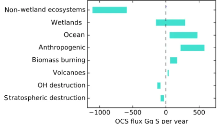
Upscaling ecosystem estimates (Sandoval-Soto et al., 2005) with global transport models are incompatible with atmospheric measurements (Berry et al., 2013; Sunthar-alingam et al., 2008), suggesting that there may be a large missing source of OCS, sometimes attributed to the tropical oceans; however, individual observations from ocean vessels do not necessarily support this hypothesis (Lennartz et al., 2017). The small increase of OCS in the atmosphere is at least 2 orders of magnitude too small to account for the miss-ing source. Anthropogenic emissions are an important OCS source to the atmosphere, but data for the relevant global in-dustries are incomplete (Zumkehr et al., 2018). Here we ana-lyze our current understanding of global surface–atmosphere OCS exchange and generate new global flux estimates from the bottom up, with no attempt at balancing the atmospheric budget (Fig. 1). We use the convention that positive flux
rep- Non-Wetlands Ocean A B V S
Figure 1. A bottom-up budget of atmospheric OCS on the global scale. Positive values indicate a source to the atmosphere. No at-tempt has been made to preserve mass balance. The contribution of lakes and non-vascular plants is included in the non-wetland ecosys-tem estimate. The small increase of OCS in the atmosphere is not included in this plot.
resents emission to the atmosphere and negative flux repre-sents removal.
2.1 Global atmosphere
OCS in the atmosphere is primarily generated from ocean and anthropogenic sources. A portion of these sources are in-direct, emitted as CS2which can be oxidized to OCS (Zeng
et al., 2016). Within the atmosphere, major sinks of OCS are OH oxidation in the troposphere and photolysis in the stratosphere. Besides large volcanic eruptions, OCS is a sig-nificant source of sulfur to the stratosphere and was briefly entertained as a geoengineering approach to promote global dimming (Crutzen, 2006). However, the global warming po-tential of OCS roughly balances whatever global cooling ef-fect it might have (Brühl et al., 2012). Abiotic hydrolysis in the atmosphere plays a small role: while snow and rain were observed to be supersaturated with OCS (Belviso et al., 1989; Mu et al., 2004), even in the densest supersaturated clouds the OCS in the air would represent 99.99 % of the OCS present (Campbell et al., 2017b). Multiple lines of evidence support uptake by plants as the dominant removal mecha-nism of atmospheric OCS (e.g., Asaf et al., 2013; Berry et al., 2013; Billesbach et al., 2014; Campbell et al., 2008; Glatthor et al., 2017; Hilton et al., 2017; Launois et al., 2015b; Mi-halopoulos et al., 1989; Montkza et al., 2007; Protoschill-Krebs and Kesselemeier, 1992; Sandoval-Soto et al., 2005; Stimler, 2010b; Suntharalingham et al., 2008).
The observed atmospheric OCS distribution suggests that seasonality is driven by terrestrial uptake in the Northern Hemisphere and oceanic fluxes in the Southern Hemisphere (Montzka et al., 2007). Improvements in the OCS budget were derived through inverse modeling of NOAA tower and airborne observations on a global scale (Berry et al., 2013; Launois et al., 2015b; Suntharalingam et al., 2008). Lower
concentrations were generally found in the terrestrial atmo-spheric boundary layer compared to the free troposphere dur-ing the growdur-ing season, and amplitudes of seasonal variabil-ity were enhanced at low-altitude stations, particularly those situated mid-continent.
Total column measurements of OCS from ground-based FTS show trends in OCS concentrations coincident with the rise and fall of global rayon production, which cre-ates OCS indirectly (Campbell et al., 2015). Kremser et al. (2015) found an overall positive tropospheric rise of 0.43–0.73 % yr−1 at three sites in the Southern Hemisphere from 2001 to 2014. The trend was interrupted by a sharply decreasing interval from 2008 to 2010, also observed in the global surface flask measurements (Fig. S2; Campbell et al., 2017a). A similar but smaller dip was observed in the stratosphere, indicating that the trends are driven by pro-cesses within the troposphere. Over Jungfraujoch, Switzer-land, Lejeune et al. (2017) observed a decrease in tropo-spheric OCS from 1995 to 2002 and an increase from 2002 to 2008; after 2008 no significant trend was observed. An increase in OCS concentrations from the mid-20th-century with a decline around the 1980s was also recorded in firn air (Montzka et al., 2004), following historic rayon production trends.
Changes in terrestrial OCS uptake and possibly the ocean OCS source can be observed from the 54 000-year record from ice cores. Global OCS concentrations dropped 45 to 50 % between the Last Glacial Maximum and the start of the Holocene (Aydin et al., 2016). By the late Holocene, concen-trations had risen, and the highest levels were recorded in the 1980s (Campbell et al., 2017a).
Recommendations. Modern seasonal and annual variabil-ity of OCS can be validated with smaller vertical profile datasets, e.g., Kato et al. (2011), and data from flights, e.g., Wofsy et al. (2011). Interhemispheric variability on millennia timescales requires ice core data from the Northern Hemi-sphere: all current ice core data are from the Antarctic (Aydin et al., 2016).
2.2 Terrestrial ecosystems
OCS uptake by terrestrial vegetation is governed mechanisti-cally by the series of diffusive conductances of OCS into the leaf and the reaction rate coefficient for OCS destruction by carbonic anhydrase (CA) (Wohlfahrt et al., 2012), though it can also be destroyed by other photosynthetic enzymes, e.g., RuBisCo (Lorimer and Pierce, 1989). CA is present both in plant leaves and soils, although soil uptake tends to be pro-portionally much lower than plant uptake. In soil systems, OCS uptake provides information about CA activities within diverse microbial communities. OCS uptake over plants in-tegrates information about the sequential components of the diffusive conductance (the leaf boundary layer, stomatal, and mesophyll conductances) and about CA activity, all impor-tant aspects of plant and ecosystem function. Stomatal
con-ductance in particular is a prominent research focus in its own right, as it couples the carbon and water cycles via tran-spiration and photosynthesis.
Terrestrial plant OCS uptake has typically been derived by scaling estimates of the plant CO2uptake with
proportional-ity coefficients, such as the empirically derived leaf relative uptake rate ratio (LRU; Sandoval-Soto et al., 2005):
FOCS=FCO2[OCS][CO2]
−1LRU, (1)
where FOCS is the uptake of OCS into plant leaves; FCO2
is CO2 uptake; [OCS] and [CO2] are the ambient
concen-trations of OCS and CO2; and LRU is the ratio of the OCS
to CO2uptake, which is a function of plant type and water
and light conditions. The concept of the LRU is a simplifica-tion of the leaf CO2and OCS uptake process. The FCO2
-to-FOCS relationship depends on the leaf conductance to each
gas as it changes with the difference between concentrations inside and outside of the leaf. This requires further model-ing to anticipate within-leaf concentrations of OCS and CO2,
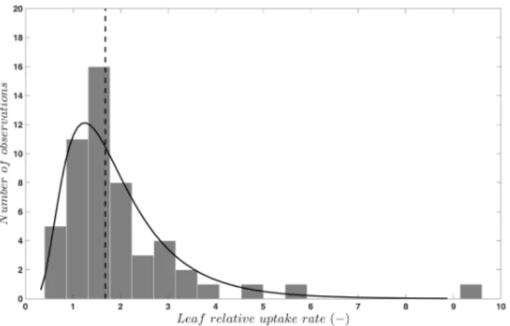
which cannot be observed directly. To keep the simplicity of the approach, especially when using OCS to evaluate models with many other built-in assumptions, the data-based LRU approximation is sufficient in many cases. We have compiled LRU data (n = 53) from an earlier review and merged them with more recent published studies (Berkelhammer et al., 2014; Stimler et al., 2010b, 2011, 2012). The LRUs com-piled in Sandoval-Soto et al. (2005) were partly re-calculated in Seibt et al. (2010) to account for the lower gas concen-trations in the sample cuvettes. For C3 plants, OCS uptake
behavior is attributed to CA activity (Yonemura et al., 2005). As shown in Fig. 2, LRU estimates for C3species under
well-illuminated conditions are positively skewed, with 95 % of the data between 0.7 to 6.2, which coincides with the theo-retically expected range of 0.6 to 4.3 (Wohlfahrt et al., 2012). The median, 1.68, is quite close to values reported and used in earlier studies and provides a solid “anchor ratio” for link-ing C3 plant OCS uptake and photosynthesis in high light.
LRU data are fewer for C4 species (n = 4), converging to
a median of 1.21, reflecting more efficient CO2uptake rates
compared to C3species (Stimler et al., 2011).
LRU remains fairly constant with changes in boundary layer and stomatal conductance but is expected to deviate due to changes in internal OCS conductance and CA activity (Seibt et al., 2010; Wohlfahrt et al., 2012). The primary en-vironmental driver of LRU is light, and an increase in LRU with decreasing photosynthetically active radiation has been observed at both the leaf (Stimler et al., 2010b, 2011) and ecosystem scale (Maseyk et al., 2014; Commane et al., 2015; Wehr et al., 2017; Yang et al., 2018). This behavior arises because photosynthetic CO2assimilation is reduced in low
light, whereas OCS uptake continues since the reaction with CA is not light dependent (Stimler et al., 2011). Note that since low light reduces CO2uptake, the flux-weighted effect
of the variations in LRU on estimating FCO2 (or GPP) is also
Figure 2. Frequency distribution (bars) and a lognormal fit (solid line) to published values (n = 53) of the leaf relative uptake rate of C3 species. The vertical line indicates the median (1.68). Pub-lished data are from Berkelhammer et al. (2014), Sandoval-Soto et al. (2005), Seibt et al. (2010), and Stimler et al. (2010b, 2011, 2012).
An additional complication is introduced by soil and non-vascular plant processes that both emit and consume OCS, with a few studies reporting net OCS emission under cer-tain conditions comparable in magnitude to net uptake rates during peak growth. Generally, soil OCS fluxes are low com-pared to plant uptake with a few exceptions (Fig. 3). In non-vascular plants, OCS uptake continues in the dark even when photosynthesis ceases (Gries et al., 1994; Kuhn et al., 1999; Kuhn and Kesselmeier, 2000; Gimeno et al., 2017; Rastogi et al., 2018). Unlike other plants, bryophytes and lichens lack responsive stomata and protective cuticles to control water losses. OCS emissions from these organisms seem to be pri-marily driven by temperature (Gimeno et al., 2017).
The yearly average land OCS flux rate in recent model-ing studies of global budgets (i.e., plant and soil uptake mi-nus soil emissions) ranges from −2.5 to −12.9 pmol m−2s−1 (Fig. 3). The only study reporting year-round OCS flux mea-surements is from a mixed temperate forest, which was a sink for OCS with a net flux of −4.7 pmol m−2s−1during the ob-servation period (Commane et al., 2015). Daily average OCS fluxes during the peak growing season are available from a larger selection of studies and cover the range from −8 to −23 pmol m−2s−1, excluding that of Xu et al. (2002), which found a surprisingly high uptake (–97 ± 11.7 pmol m−2s−1) from the relaxed eddy accumulation method (Fig. 3). Despite the limited temporal and spatial coverage, these data suggest that some of the larger global land net sink estimates may be too high (Launois et al., 2015b).
The following subsections explore a few aspects of ecosys-tem OCS exchange in greater detail. Observations and con-clusions about forests, grasslands, wetlands, and freshwater ecosystems are explored. Then we examine OCS
interac-tions reported for components of ecosystems: soils, micro-bial communities, and abiotic hydrolysis and sorption.
Recommendations. Available observations are limited in time and do not cover tropical ecosystems, which contribute almost 60 % of global GPP (Beer et al., 2010). More year-round measurements from a larger number of biomes, in particular those presently underrepresented, are required to provide reliable bottom-up estimates of the total net land OCS flux. The causes for the observed variability in Fig. 2 require more investigation because they hamper the spec-ification of defensible plant-functional-type-specific LRUs (Sandoval-Soto et al., 2005) and the development of models with non-constant LRU (Wohlfahrt et al., 2012). Relatively little is known regarding using OCS to estimate CA activity (Wehr et al., 2017), which is a promising new avenue of OCS research. Within this context, plant physiological and enzy-matic adaptations to increasing CO2and their effects on the
exchange of OCS are of special interest.
2.2.1 Forests
OCS has the potential to overcome many difficulties in study-ing the carbon balance of forest ecosystems. To partition carbon fluxes, respiration is often quantified at night, when photosynthesis has ceased and turbulent airflow is reduced (Reichstein et al., 2005). This method has systematic uncer-tainties; e.g., less respiration happens during the day than at night (Wehr et al., 2016). Partitioning with OCS is based on daytime data and does not rely on modeling respiration with limited nighttime flux measurements.
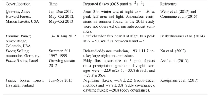
Forests are daytime net sinks for atmospheric OCS, when photosynthesis is occurring in the canopy (Table 1). While the relative uptake of OCS to CO2 by leaves appears
sta-ble in high-light conditions, the ratio changes in low light when the net CO2 uptake is reduced (Stimler et al., 2011;
Wehr et al., 2017; Rastogi et al., 2018). Forest soil interac-tion with OCS has been found to be small with respect to leaf uptake (Fig. 3) and straightforward to correct (Belviso et al., 2016; Wehr et al., 2017). Sun et al. (2016) noted that litter was the most important component of soil OCS fluxes in an oak woodland. Otherwise, forest ecosystem OCS up-take appears to be dominated by tree leaves, both during the day and at night (Kooijmans et al., 2017).
Recommendations. Tropical forest OCS fluxes would be informative for global OCS modeling efforts and are cur-rently absent from the literature. The OCS tracer approach is particularly useful in high-humidity or foggy environments like the tropics, where traditional estimates of carbon up-take variables via water vapor exchange are ineffective. Ad-ditionally, OCS observing towers upstream and downstream of large forested areas could resolve the synoptic-scale vari-ability in forest carbon uptake (Campbell et al., 2017b).
(a) (b) Global Forest Grassland Agriculture , June, Aug , July
Figure 3. Top panel: global average land OCS uptake from modeling studies. Bottom panel: reported averages and ranges of whole-ecosystem, site-level OCS observations. Points represent reported averages; error bars show the uncertainty around the average or the range of observed fluxes where no meaningful average was reported.
Table 1. In situ fluxes of forest ecosystems. Some of these data are plotted in Fig. 2.
Cover; location Time Reported fluxes (OCS pmol m−2s−1) Reference Quercus, Acer; Harvard Forest, Massachusetts, USA Jan–Dec 2011, May–Oct 2012, May–Oct 2013
Near 0 in winter and at night to ∼ −50 at peak leaf area and light. Anomalous emis-sions in summer found in the 2015 study were not observed during subsequent sum-mers.
Wehr et al. (2017) and Commane et al. (2015)
Populus, Pinus; Niwot Ridge, Colorado, USA
13–18 Aug 2012 Leaf chamber flux near 0 at night to a peak at ∼ −50; soil flux between 0 and −7.
Berkelhammer et al. (2014)
Picea; Solling mountains, Germany
Summer, fall 1997–1999
Relaxed eddy accumulation, −93 ± 11.7 up-take; large nighttime emissions.
Xu et al. (2002) Pinus; 3 sites, Israel Growing season
2012
Eddy flux covariance at 3 pine forests on a precipitation gradient; daylight aver-ages were −22.9 ± 23.5, −33.8 ± 33.1, and −27.8 ± 38.6.
Asaf et al. (2013)
Pinus; boreal forest, Hyytiälä, Finland
Jun–Nov 2015 Nighttime fluxes: −6.8 ± 2.2 (radon-tracer method) and −7.9 ± 3.8 (eddy covariance); daytime fluxes: −20.8 (eddy covariance).
2.2.2 Grasslands
OCS observations can address the need for additional stud-ies on primary productivity in grassland ecosystems. Grass-lands generally are considered to behave as carbon sinks or be carbon-neutral but appear highly sensitive to drought and heat waves and can rapidly shift from neutrality to a carbon source (Hoover and Rogers, 2016). Currently OCS grass-land studies are scarce (Fig. 3) but indicate a significant role for soils. Theoretical deposition velocities for grasses of 0.75 mm s−1 were reported by Kuhn et al. (1999), and LRU values of 2.0 were reported by Seibt et al. (2010). Whelan and Rhew (2016) made chamber-based estimates of ecosystem fluxes from a California grassland with a dis-tinct growing and non-growing season. Total ecosystem fluxes averaged −26 pmol m−2s−1 during the wet season and −6.1 pmol m−2s−1 during the dry season. During the wet season, simulated rainfall increased the sink strength. Light and dark flux estimates yielded similar sinks, sug-gesting either a large role for soils in the ecosystem flux or the presence of open stomata under dark conditions. Yi and Wang (2011) undertook chamber measurements over a grass lawn in subtropical China. Ecosystem fluxes of −19.2 pmol m−2s−1were observed. They noted average soil fluxes of −9.9 pmol m−2s−1 that were occasionally greater than 50 % of the total ecosystem flux. The large contribu-tion of soils to the grassland OCS flux was attributed to at-mospheric water stress on the plants that led to significant stomatal closure and reduced midday uptake by vegetation. More recently, Gerdel et al. (2017) reported daily average ecosystem-scale OCS fluxes of −28.7±9.9 pmol m−2s−1for a productive managed temperate grassland.
Solar radiation has been identified recently as a controlling factor of grassland soil OCS emissions. Kitz et al. (2017) highlighted that, in grasslands, primary production is de-voted to belowground biomass early in the growing season, leading to a situation where exposed soils may be emitting photo-produced OCS simultaneously with high GPP. If un-accounted for, this would lead to an underestimation of the plant component of the total ecosystem OCS flux (Kitz et al., 2017; Whelan and Rhew, 2016).
Recommendations. Grassland plants tend to include mix-tures of C3and C4species with a relative abundance and
im-portance to GPP evolving over the season. These different photosynthetic pathways are known to exhibit different LRU values. On the one hand, this poses a challenge to direct es-timations of GPP from OCS; on the other hand, observations may provide a unique opportunity to study C3 and C4
con-tributions to GPP. Another pressing research question is the effect of the changing leaf area index of grasses on radiation and related soil emissions.
2.2.3 Wetlands and peatlands
Much of the early work on OCS terrestrial–atmospheric fluxes was conducted in wetlands, perhaps because of the large emissions observed there. Unfortunately, many of these first surveys were conducted with sulfur-free sweep air, sig-nificantly biasing the observed net OCS flux compared with that under ambient conditions (Castro and Galloway, 1991).
OCS fluxes have been measured in a variety of wetland ecosystems, including peat bogs, coastal salt marshes, tidal flats, mangrove swamps, and freshwater marshes. Observed ecosystem emission rates vary by 2 orders of magnitude and generally increase with salinity (Fig. 4). OCS emissions in salt marshes usually range from 10 to 300 pmol m−2s−1 (Aneja et al., 1981; DeLaune et al., 2002; Li et al., 2016; Steudler and Peterson, 1984, 1985; Whelan et al., 2013), whereas freshwater marshes and bogs have mean emission rates below 10 pmol m−2s−1 (DeLaune et al., 2002; Fried et al., 1993) or act as net sinks due to plant uptake (Fried et al., 1993; Liu and Li, 2008; de Mello and Hines, 1994).
Although plants are generally OCS sinks, wetland plants may appear as OCS sources. Emergent stems can act as con-duits transmitting OCS produced in the soil to the atmo-sphere, or OCS may be a by-product of processes related to osmotic management by plants in saline environments. For example, in a Batis maritima coastal marsh, vegetated plots were found to have up to 4 times more OCS emission than soil-only plots (Whelan et al., 2013). Growing season OCS emissions may greatly exceed those in the non-growing sea-son (Li et al., 2016), but whether this is caused by environ-mental factors like temperature and soil saturation or by the developmental stage of plants is unclear.
Recommendations. Assessing the role of plants in the wet-land OCS budget would require careful investigation of OCS transport via plant stems and OCS producing capacity of aboveground plant materials and the rhizosphere. More work needs to be done on the evolution of OCS in soils with low redox potential. Additional experiments should aim to help scale up wetland OCS fluxes.
2.2.4 Lakes and rivers
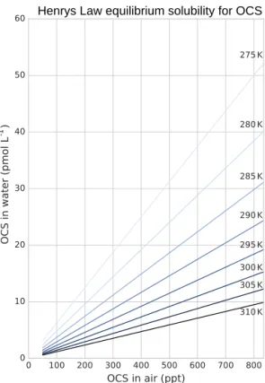
The role of lakes and rivers in the global OCS budget is not well known. OCS production and consumption have been studied in ocean waters, and these processes most likely oc-cur similarly in freshwater. In the ocean, OCS is produced photochemically from chromophoric dissolved organic mat-ter (CDOM) (Ferek and Andreae, 1984) and by a light-independent production that has been linked to sulfur radical formation (Flöck et al., 1997; Zhang et al., 1998). A mech-anism for OCS photoproduction was recently described for lake water (Du et al., 2017). Dissolved OCS (Fig. 5) is con-sumed by abiotic hydrolysis at a rate determined by pH, salinity, and temperature (Fig. 6; Elliott et al., 1989).
Fresh
Brakish
Saline
Figure 4. A summary figure for wetland OCS emissions. Lines indicate minimum to maximum ranges. Studies denoted “S” indicated a soil-only observation, and “S + V” denotes a soil and vegetation observation. Points show reported averages, and error bars show either reported uncertainty or the full range of observations. Note that some earlier observations using sulfur-free air as chamber sweep air have been excluded due to overestimation (Castro and Galloway, 1991).
Henrys Law equilibrium solubility for OCS
-1
Figure 5. Solubility of OCS in water dependent on ambient OCS concentration and temperature as calculated in Sun et al. (2015).
Temperature [°C] 0 5 10 15 20 25 30 Rate constant x10 -4 [s -1] 0 0.2 0.4 0.6 0.8 1 Elliott et al., 1989 Radford-Knoery et al., 1994 Kamyshny et al., 2003
Figure 6. Comparison of published hydrolysis rates for OCS based on laboratory experiments with artificial water (Elliott et al., 1989; Kamyshny et al., 2003), and under oceanographic conditions using filtered seawater (Radford-Kne¸ry et al., 1994). The graph is replot-ted using equations from original papers at a pH of 8.2.
OCS is present in freshwaters at much higher concentra-tions than those found in the ocean (Table 2). This might be due to more efficient mixing in the ocean surface waters com-pared to lakes. However, Richards et al. (1991) found that the concentration remained the same throughout the water column and observed a midsummer OCS concentration min-imum in 8 of the 11 studied lakes. This latter point was sur-prising because photochemical production should be high-est during the summer months. It has been demonstrated that ocean algae take up OCS, which might explain the low
con-centrations when light levels are high; however, Blezinger et al. (2000) concluded that the consumption term should be small compared to abiotic hydrolysis and photoproduction.
To our knowledge, there have not yet been any studies on OCS fluxes using direct flux measurement methods over freshwaters. Richards et al. (1991) calculated OCS fluxes from different lakes in Ontario, Canada, based on concen-tration measurements and wind-speed-dependent gas transfer coefficients, resulting in fluxes of 2–5 pmol OCS m−2s−1. In another study, Richards et al. (1994) found fluxes of 2– 34 pmol OCS m−2s−1 in salty lakes. These fluxes are 5 to 75 times higher than those measured in the oceans (Lennartz et al., 2017). There is also an indirect atmospheric OCS source from carbon disulfide (CS2) production (Richards
et al., 1991, 1994; Wang et al., 2001), for which little data exist.
Recommendations. Measurements in lakes are easier than in the open ocean while generating more information on the processes that may drive OCS production in both regions. Flux data by eddy covariance (EC) and floating chamber methods from lakes and rivers are suggested. Concurrent measurements should target understanding of the biotic and abiotic factors driving water–air exchange of OCS to provide the basis for upscaling aquatic OCS fluxes, including CS2
concentrations.
2.3 Other terrestrial OCS flux components
2.3.1 Soils
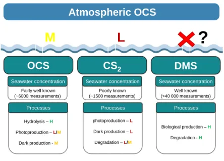
Measurements show that non-wetland soils are predomi-nantly a sink for OCS, and wetland (anoxic) soils are typ-ically a source of OCS. OCS production has also been ob-served in most non-desert oxic soils when dry, with particu-larly large emissions from agricultural soil (Fig. 7).
In the field, reported oxic soil OCS fluxes range from near zero up to −10 pmol m−2s−1, with average uptake rates typ-ically between 0 and −5 pmol m−2s−1. Higher uptake fluxes of −10 to −20 pmol m−2s−1have been observed in a grass-land soil (Whelan and Rhew, 2016), wheat field soils (Kanda et al., 1995; Maseyk et al., 2014), unplanted rice paddies (Yi et al., 2008), and bare lawn soil (Yi and Wang, 2011). How-ever, under warm and dry conditions, fluxes approached zero in grasslands (Berkelhammer et al., 2014; Whelan and Rhew, 2016) and an oak woodland (Sun et al., 2016). The highest re-ported uptake rates are nearly −40 pmol m−2s−1, following simulated rainfall in a grassland (Whelan and Rhew, 2016). Sun et al. (2016) also reported a rapid response to re-wetting following a rainstorm in a dry Mediterranean woodland.
Variations in soil OCS fluxes measured in the field have been linked to temperature, soil water content, nutrient sta-tus, and CO2fluxes. Uptake rates have been found to increase
with temperature (White et al., 2010; Yi et al., 2008) but also decrease with temperature such that OCS fluxes approached zero or shifted to emissions at temperatures around 15–20◦C
(Maseyk et al., 2014; Steinbacher et al., 2004; Whelan and Rhew, 2016; Yang et al., 2018). It can be difficult to separate the effects of temperature and soil water content in the field, and seasonal decreases in OCS fluxes may also be associated with lower soil water content (Steinbacher et al., 2004; Sun et al., 2016). Uptake rates have also been found to be stim-ulated by nutrient addition in the form of fertilizer or lime (Melillo and Steudler, 1989; Simmons, 1999).
Several field studies have found that OCS uptake is pos-itively correlated with rates of soil respiration, or CO2
pro-duction (Yi et al., 2007), but these relationships also vary with temperature (Sun et al., 2016, 2017), soil water content (Maseyk et al., 2014), or high-CO2conditions (Bunk et al.,
2017). The relationship with respiration is attributed to the role of microbial activity in OCS consumption, and simi-lar covariance has been seen between OCS and H2 uptake
(Belviso et al., 2013), a microbially driven process. Berkel-hammer et al. (2014) and Sun et al. (2017) have found that the OCS / CO2 flux ratio has a nonlinear relationship with
temperature, such that the ratio decreases (becomes more negative) at lower temperatures but is constant at higher temperatures. Kesselmeier and Hubert (2002) observed both OCS uptake and emission by beech leaf litter that was related to microbial respiration rates. Sun et al. (2016) determined that most of the soil OCS uptake in an oak woodland oc-curred in the litter layer, composing up to 90 % of the small surface sink.
Extensive laboratory studies demonstrate that OCS uptake is mainly governed by biological activity and physical con-straints. Kesselmeier et al. (1999), van Diest and Kesselmeier (2008), and Whelan et al. (2016) characterized the response of several controlling variables such as atmospheric OCS mixing ratios, temperature, and soil water content or water-filled pore space. Clear temperature and soil water content optima are observed for OCS consumption. These optima vary with soil type but indicate water limitation at low soil water content and diffusion resistance at high soil water con-tent. Additionally, other organism-mediated or abiotic pro-cesses in the soil, such as photo- or thermal degradation of soil organic matter (Whelan and Rhew, 2015), can play an important role.
The strong activity of sulfate reduction metabolism in anoxic environments is thought to drive OCS production in anoxic wetland soils (see Fig. 4) (Aneja et al., 1981; Kanda et al., 1992; Whelan et al., 2013; Yi et al., 2008). Tempera-ture probably drives the observed seasonal variation of OCS production, with higher fluxes in the summer than winter (Whelan et al., 2013). How much OCS escapes to the atmo-sphere depends on transport in the soil column. Tidal flood-ing may inhibit OCS emission from wetland soils due to de-creasing gas diffusivity with inde-creasing soil saturation rather than changes in OCS production rates (Whelan et al., 2013). With high light or temperatures, OCS production in oxic soils can exceed rates found in wetlands. Substantial OCS production has been observed in agricultural fields under
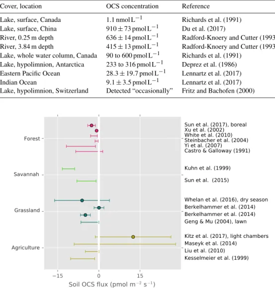
Table 2. OCS concentrations observed in rivers and lakes compared to ocean observations in Lennartz et al. (2017). Cover, location OCS concentration Reference
Lake, surface, Canada 1.1 nmol L−1 Richards et al. (1991) Lake, surface, China 910 ± 73 pmol L−1 Du et al. (2017)
River, 0.25 m depth 636 ± 14 pmol L−1 Radford-Knoery and Cutter (1993) River, 3.84 m depth 415 ± 13 pmol L−1 Radford-Knoery and Cutter (1993) Lake, whole water column, Canada 90 to 600 pmol L−1 Richards et al. (1991)
Lake, hypolimnion, Antarctica 233 to 316 pmol L−1 Deprez et al. (1986) Eastern Pacific Ocean 28.3 ± 19.7 pmol L−1 Lennartz et al. (2017) Indian Ocean 9.1 ± 3.5 pmol L−1 Lennartz et al. (2017) Lake, hypolimnion, Switzerland Detected “occasionally” Fritz and Bachofen (2000)
Forest
Savannah
Grassland
Agriculture
Figure 7. Field observations of soil OCS fluxes. Points are reported averages. Error bars are the reported range or the uncertainty of the average. Kuhn et al. (1999) represents an upper range due to under-pressurized soil chambers.
both wet and dry conditions (Kitz et al., 2017; Maseyk et al., 2014). OCS fluxes of up to +30 and +60 pmol m−2s−1 were related strongly to temperature (Maseyk et al., 2014) and radiation (Kitz et al., 2017), respectively. While most ecosystems do not experience these conditions, almost all soils produce OCS abiotically when air-dried and incubated in the laboratory (Whelan et al., 2016; Liu et al., 2010; Kaisermann et al., 2018; Meredith et al., 2018a). Whelan and Rhew (2015) compared sterilized and living soil sam-ples from the agricultural study site originally investigated in Maseyk et al. (2014), finding that all samples emitted consid-erable amounts of OCS under high ambient temperature and radiation, with even higher emissions after sterilization. Net OCS emissions can occur from agricultural soils at all water contents (Bunk et al., 2017) develop in summer (Yang et al., 2018), and OCS production rates do not differ significantly in moist and dry soils (Kaisermann et al., 2018). Meredith
et al. (2018a) found that OCS soil production rates are higher in low-pH, high-N soils that have relatively greater levels of microbial biosynthesis of S-containing amino acids and con-centrations of related S compounds.
Two mechanistic models for soil OCS exchange have been developed and can simulate observed features of soil OCS exchange, such as the responses of OCS uptake to soil water content, temperature, and the transition from OCS sink to source at high soil temperature (Ogée et al., 2016; Sun et al., 2015).
Both models resolve the vertical transport and the source and sink terms of OCS in soil layers. OCS uptake is repre-sented with the Michaelis–Menten enzyme kinetics, depen-dent on the OCS concentration in each soil layer, whereas OCS production is assumed to follow an exponential rela-tionship with soil temperature, consistent with field obser-vations (Maseyk et al., 2014). Although diffusion across soil
layers neither produces nor consumes OCS, altering the OCS concentration profile affects the concentration-dependent up-take of OCS.
Recommendations. Additional experiments are required to understand OCS production in oxic soils. The mechanism of soil production and why some soils are more prone to high production rates is unknown. In wetlands, the interaction between OCS production and transport processes remains poorly understood. If OCS produced by microbes accumu-lates in isolated soil pore spaces during inundation, subse-quent ventilation can lead to an abrupt release, which may appear as high variability in surface emissions. Field ex-periments using simple transport manipulation (e.g., straight tubes inserted into sediment) interpreted with soil modeling would clarify matters.
2.3.2 Microbial communities
The mechanism of OCS consumption in ecosystems is thought to be mediated by CA, a fairly ubiquitous en-zyme present within cyanobacteria, micro-algae, bacteria, and fungi. Purified from soil environments or from culture collections, bacteria and fungi show degradation of OCS at atmospheric concentrations. Mycobacterium spp. purified from soil and Dietzia maris NBRC15801T and Streptomyces ambofaciensNBRC12836T showed significant OCS degra-dation (Kato et al., 2008; Ogawa et al., 2016). Purified sapro-trophic fungi Fusarium solani and Trichoderma spp. were found to decrease atmospheric OCS (Li et al., 2010; Masaki et al., 2016). Some free-living saprophyte Sordariomycetes fungi and Actinomycetales bacteria, dominant in many soils, are also capable of degrading OCS (Harman et al., 2004; Nacke et al., 2011). Sterilized soil inoculated with Mycobac-teriumspp. showed the ability to take up OCS (Kato et al., 2008). In addition, cell-free extract of Acidianus spp. showed significant catalyzed destruction of OCS (Smeulders et al., 2011). During OCS degradation, soil bacteria introduce iso-topic fractionation (Kamezaki et al., 2016; Ogawa et al., 2017). Using different approaches, Bunk et al. (2017), Sauze et al. (2017), and Meredith et al. (2018b) showed that fungi might be the dominant player in soil OCS uptake.
In addition, there exist hyperdiverse microbial communi-ties that colonize the surface of plant leaves or the “phyl-losphere” (Vacher et al., 2016). The phyllosphere is an extremely large habitat (estimated in 1 billion km2) host-ing microbial population densities ranghost-ing from 105 to 107cells cm−2of leaf surface (Vorholt, 2012). With respect to OCS, it has already been shown that plant–fungal inter-actions can cause OCS emissions (Bloem et al., 2012). It is undetermined if these epiphytic microbes are capable of con-suming and emitting OCS.
Biotic OCS production is a possibility: in bacteria, novel enzymatic pathways have been described that degrade thio-cyanate and isothiothio-cyanate and render OCS as a byproduct (Bezsudnova et al., 2007; Hussain et al., 2013; Katayama
et al., 1992; Welte et al., 2016). Evidence for OCS emis-sions following SCN−degradation has been observed from
a range of environmental samples from aquatic and terres-trial origins, indicating a wide distribution of OCS-emitting microorganisms in nature (Yamasaki et al., 2002). Hydrol-ysis of isothiocyanate, another breakdown product of glu-cosinolates (Hanschen et al., 2014), by the SaxA protein also yields OCS, as shown in phytopathogenic Pectobacterium sp. (Welte et al., 2016). Some Actinomycetales bacteria and Mu-coromycotina fungi, both commonly found in soils, are also known to emit OCS, but the origin and pathway remains un-specified (Masaki et al., 2016; Ogawa et al., 2016).
Recommendations. Further studies should test the connec-tion between the microorganisms that degrade OCS and the candidate enzymes that we assume are performing the degra-dation. In addition, the magnitude of biotic OCS production in soils is unknown. While sterilized soils exhibit higher OCS production than live soils (Whelan and Rhew, 2015), we have not determined if biotic production is universally insignifi-cant in bulk soils.
2.3.3 Surface sorption and abiotic hydrolysis
Several abiotic processes can affect surface fluxes of OCS. OCS can be hydrolyzed in water and adsorb and desorb on solid surfaces. Abiotic hydrolysis of OCS in water oc-curs slowly relative to the timescales of typical flux ob-servations (Fig. 6). This is in contrast to the reaction in plant leaves, which is also technically a hydrolysis reac-tion but is catalyzed by CA. The temperature dependence of OCS solubility was modeled and described by Eq. (20) in Sun et al. (2015): for a OCS concentration in air of 500 ppt, in equilibrium at ambient temperatures, the OCS dissolved in water will be less than 0.5 pmol OCS / mol−1 H2O (Fig. 5). Some portion of the dissolved OCS is
de-stroyed by hydrolysis, following data generated by Elliott et al. (1989). For the rate-limiting step of hydrolysis in near-room-temperature water, the pseudo-first-order rate constant is around 2 × 10⁻⁵s−1. The hydrolysis of OCS gains signif-icance over hours, especially in ice cores (Aydin et al., 2014, 2016).
Under typical environmental conditions, OCS adsorp-tion and desorpadsorp-tion is near steady state. OCS adsorbs onto various mineral surfaces at ambient temperatures and can be desorbed at higher temperatures (Devai and DeLaune, 1997). In some ecosystems with large temperature swings, temperature-regulated sorption cannot be ruled out as play-ing a small role in the variability of observed fluxes.
Recommendations. Abiotic sorption has been overlooked in studies of OCS exchange. Observing fluxes while abruptly changing OCS concentrations over a sterile soil or litter sub-strate could reveal sorption’s role. This information could be used to inform our mechanistic soil models and explain some of the variability in OCS soil fluxes we see in the field.
Atmospheric OCS
DMS
?
Fairly well known (~6000 measurements) Seawater concentration Hydrolysis – H Photoproduction – L/M Dark production - M Processes Poorly known (~1500 measurements) Seawater concentration photoproduction – L Dark production – L Degradation – L/M Processes Well known (>40 000 measurements) Seawater concentration Biological production – H Degradation - H Processes
Level of understanding: H – high, M – medium, L - low
CS
2OCS
M
L
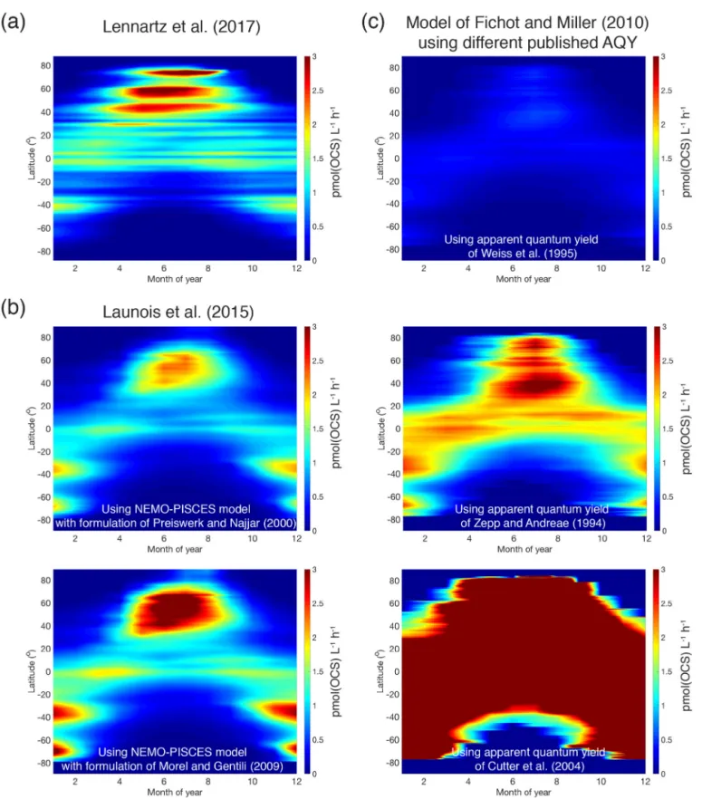
Figure 8. Marine contribution to the atmospheric OCS loading from direct and indirect (CS2) emissions. The sea surface concentration
deter-mines the magnitude of the oceanic emissions, and the uncertainty in global emissions decreases with increasing numbers of measurements. The understanding of processes is important to extrapolate from small-scale observations to a regional or global scale and varies between a low level of understanding for CS2(i.e., few process studies available) to a medium level of understanding for OCS (i.e., several process
studies available, but considerable spread in quantifications across different locations). We recommend reconsidering the contribution of oceanic DMS emissions.
2.4 Ocean
The oceans are known to contribute to the atmospheric bud-get of OCS directly via OCS and indirectly via CS2(Fig. 8)
(Chin and Davis, 1993; Watts, 2000; Kettle et al., 2002). Large uncertainties are still associated with current estimates of marine fluxes (Launois et al., 2015a; Lennartz et al., 2017, and references therein) and have led to diverging conclusions regarding the magnitude of their global role.
The range of observed OCS concentrations in surface wa-ters informs how the magnitude of direct oceanic emissions is calculated. Observations of OCS in the surface water of the Atlantic, Pacific, Indian, and Southern oceans revealed a consistent daily concentration range of ∼ 10–100 pmol L−1 in the surface mixed layer on average, across different meth-ods. Largest differences are found between coastal and es-tuaries (range: nanomoles per liter) and open oceans (range: picomoles per liter) (Table 3).
2.4.1 Marine production and removal processes
The primary sources of OCS in the ocean are divided into photochemical and light-independent (dark) processes (Von Hobe et al., 2001; Uher and Andreae, 1997). The primary sink is uncatalyzed hydrolysis (Fig. 6; Elliott et al., 1989). Evidence indicates that these processes can regulate OCS concentrations in the ocean surface mixed layer, with diverg-ing conclusions on the magnitude and global significance of
marine OCS emissions (Launois et al., 2015a). We use the Lennartz et al. (2017) budget here because the emission esti-mate is based on a model consistent with the majority of sea surface concentration measurements.
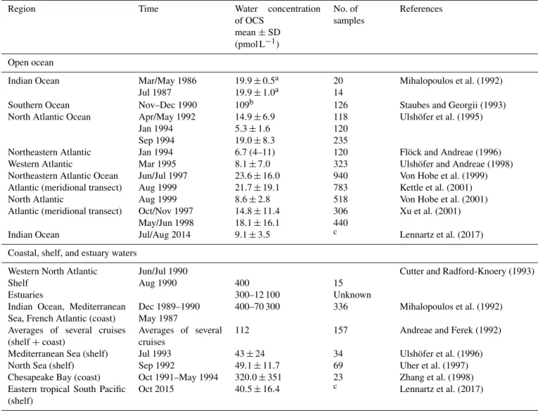
Global estimates of photoproduction for the surface mixed layer can range by up to a factor of 40 depending on the methodology used (Fig. 9). The heart of the problem is a lim-ited knowledge of the magnitude, spectral characteristics, and spatial and temporal variability of the apparent quantum yield (AQY).
There is evidence for the role of biological processes (Flöck and Andreae, 1996) and for the involvement of rad-icals (Pos et al., 1998) in OCS production. Independent of a mechanism, only one parameterization for dark production is currently used in models (Von Hobe et al., 2001). Neither the direct precursor nor the global applicability of this pa-rameterization is known. Despite these unknowns, the cur-rent gap in the top-down OCS budget (Sect. 3.1) is larger than the estimated ocean emissions, including uncertainties from process parameterization and in situ observations. This suggests that our estimates of OCS production in oceans will not close the gap in top-down OCS budgets.
Recommendations. Further studies should focus on gen-erating a biochemical model for estimating oceanic OCS fluxes. Refining uncertainty bounds for OCS photoproduc-tion could be facilitated by a comprehensive study of the vari-ability of AQYs across contrasting marine environments, the use of a photochemical model that utilizes AQYs and
facili-Figure 9. Comparison of OCS photoproduction rates (averages for surface mixed layer, pmol(OCS) L−1h−1) modeled using different approaches and demonstrating discrepancies between methods: (a) Hovmöller (latitude–time) plot of rates calculated using the approach described in Lennartz et al. (2017); (b) the same Hovmöller plot generated with the approach described in Launois et al. (2015a) and two different formulations for CDOM absorption coefficients from Preiswerk and Najjar (2000) and Morel and Gentili (2004); and (c) the same Hovmöller plots generated with the photochemical model of Fichot and Miller (2010) and the published spectral apparent quantum yields of Weiss et al. (1995), Zepp and Andreae (1994), and Cutter et al. (2004).
Table 3. Measurements of OCS water concentration at the ocean surface (0–5 m) in the open ocean as well as coastal, shelf, and estuary waters.
Region Time Water concentration of OCS mean ± SD (pmol L−1) No. of samples References Open ocean
Indian Ocean Mar/May 1986 Jul 1987 19.9 ± 0.5a 19.9 ± 1.0a 20 14 Mihalopoulos et al. (1992) Southern Ocean Nov–Dec 1990 109b 126 Staubes and Georgii (1993) North Atlantic Ocean Apr/May 1992
Jan 1994 Sep 1994 14.9 ± 6.9 5.3 ± 1.6 19.0 ± 8.3 118 120 235 Ulshöfer et al. (1995)
Northeastern Atlantic Jan 1994 6.7 (4–11) 120 Flöck and Andreae (1996) Western Atlantic Mar 1995 8.1 ± 7.0 323 Ulshöfer and Andreae (1998) Northeastern Atlantic Ocean Jun/Jul 1997 23.6 ± 16.0 940 Von Hobe et al. (1999) Atlantic (meridional transect) Aug 1999 21.7 ± 19.1 783 Kettle et al. (2001) North Atlantic Aug 1999 8.6 ± 2.8 518 Von Hobe et al. (2001) Atlantic (meridional transect) Oct/Nov 1997
May/Jun 1998 14.8 ± 11.4 18.1 ± 16.1 306 440 Xu et al. (2001) Indian Ocean Jul/Aug 2014 9.1 ± 3.5 c Lennartz et al. (2017) Coastal, shelf, and estuary waters
Western North Atlantic Shelf Estuaries Jun/Jul 1990 Aug 1990 400 300–12 100 15 Unknown
Cutter and Radford-Knoery (1993)
Indian Ocean, Mediterranean Sea, French Atlantic (coast)
Dec 1989–1990 May 1987
400–70 300 336 Mihalopoulos et al. (1992) Averages of several cruises
(shelf + coast)
Averages of several cruises
112 157 Andreae and Ferek (1992) Mediterranean Sea (shelf) Jul 1993 43 ± 24 34 Ulshöfer et al. (1996) North Sea (shelf) Sep 1992 49.1 ± 11.7 69 Uher et al. (1997) Chesapeake Bay (coast) Oct 1991–May 1994 320.0 ± 351 23 Zhang et al. (1998) Eastern tropical South Pacific
(shelf)
Oct 2015 40.5 ± 16.4 c Lennartz et al. (2017)
aConverted from ng L−1with a molar mass of OCS of 60.07 g. bConverted from ng S L−1with a molar mass of S of 32.1 g. cContinuous measurements.
tates calculations on a global scale, and the cross-validation of the depth-resolved modeled rates with direct in situ surements. During nighttime, continuous concentration mea-surements from research vessels can be used to calculate dark production rates assuming an equilibrium between hydroly-sis and dark production.
2.4.2 Indirect marine emissions
Indirect marine emissions from oxidation of the precursor gases CS2 and possibly dimethyl sulfide (DMS) were
hy-pothesized to be on the same order of magnitude as or larger than direct ocean emissions of OCS (Chin and Davis, 1993; Watts, 2000; Kettle et al., 2002). Production and loss pro-cesses of CS2in seawater are less well constrained than OCS
production, and they include photoproduction, evidence for
biological production (Xie et al., 1998, 1999), and a slow chemical sink (Elliott, 1990).
Measurements of CS2in the surface ocean comprise
sev-eral transects in the Atlantic and Pacific oceans with con-centrations in the lower picomoles-per-liter range. Signifi-cantly larger concentrations have been found in coastal wa-ters (Uher, 2006, and references therein). In laboratory ex-periments, Hynes et al. (1988) found that the OCS yield from CS2 increases with decreasing temperatures,
suggest-ing larger OCS production from CS2at high latitudes.
It is unclear if the ambient yield of OCS from DMS ox-idation is globally important. The production of OCS from the oxidation of DMS by OH has been observed in several chamber experiments, all of which used the same technique and experimental chamber (Barnes et al., 1994, 1996; Pa-troescu et al., 1998; Arsene et al., 1999, 2001) with a molar
yield of 0.7 ± 0.2 %. These studies were carried out at pre-cursor levels far exceeding those in the atmosphere (ppm), so the potential exists for radical–radical reactions that do not occur in nature. In addition, experiments took place in a quartz chamber on timescales that have potential for wall-mediated surface or heterogeneous reactions and using only a single total pressure and temperature (1000 mbar, 298 K). The mechanism and atmospheric relevance of OCS produc-tion from DMS remain highly uncertain.
Recommendations:To better constrain oceanic CS2
emis-sions, we suggest expanding surface concentration obser-vations across various biogeochemical regimes and sea-sons. Using field observations, laboratory studies, and pro-cess models, we could characterize production propro-cesses and identify drivers and rates when calculating OCS emission estimates. Elucidating the production pathway and validat-ing the atmospheric applicability of the reported OCS yields from DMS would require experiments at lower concentra-tions in a system that eliminates (or permits quantification of) wall-induced reactions.
2.5 Anthropogenic sources
Anthropogenic OCS sources include direct emissions of OCS and indirect sources from emissions of CS2. The
domi-nant source is from rayon production (Campbell et al., 2015), while other large sources include coal combustion, aluminum smelting, pigment production, shipping, tire wear, vehicle emissions, and coke production (Blake et al., 2008; Chin and Davis, 1993; Du et al., 2016; Lee and Brimblecombe, 2016; Watts, 2000; Zumkehr et al., 2017).
All recent global atmospheric modeling studies have used the low estimate of 180 Gg S yr−1from Kettle et al. (2002), which did not capture significant emissions from China. Updated globally gridded inventories are considerably higher: a bottom-up estimate of 223–586 Gg S yr−1for 2012 (Zumkehr et al., 2018) and a top-down assessment of 230 to 350 Gg S yr−1 for 2011 to 2013 (Campbell et al., 2015). One reason for the gap between the two recent inventories is that the top-down study used an optimization approach in which the result was limited to the a priori range, 150 to 364 Gg S yr−1. Both datasets indicate that most anthro-pogenic sources are in Asia.
Biomass burning is generally accounted for as a cate-gory separate from anthropogenic emissions. Several air-borne campaigns have observed increases in OCS concentra-tions in air masses from nearby burning events (Blake et al., 2008). The most recent estimate suggests that biofuels, open burning, and agriculture residue are 63, 26, and 11 % of the total OCS biomass burning emissions, respectively (Camp-bell et al., 2015).
Recommendations. Anthropogenic OCS emissions expe-rience large year-to-year variation (Campbell et al., 2017a). Ambient OCS monitoring and on-site industry observations in Asia could observe the anthropogenic contribution over
time. In particular, modern viscose-rayon factory emissions are necessary to capture the variability of emissions factors used to scale rayon production to OCS emissions using eco-nomic data.
2.6 Volcanic sources
OCS is emitted into the atmosphere by degassing magma, volcanic fumaroles, and geothermal fluids. OCS can be re-leased at room temperature by volcanic ash (Rasmussen et al., 1982) and has been observed to be conservative in the atmospheric plume emitted by the Mount Erebus volcano up to tens of kilometers downwind of the volcanic source (Op-penheimer et al., 2010).
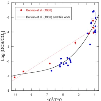
Using the linear relationship between the logarithm of the OCS / CO2ratio in volcanic gases and temperature, the
vol-canic OCS contribution was determined from estimated CO2
emissions (Belviso et al., 1986). Here we calculate a revised temperature dependence of log[OCS / CO2] with additional
data (Chiodini et al., 1991; Notsu and Toshiya, 2010; Sawyer et al., 2008; Symonds et al., 1992), as shown in Fig. 10. The compilation of measurements from 14 volcanoes shows that the former relationship from Belviso et al. (1986) overesti-mated the OCS / CO2ratio of volcanic gases with emission
temperatures from 110 to 400◦C, typical of extra-eruptive volcanoes. Even with this improved estimate, OCS emis-sions of extra-eruptive volcanoes are negligibly small and can definitely be discarded from the inventory of volcanic OCS emissions. Eruptive and post-eruptive volcanoes con-tribute almost all OCS emissions from volcanism.
Recommendations. An updated inventory of eruptive vol-canoes and a better assessment of their CO2emissions will
refine our understanding at a regional scale of the contribu-tion of OCS from volcanoes. Special attencontribu-tion should be paid to the Ring of Fire off the Asian continent where satellites have observed significant atmospheric OCS enhancements.
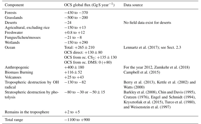
2.7 Bottom-up OCS budget
We calculate a “bottom-up” global balance of OCS with sev-eral approaches, as presented in Table 4. Within the atmo-sphere, the tropospheric sink owing to oxidation by OH is estimated to be in the range 82–130 Gg S yr−1(Berry et al., 2013; Kettle et al., 2002; Watts, 2000), and the stratospheric sink is in the range 30–80 Gg S yr−1, or 50 ± 15 Gg S yr−1 (Barkley et al., 2008; Chin and Davis, 1995; Crutzen, 1976; Engel and Schmidt, 1994; Krysztofiak et al., 2015; Turco et al., 1980; Weisenstein et al., 1997). OCS concentrations are increasing roughly 0.5–1 ppt year−1 averaged over the last 10 years (Campbell et al., 2017a), suggesting approxi-mately 2 to 5 Gg S yr−1remains in the troposphere.
We build a budget for terrestrial biomes that relies on ob-servations where available, and on estimates of carbon uptake where no data exists, as has been done previously (Camp-bell et al., 2008; Kettle et al., 2002; Suntharalingam et al.,
-8 -7 -6 -5 -4 -3 -2 1 3 5 7 9 11 Belviso et al. (1986)
Belviso et al. (1986) and this work
Lo g [O C S /C O ]2 103/T°C
Figure 10. Decimal logarithm of the OCS / CO2 ratios plotted
against the reciprocal of the emission temperature of the gases for volcanoes. The red dots refer to the analytical data published by Belviso et al. (1986) and the red line corresponds to the linear model used in that study to evaluate the volcanic contribution to the atmospheric OCS budget. The blue dots refer to measurements published by others since 1986 (Chiodini et al., 1991; Notsu and Toshiya, 2010; Sawyer et al., 2008; Symonds et al., 1992). The bet-ter fit through all measurements is obtained using a polynomial of the third order (R2=0.89, n = 31).
2008). In Table 5, the estimated OCS uptake is first calcu-lated from a GPP estimate and Eq. (1); then the net OCS flux is appraised by taking into account observed or esti-mated soil fluxes for each biome. The [CO2] and [OCS] are
assumed to be 400 ppm and 500 ppt, respectively, and LRU is 1.16±0.2 for C4plants (Stimler et al., 2010b) and 1.99±1.44
for C3plants (Fig. 2). We further assume a 150-day growing
season with 12 h of light per day for the purposes of con-verting between annual estimates of GPP and field measure-ments calculated in per-second units, though this obviously does not represent the diversity of biomes’ carbon assimila-tion patterns. Addiassimila-tionally, we assume that plants in desert biomes photosynthesize using the C4 pathway. Converting
annual estimated FCOS from an annual estimate to a
per-second estimate is sensitive to our growing season assump-tion. The lack of soil OCS flux time series datasets makes a more sophisticated upscaling approach ineffective. Antici-pated fluxes from soils and plants are therefore combined in this purposely simple method, scaled to the area of the biome extent, and presented in Table 4 as annual contributions to the atmospheric OCS budget.
We use a range of OCS flux observations in picomoles of OCS per square meter per second for fresh and saline wet-lands: −15 (de Mello and Hines, 1994) to +27 (Liu and Li, 2008) for freshwater wetlands and −9.5 (Li et al., 2016) to
+60 (Whelan et al., 2013) for saltwater wetlands (Fig. 4). Marine and inland wetlands cover 660 and 9200 × 103km2, respectively (Lehner and Döll, 2004). Performing a simple scaling exercise results in contributions of −140 to 250 and −6 to 40 Gg S yr−1for fresh and saltwater wetlands, respec-tively, yielding a total range of −150 to 290 Gg S yr−1 (Ta-ble 4).
To determine the role of non-vascular plant communities to the atmospheric OCS loading, we leverage Eq. (1) and work that has already been done on their carbon balance. According to Elbert et al. (2012), the annual contribution is 3.9 Pg C yr−1. A [OCS] of 500 ppt, a [CO2] of 400 ppm,
and a LRU of 1.1 ± 0.5 (Gimeno et al., 2017) yield −8 to −21 Gg S yr−1.
To estimate the maximum possible source of lakes to the atmospheric OCS burden, we perform a simple estimation of the global OCS flux following the approach in MacIntyre et al. (1995) as
FOCS=k(caq−ceq), (2)
where gas transfer coefficient, k, is assumed to be constant at 0.54 m d−1(Read et al., 2012); OCS concentration in the water, caq, is 90 pmol L−1 to 1.1 nmol L−1(Richards et al.,
1991); and OCS concentration in the surface water if it was in equilibrium with the above air, ceq, is calculated
us-ing Henry’s law at global average temperature of 15◦C and global atmospheric OCS mixing ratio of 500 ppt. Accounting for the number of ice-free days in a year and total lake surface area per latitude (Downing et al., 2006), the range of possible COS burden from lakes to the atmosphere is reported here as 0.8 to 12 Gg S yr−1.
Lennartz et al. (2017) generated a direct estimate of direct OCS emissions from oceans as 130 ± 80 Gg S yr−1. A mo-lar yield of CS2 to OCS of 0.81–0.93 was established by
Stickel et al. (1993) and Chin and Davis (1993), resulting in ocean OCS emissions from CS2 with an uncertainty of
20–80 Gg S yr−1. This uncertainty is from the emissions of CS2, not the molar yield, for which a globally constant factor
is used. The global DMS oxidation source of OCS was esti-mated by Barnes et al. (1994) as 50.1–140.3 Gg S yr−1, and subsequent budgets contain only revisions according to up-dated DMS emissions (Kettle et al., 2002; Watts, 2000). We suggest that the uncertainty in the production of OCS from DMS is underestimated. Until these issues are resolved, we recommend that this term be removed as a source from future budgets, but retained as an uncertainty.
Bottom-up analysis of the global anthropogenic inventory indicates a source of 500 ± 220 Gg S yr−1for the year 2012 (Zumkehr et al., 2018). The large uncertainty is primarily due to limited observations of emission factors, particularly for the rayon, pulp, and paper industries. The most recent esti-mate of the biomass burning sources is 116 ± 52 Gg S yr−1 (Campbell et al., 2015).
To calculate global volcanic OCS emissions, we first con-sider the range of global volcanic CO2 emission estimates
Table 4. Total bottom-up atmospheric OCS budget.
Component OCS global flux (Gg S year−1) Data source Forests −430 to −370
Grasslands −500 to −200
Deserts −24 No field data exist for deserts Agricultural, excluding rice −150 to +13
Freshwater +0.8 to +12 Fungus/lichen/mosses −21 to −8 Wetlands −150 to +290 Ocean Total: +265 ± 210
OCS direct: +130 ± 80 OCS from oc. CS2: +135 ± 130
OCS from oc. DMS: 0 (+80)
Lennartz et al. (2017); see Sect. 2.3
Anthropogenic +400 ± 180 For the year 2012, Zumkehr et al. (2018) Biomass Burning +116 ± 52 Campbell et al. (2015)
Volcanoes +25 to +43 Tropospheric destruction by OH
radical
−130 to −82 Berry et al. (2013), Kettle et al. (2002) and Watts (2000)
Stratospheric destruction by pho-tolysis
−80 to −30 or −50 ± 15 Barkley et al. (2008), Chin and Davis (1995), Crutzen (1976), Engel and Schmidt (1994), Krysztofiak et al. (2015), Turco et al. (1980), and Weisenstein et al. (1997)
Remains in the troposphere +2 to +5 Total range −1100 to +900
Table 5. GPP and OCS exchange estimates by biome. Biome GPP estimated by Beer et al. (2010) in Pg C yr−1 Biome area (109ha) Anticipated FOCS,
plants from GPP esti-mate (pmol m−2s−1) FOCS, soil (pmol m−2s−1) FOCS, ecosystem by GPP method (pmol m−2s−1) FOCS, ecosystem field observations (pmol m−2s−1) Tropical forests 40.8 1.75 −75 No dataa −83 to −73 No data Temperate forests 9.9 1.04 −30 −8 to 1.45b −38 to −29 ∼0 to 93h Boreal forests 8.3 1.37 −19 1.2 to 3.8c −18 to −16 0 to −22i Tropical savannas and
grasslands 31.3 2.76 −36 No data −61 to −29 No data Temperate grasslands and shrublands 8.5 1.78 −15 −25 to 7.3d −40 to −8 −26 growing season; +6.1 non-growing seasonj Deserts 6.4 2.77 −7 0 (?)e −7 (?) No data Tundra 1.6 0.56 −9 5.27 to 27.6f −4 to 18 −15 to −1k Croplands 14.8 1.35 −35 −18 to 40g −53 to 5 −22 to −16, +18 during non-growing seasonl Total 121.7 13.38
aFor the purpose of this estimate, we use the soil fluxes from temperate forests.
bRange of values from Castro and Galloway (1991), Steinbacher et al. (2004), White et al. (2010), and Yi et al. (2007).
cThe average reported here is the average and 1 SD from non-vegetated plots in a boreal forest, defined as plots having less than 10 % vegetation cover (Simmons, 1999).
dRange from Whelan and Rhew (2016). The error estimate here is different from the one reported because a different LRU was used. Kitz et al. (2017) found soil-only OCS production of
+60 pmol m−2s−1in an alpine grassland.
eIn a laboratory incubation study, Whelan et al. (2016) found that desert soils exhibit a very small uptake. No field measurements have been published to our knowledge. fThe smaller production is from de Mello and Hines (1994). The larger production is an average estimate from Fried et al. (1993).
gPost-harvest soil exchange estimate from the wheat field (Billesbach et al., 2014) investigated further in Whelan and Rhew (2015). hSee Table 1.
iFrom Simmons et al. (1999).
jRange from Whelan and Rhew (2016), encompassing observations of a grass field by Yi and Wang (2011).
kRange reported in de Mello and Hines (1994), encompassing values observed by a bog microcosm by Fried et al. (1993). No valid Arctic studies exist.
lHigh value for cotton, low value for wheat in Asaf et al. (2013). Daily fluxes for a wheat field investigated by Billesbach et al. (2014) were −21 during the growing season and +18 after harvest.