HAL Id: hal-01002603
https://hal-polytechnique.archives-ouvertes.fr/hal-01002603
Submitted on 7 Jul 2014
HAL is a multi-disciplinary open access
archive for the deposit and dissemination of
sci-entific research documents, whether they are
pub-lished or not. The documents may come from
teaching and research institutions in France or
abroad, or from public or private research centers.
L’archive ouverte pluridisciplinaire HAL, est
destinée au dépôt et à la diffusion de documents
scientifiques de niveau recherche, publiés ou non,
émanant des établissements d’enseignement et de
recherche français ou étrangers, des laboratoires
publics ou privés.
Time-resolved temperature rise in a thin liquid film due
to laser absorption
Maria Cordero, Emilie Verneuil, François Gallaire, Charles Baroud
To cite this version:
Maria Cordero, Emilie Verneuil, François Gallaire, Charles Baroud. Time-resolved temperature rise
in a thin liquid film due to laser absorption. Physical Review E : Statistical, Nonlinear, and Soft
Matter Physics, American Physical Society, 2009, 79 (1), pp.011201. �10.1103/physreve.79.011201�.
�hal-01002603�
Time-resolved temperature rise in a thin liquid film due to laser absorption
María Luisa Cordero,1Emilie Verneuil,1François Gallaire,2and Charles N. Baroud1,
*
1
LadHyX and Department of Mechanics, Ecole Polytechnique, 91128 Palaiseau, France 2
Laboratoire J. A. Dieudonné, Université de Nice Sophia-Antipolis, 06108 Nice, France
共Received 19 August 2008; published 7 January 2009兲
The temperature increase of a thin water layer is investigated, both experimentally and numerically, when the layer is heated by an infrared laser. The laser is focused to a waist of 5.3m inside a 28 m gap that contains fluorescent aqueous solutions between two glass slides. Temperature fields are measured using the temperature sensitivity of rhodamine-B, while correcting for thermal diffusion using rhodamine-101, which is insensitive to temperature. In the steady state, the shape of the hot region is well fitted with a Lorentzian function whose width ranges between 15 and 30m, increasing with laser power. At the same time, the maximum temperature rise ranges between 10 and 55 ° C and can display a decrease at high laser powers. The total energy stored in the sample increases linearly with the laser power. The dynamics of the heating occurs with two distinct time scales:共i兲 a fast time 共⌰= 4.2 ms in our case兲 which is the time taken to reach the maximum temperature at the laser position and the maximum temperature gradient, and共ii兲 a slow time scale for the spatial profile to reach its final width. The temperature field obtained numerically agrees quantitatively with the experiments for low laser powers but overpredicts the temperature rise while underpredicting the profile width for high powers. The total energy shows good agreement between experiments and simulations for all laser powers, suggesting that the discrepancies are due to a broadening of the laser, possibly due to a thermal lensing effect.
DOI:10.1103/PhysRevE.79.011201 PACS number共s兲: 44.10.⫹i, 66.25.⫹g
I. INTRODUCTION
Laser radiation offers a useful technique to heat an ab-sorbing sample in a localized way. Indeed, since a laser beam can be be focused to its diffraction limit, it can be used to inject energy at scales that are difficult to reach with other techniques, without requiring any specific microfabrication such as electrode deposition. Examples of applications where such heating has been applied include the evaporation of contaminants关1兴, the study of Marangoni flows 关2兴, the
mea-surement of media properties such as small absorbancies关3兴
and Soret coefficients关4兴, and the study of cell processes 关5兴
and of material properties under high pressure and tempera-ture conditions in diamond anvil cells关6兴. However, heating
can also appear as an undesirable side effect in optical ma-nipulation studies关7,8兴.
Recently, laser-induced heating was used to provide ac-tive control over droplet evolution in microfluidic channels, through the local manipulation of surface tension between water and oil 关9兴. In these studies, a laser was focused
through a microscope objective onto the surface of a water drop in order to locally vary the interfacial tension and thus create a Marangoni flow. The net force due to this flow pro-vides a way to control drop formation, routing, fusion, and division关10兴.
The potential usefulness of the laser heating is limited in two ways. First, it is important to quantify the dynamics of the temperature increase; even though miniaturization leads to a reduction of the thermal inertia and a shortening of the characteristic heating time, this time often needs to be com-pared with other short times, such as the time for the drop
interface to pass the laser position in the example of micro-fluidic drop control.
Second, many applications, such as thermophoresis or thermocapillarity, depend on the temperature gradient rather than the temperature itself, making it important to know the size of the region that is heated by the laser. Indeed, although the heating is localized, the width of the hot region is ex-pected to be larger than the size of the laser waist. Moreover, in practical applications of microfluidics or optical traps the temperature rise in the liquid can damage some biological samples or skew chemical measurements inside the micro-fluidic droplet.
In what follows, we concentrate on the heating of a thin liquid layer by a continuous wave laser that is focused to a small spot inside the sample. The presence of the top and bottom solid boundaries plays a fundamental role in the heat flux in our geometry, contrary to the assumptions in the ex-isting work on the subject which addresses a localized heat-ing in an infinite medium 关3,7,11–13兴. Fluorescence
mea-surements of temperature provide spatially and temporally resolved temperature fields 关14–16兴 and we correct for
ther-mally induced migration by developing a method based on two different fluorophores. This allows us to explore higher temperature ranges than in previous work 关17兴. Finally, the
experimental results are augmented by numerical solutions of the heat equation, which provide a way to explore differ-ent wall materials and layer thicknesses.
Below, we begin with a description of the experimental setup and method, followed by a theoretical treatment of the problem in Sec. III. The results of Sec.IVare divided into three parts, first describing the dynamics of the temperature rise in the transient regime, followed by the steady state spa-tial distribution, and finally by the results of the numerical simulation. The discussion summarizes the results and com-*charles.baroud@ladhyx.polytechnique.fr
ments on their utility for predicting the temperature field in specific cases.
II. EXPERIMENTAL SETUP
The experimental setup consists of an inverted micro-scope共Nikon ECLIPSE TE2000-U兲 with epifluorescent illu-mination from a metal halide lamp 共Exfo X-Cite 120兲, as shown in Fig. 1共a兲. An infrared laser beam of wavelength =1480 nm is collimated to a parallel Gaussian beam whose radius is measured at 1= 2.2 mm. The laser is focused in-side the sample through the microscope objective 共Nikon, Plan Fluor 10⫻ /0.3兲 of focal length f =20 mm to a Gaussian spot whose waist can be calculated, using Gaussian optics, to be 0=
冑
n12/关1+共Z1/ f兲2兴. Here, n=1.5 is the refractive in-dex of glass and Z1=12/, which yield
0= 5.3m. The laser power P0is measured at the sample position through a single glass slide and spans the range 10.5 to 132.8 mW.
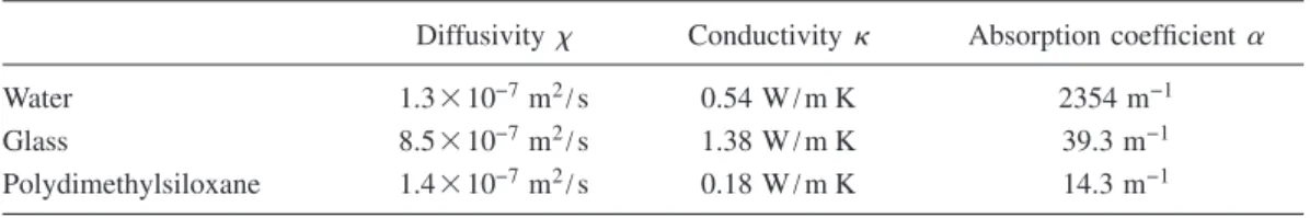
At this wavelength, part of the optical power is absorbed by the water, while the solid walls absorb almost none, as shown by the absorption coefficient␣ of TableI. This table also lists the thermal diffusivityand thermal conductivity for the three materials that will be discussed below.
Fluorescence images are recorded using a fast camera 共Photron Fastcam 1024 PCI兲, triggered by the same external signal as the laser, taking images at 500 frames per second. For each measurement, 50 images are recorded before the laser is switched on and averaged to be used as a room-temperature background. The fluorescence of the heated sample is then followed by recording 500 images after the trigger signal. The imaged region is a 1.74⫻1.74 mm
square. The spatial resolution of our measurements 共1.7m/pixel兲 is given by the microscope objective and the number of pixels on the camera sensor. The temporal reso-lution, on the other hand, is limited by the camera sensor’s sensitivity, which dictates the maximum frame rate that can still yield sufficient contrast between the hot and cold re-gions. For our conditions, this time is 2 ms.
The sample, sketched in Fig.1共b兲, consists of 200l of a fluorescent aqueous solution confined between two glass slides of diameter 76.2 cm and thickness H = 1 mm. A ring of a photoresist 共SU-8 2035, Microchem兲 of inner diameter 13 mm共not shown兲 is patterned on one of the glass slides by lithography and forms the chamber which contains the solu-tion and prevents its evaporasolu-tion. The height of the ring, 2h = 28m, was measured using a contact profilometer. Fi-nally, a 150 g weight is set on the upper glass slide to squeeze out the excess solution and seal the chamber. The resulting thickness of the liquid is small compared to the absorption length of the water 共400m兲, so that the Beer-Lambert law for laser absorption can be approximated by its linearization. The thickness is also small compared to the Rayleigh zone, LR=0
2/⬇130m, which defines the dis-tance over which the beam can be considered focused. The laser can therefore be considered divergence-free over this length.
A. Fluorophore solutions
Two different solutions are used in this study: the first is a rhodamine-B 共rho-B兲 aqueous solution 关Reactifs RAL, mo-lecular weight 共MW兲=479.02, 50 mg/l in 50M (4–共2–
FIG. 1. 共Color online兲 共a兲 Ex-perimental setup.共b兲 Lateral view of the sample共not to scale兲.
TABLE I. Thermal properties of the materials at room temperature. The material properties can vary with temperature.
Diffusivity Conductivity Absorption coefficient␣ Water 1.3⫻10−7m2/s 0.54 W/m K 2354 m−1
Glass 8.5⫻10−7m2/s 1.38 W/m K 39.3 m−1
Polydimethylsiloxane 1.4⫻10−7m2/s 0.18 W/m K 14.3 m−1
CORDERO et al. PHYSICAL REVIEW E 79, 011201共2009兲
hydroxyethyl兲-1–piperazineethanesulfonic acid) 共HEPES兲 buffer, pH = 7兴, whose fluorescence quantum yield 共emitted quanta per absorbed quanta兲 decreases with temperature 关18,19兴, and whose fluorescence variation can be calibrated
over a wide range of temperatures 关16兴. The second is an
aqueous solution of rhodamine-101 共rho-101兲 共Fluka, MW = 490.59, 30 mg/l in 50M HEPES buffer, pH = 7兲 whose fluorescence quantum yield is virtually independent of tem-perature关14,18,20兴. The two molecules are similar and have
a similar size, the main difference being the presence of di-ethylamino groups in the rho-B molecule, whose rotational freedom makes its quantum yield sensitive to temperature 关18兴.
The calibration of the fluorescence dependence of the rho-B solution on temperature is done, in the absence of the laser beam, by placing a 150 ml beaker of hot water on top of the glass slides. Thermal contact between the reservoir and the sample is provided by a layer of water, which allows us to consider that the sample temperature is the same as the beaker’s. The temperature of the water reservoir is monitored as it cools down from 80 ° C to room temperature. For every 1 ° C step, thirty images of the sample are taken at a frame rate of 500 frames/s and normalized by an image taken at room temperature, to correct for inhomogeneous illumina-tion. The fluorescence dependence on temperature is ob-tained as the spatial and temporal mean value over the 30 images, which is then fitted with a quadratic function, as shown in Fig.2. Note that the sample temperature is shifted to lower values with respect to the monitored temperature due to heat transfer into the surrounding air at room tempera-ture, the shift being higher at higher temperatures. This fact is estimated using a convection heat transfer model关21兴 due
to natural convection in the air and produces the error bars shown in Fig. 2.
B. Thermophoresis correction
When the laser is turned on, a decrease in fluorescence intensity around the laser focus is observed for both solu-tions. The details of the decrease, however, differ for the two dyes: In the case of rho-101, the dark central spot is sur-rounded by a bright ring at a radius r⬇50m, as shown in Fig.3共a兲. At later times, the dark spot continues to become
darker even after one second of heating关Fig.3共b兲兴. Simulta-neously, the ring expands and becomes less bright, in such a way that the total intensity, defined as the intensity integrated over the whole image, remains constant as a function of time 关Fig.3共c兲兴.
The azimuthal average of the rho-B solution, plotted in Fig.3共d兲, displays a stronger decrease than in the former case and no evidence of a bright ring is present. Furthermore, the fluorescence at the laser location initially decreases much faster, followed by a slower evolution关Fig.3共e兲兴. Finally, the total fluorescence intensity of rho-B is not conserved, as shown in Fig. 3共f兲, although the total fluorescence intensity returns to its initial value once the laser is switched off.
Since the rho-101 fluorescence quantum yield is not sen-sitive to temperature, the dark spot is solely due to a decrease in the concentration of dye molecules. This migration of molecules is due to their diffusion down the thermal gradi-ent, an effect known as thermophoresis, thermal diffusion or Soret effect关17,22兴. This is further confirmed by the
conser-vation of the total intensity, indicating that molecules have been redistributed through the sample, the bright ring corre-sponding to a radial accumulation of the molecules repelled from the high temperature region共“hot spot”兲. In the case of rho-B the fluorescence decrease is in part due to the tempera-ture dependence of its quantum yield, with thermophoresis responsible for an additional decrease in fluorescence at a slower time scale.
Since thermophoresis cannot be avoided in the presence of inhomogeneous thermal fields, the method we employ
0.5 0.6 0.7 0.8 0.9 1 20 30 40 50 60 70
fluorescence (arb. units)
temperature
(°
C)
measurements quadratic fit
FIG. 2. 共Color online兲 Temperature calibration of the rho-B so-lution fluorescence. 0 200 400 0.2 0.4 0.6 0.8 1 1.2 radius (µm) intensity (a) 0 0.5 1 0.2 0.4 0.6 0.8 1 time (s) intensity at r=0 (b) 0 0.5 1 0.96 0.98 1 1.02 1.04 time (s) tota li ntens ity (c) 0 200 400 0.2 0.4 0.6 0.8 1 1.2 radius (µm) intensity (d) 0 0.5 1 0.2 0.4 0.6 0.8 1 time (s) intensity at r=0 (e) 0 0.5 1 0.96 0.98 1 1.02 1.04 time (s) total intensity (f) Rhodamine 101 Rhodamine B
FIG. 3. 共Color online兲 共a兲, 共d兲 Radial fluorescence profiles after 1 s of laser heating with P0= 76.4 mW for the rho-101 and rho-B solutions, respectively. 共b兲, 共e兲 Fluorescence intensity at r=0 as a function of time for the rho-101 and rho-B solutions, respectively. 共c兲, 共f兲 Total fluorescence intensity as a function of time for the rho-101 and rho-B solutions respectively. Intensity scales are in arbitrary units.
takes advantage of the similarity in size between the two rhodamine molecules to correct the temperature and concen-tration dependence in the rho-B images by the strictly con-centration dependence for the rho-101. To that end, the same heating experiment is repeated using the two solutions and images are recorded with the same frame rate. The concen-tration variation is obtained from the rho-101 images, which is then used to normalize the rho-B image at each time step. In this way, temporally and spatially resolved temperature profiles are obtained.
III. THEORY
The theoretical description of the heating of a medium by absorption of a laser beam has been addressed by several authors in the past. The first analytical description was de-veloped by Carslaw and Jaeger in 1959关11兴, who solved the
heat equation for an infinitely extended opaque medium, heated by a Gaussian laser beam, using a Green’s function method. The result was later extended in 1965 by Gordon et al. 关3兴 for an infinitely long cylinder. However, neither
for-mulation takes into account the presence of top and bottom boundaries which play a major role in dissipating the heat. For this reason, the temperature increase predicted by both formulations highly exceeds our measurements.
More recent work describes the heating caused by the highly focused laser beams used in optical traps 关7,12,13兴.
Again, the effects of the boundaries are neglected, this time based on the fact that the laser absorption is produced in a spherical region of the size of the laser focus. For the high numerical aperture optics of optical traps, this is typically of the order of 1m, much smaller than the size of the cham-ber. In our system, however, the size of the heated volume is comparable to the chamber thickness and therefore a differ-ent model is necessary to describe the laser heating.
Consider a liquid layer, of thermal conductivity and thermal diffusivity , contained between two solid walls of thermal conductivitysand diffusivitys, as sketched in Fig.
1共b兲. The absorbing liquid is heated by a laser beam, focused at r = 0, of intensity I共r兲=2P0/0
2exp共−2r2/ 0
2兲. The total absorbed laser power is Pin= 2␣hP0, where ␣is the absorp-tion coefficient of the medium at the laser wavelength. The whole system is immersed in a thermal bath at room tem-perature. Since aⰇ0 and HⰇ2 h, the temperature rise is negligible at the lateral boundaries, r = a, and at the outer limits of the walls, z =⫾共H+h兲.
The elevation of temperature in the fluid, T, is described by the heat equation with a heat source term q˙ due to the laser absorption 关3,4,11兴: T t =ⵜ 2T + q˙, 共1兲 q˙⬇␣I共r兲, 共2兲 completed by the boundary conditions which account for the temperature and heat flux continuity at the fluid-solid bound-ary: T共r,z = ⫾ h,t兲 = Ts共r,z = ⫾ h,t兲, 共3兲
冉
T z冊
共r,z=⫾h,t兲=s冉
Ts z冊
共r,z=⫾h,t兲, 共4兲 where the subscript “s” indicates the values in the solid. The external temperature is assumed fixed. As Eqs. 共3兲 and 共4兲suggest, the temperature fields in the liquid and solid are coupled and one cannot be solved without the other. This system is easiest solved using numerical simulations, as done below in Sec.IV.
IV. RESULTS
A. Dynamics of the temperature increase
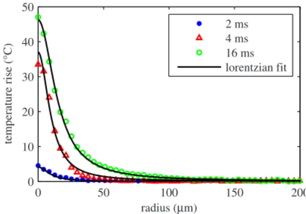
Three experimental depth-averaged temperature profiles are shown in Fig. 4 for an absorbed laser power Pin = 4.5 mW and times corresponding to 2, 4, and 16 ms after the laser is turned on. The temperature in the fluid rises nearly 50 ° C in a few milliseconds while the hot spot be-comes wider. However, the temperature increase remains less than 1.7 ° C at radii larger than 200m. The experimental data were accurately fitted by a Lorentzian curve:
T
¯ 共r,t兲 = ⌰共t兲
1 +关r/共t兲兴2, 共5兲 with two fitting parameters: ⌰共t兲, which corresponds to the temperature increase at the laser location, and共t兲, which is the half width at mid-height of the profile. This form of the temperature field agrees with those published by Duhr et al. 关23兴, although the laser powers are much larger here.
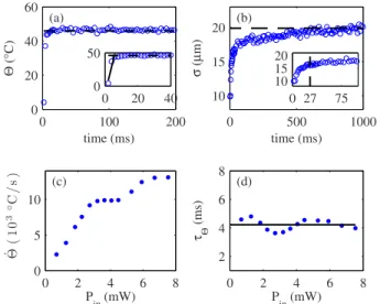
The evolution of⌰共t兲 and共t兲 is shown in Figs.5共a兲and
5共b兲, respectively. ⌰共t兲 increases rapidly, reaching its maxi-mum value⌰⬁within 10 ms. In contrast,共t兲 exhibits a fast increase at small times followed by a slower evolution, still slowly increasing after 1 s of laser heating. This increase is small, however, 共t兲 remaining around a value of 20m. For practical purposes, we will consider the steady state to be reached after 0.5 s of laser heating. It should be noted here that a slight difference between the thermophoretic behaviors of the two dyes may induce an error in the temperature field measurement that would be reflected in an unsteady value of 共t兲. 0 50 100 150 200 0 10 20 30 40 50 radius (µm) temperature rise (° C) 2 ms 4 ms 16 ms lorentzian fit
FIG. 4. 共Color online兲 Evolution of the radial temperature pro-file. The laser power is P0= 76.4 mW, which corresponds to an
absorbed power of Pin= 4.5 mW.
CORDERO et al. PHYSICAL REVIEW E 79, 011201共2009兲
The heating rate⌰˙ is arbitrarily defined as the slope of a linear fit of ⌰共t兲 for t艋6 ms 关see inset of Fig. 5共a兲兴. ⌰˙ increases with laser power, as seen in Fig.5共c兲, meaning that the rate of the temperature increase at the origin is larger for larger laser powers. Furthermore, a thermal time can be ex-tracted from this heating rate as⌰=⌰⬁/⌰˙. This time scale measures the time necessary to reach the maximum tempera-ture at the laser position. It is independent of the laser power, with a mean value具⌰典=4.2 ms, as shown in Fig.5共d兲.
Note that it is the gradient of temperature that determines thermocapillary effects. It is interesting therefore to measure the evolution of the gradient as a function of time. From the Lorentzian fit, the maximum thermal gradient occurs at a radius 共t兲/
冑
3 and its value −3冑
3⌰共t兲/8共t兲 is plotted in Fig.6. Indeed, the fast rise of the central temperature leads to a high value of the gradient at early times, which then as-ymptotes to its long term value as the hot spot spreads. The time to reach the maximum temperature gradient is well de-scribed by the time ⌰ for all laser powers. For Pin = 4.5 mW and t = 4 ms we find = 10m and ⌰=37 °C, yielding a thermal gradient of −2.4 ° C/m.B. Steady state
Next, we consider the depth-averaged temperature field at late times T¯⬁共r兲, which was computed by averaging the tem-perature distributions in the range 0.5⬍t⬍1 s. An example is shown in Fig. 7共a兲 for an absorbed laser power Pin = 4.5 mW. Again, the steady state radial profile is fitted by a Lorentzian curve that gives the temperature increase at the center⌰⬁and width ⬁of the hot spot as a function of Pin. Figure7共b兲shows that the amplitude⌰⬁ranges from 10 ° C for Pin= 0.68 mW to 55 ° C for Pin= 5.9 mW, before
decreas-ing again at higher laser powers. This nonlinear behavior is accompanied by a nonmonotonic increase of the steady state width of the hot spot⬁as a function of Pin, as shown in Fig.
7共c兲.
Note that the temperatures that are measured near the la-ser location for Pin⬎4 mW are outside the calibration range of Fig. 2. However, the values plotted in Fig. 7共b兲 are ob-tained from the fit over the whole temperature profile rather than actually observed at the spot center in the experiments. Since the profiles are well described by the Lorentzian curve, we assume that the values that are plotted correspond to the real physical temperatures.
Finally, the thermal energy⌬E stored by the sample, de-fined as ⌬E = 2h
冕
0 a T ¯ ⬁共r兲2r dr, 共6兲 was calculated by integrating the experimental temperature profiles.⌬E was found to increase linearly with the absorbed0 100 200 0 20 40 60 time (ms) Θ (° C) (a) 0 20 40 0 50 0 500 1000 10 15 20 time (ms) σ (µ m) (b) 0 27 75 10 15 20 0 2 4 6 8 0 5 10 Pin(mW) ˙ Θ( 10 3 ◦C/ s) (c) 0 2 4 6 8 2 4 6 8 Pin(mW) τ Θ (ms) (d)
FIG. 5. 共Color online兲 共a兲 ⌰共t兲 for Pin= 4.5 mW. The dashed
line indicates the maximum temperature increase⌰⬁. In the inset the first 40 ms are shown, and the solid line corresponds to a linear fit of the first points.共b兲 共t兲 for the same data. The dashed line indicates the value of⬁. The inset shows the first 100 ms.共c兲 ⌰˙ as a function of Pin.共d兲⌰as a function of Pin. The solid line indicates its mean value.
4 27 50 100 150 200 −2.5 −2 −1.5 −1 −0.5 0 time (ms) Thermal gradient (° C/ µ m)
FIG. 6. 共Color online兲 Evolution of the maximum thermal gra-dient after the laser is turned on, for an absorbed power Pin
= 4.5 mW. The gradient reaches its maximum absolute value at t = 4 ms. 0 100 200 0 20 40 radius (µm) temperature rise (° C ) (a) 0 2 4 6 8 0 20 40 60 Pin(mW) Θ ∞ (° C) (b) 0 2 4 6 8 10 20 30 P in(mW) σ ∞ (µ m ) (c) 0 2 4 6 8 0 0.1 0.2 P in(mW) ∆E (mJ) (d)
FIG. 7. 共Color online兲 共a兲 Dots: Radial temperature profile after 0.5 s of laser heating at Pin= 4.5 mW. Solid line: Lorentzian fit.共b兲 ⌰⬁ as a function of Pin.共c兲⬁ as a function of Pin.共d兲 ⌬E as a
function of Pin共dots兲 and linear fit 共solid line兲. For 共b兲–共d兲, the error bars here were calculated as the standard deviation of the data for all the time steps between 0.5⬍t⬍1 s.
laser power Pin关Fig.7共d兲兴, even in cases when the maximum temperature decreases. Indeed, the decrease in the value of the temperature near the laser focus is balanced by an in-crease in the size of the hot region in such a way that the total energy remains linear with the power. The slope of ⌬E共Pin兲 can be interpreted as a measure of the time required to reach a heat flux equilibrium between the injected energy and the heat dissipation into the solid walls, and therefore characterizes the time scale of establishment of the steady state. We measure this time as= 27 ms, in good agreement with the time taken for the temperature gradient to reach its steady value共Fig.6兲 and for the temperature profile to reach
its final width, as shown in the inset of Fig. 5共b兲 C. Numerical simulations
The system of Eqs.共1兲–共4兲 was solved numerically using
finite-element commercial software共COMSOL, Multiphysics兲 关24兴. The values extracted from the simulations were
com-pared with the experimental results, as shown in Fig. 8. Quantitative agreement is observed for low heating powers 共Pin⬍2 mW兲 for the maximum temperature increase 关Fig.
8共a兲兴, for the shape of the radial temperature profile 关Fig. 8共b兲兴, and for the evolution of the temperature increase at the
laser position⌰共t兲 关Fig. 8共c兲兴. This agreement breaks down at higher powers, with the simulations producing higher tem-peratures. Moreover, the width of the calculated temperature profiles remains almost constant at about 10m, therefore failing to account for the broadening of the profile that is observed in the experiments. However, the calculation of the total stored energy yields a good agreement between the ex-periments and simulations for all laser powers 关Fig.8共d兲兴.
The good agreement between the measurements and the numerical simulations at low laser powers suggests that the
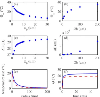
numerical calculations can be used to describe the heating for different values of the parameters. The values of⌰⬁and of ⌬E are shown as a function of the laser waist and the depth of the liquid film in Figs. 9共a兲–9共d兲. While the tem-perature increase is very sensitive to both 0 and h 关Figs.
9共a兲and9共b兲兴, the thermal energy depends only weakly on
0关Fig.9共c兲兴, but strongly on h 关Fig.9共d兲兴.
These results may explain the discrepancy between the measured and simulated temperature profiles, which disagree in the value of⌰⬁while the total energy shows good agree-ment. This is coherent with a widening of the laser spot in the experiments, which may be due to the creation of a di-verging thermal lens in the lower glass slide as its tempera-ture rises关3兴. Such a thermal lens would depend on
tempera-ture, which accounts for the increasing discrepancy at high laser powers. Evidence of the existence of this thermal lens can be seen when the sample is viewed with transmitted white light; the location of the laser appears darker than the rest, indicating that the material acts to diverge the light.
Finally, the numerical method is used to calculate the tem-perature increase in a layer of water enclosed between one glass slide and one polydimethylsiloxane共PDMS兲 wall, as in the case of a microfluidic device 关9,10兴. The value of the
thermal conductivity for PDMS is significantly lower than the value for glass 共see TableI兲, implying that heat will be
evacuated less efficiently in the PDMS wall. Consequently, the temperature increase is higher and more extended in this case, as shown in Fig.9共e兲. However, the time scale for the increase of ⌰共t兲, shown in Fig. 9共f兲, is not significantly modified by the different boundary conditions.
0 2 4 6 8 0 20 40 60 80 Pin(mW) Θ ∞ (° C) (a) 0 100 200 0 20 40 60 radius (µm) temperature rise (° C ) (b) 0 0.05 0.1 0 10 20 time (s) Θ (° C) (c) 0 2 4 6 8 0 0.1 0.2 Pin(mW) ∆E (mJ) (d)
FIG. 8. 共Color online兲 Comparison between the experimental and the numerical results. 共a兲 ⌰⬁ as a function of Pin. The dots correspond to the measurements and the triangles to the numerical simulations. 共b兲 Experimentally and numerically obtained radial temperature profiles T¯⬁共r兲 for Pin= 1.3 mW共circles and solid line兲
and Pin= 4.1 mW 共stars and dashed line兲. 共c兲 ⌰共t兲 for Pin = 1.3 mW. The dots correspond to the experiment and the solid line to the simulation.共d兲 ⌬E as a function of Pinobtained by the ex-periments共dots兲 and by the simulations 共triangles兲.
0 10 20 30 0 20 40 ω0(µm) Θ ∞ (° C) (a) 0 100 200 0 20 40 2h (µm) Θ ∞ (° C) (b) 0 10 20 30 27 28 29 30 ω0(µm) ∆E( µJ) (c) 0 100 200 0 1 2x 10 6 2h (µm) ∆E (mJ) (d) 0 100 200 0 10 20 radius (µm) temperature rise (° C) (e) 0 20 40 0 10 20 30 time (ms) Θ (° C) (f)
FIG. 9. 共Color online兲 Simulated variations of the main param-eters for a laser power P0= 20 mW.共a兲,共b兲 ⌰⬁as a function of0 and 2h, respectively.共c兲,共d兲 ⌬E as a function of0and 2h,
respec-tively. 共e兲,共f兲 Comparison between T¯⬁共r兲 and ⌰共t兲 for two glass walls共dashed lines兲 and a combination of one glass and one PDMS wall共solid lines兲, as in the case of a microchannel.
CORDERO et al. PHYSICAL REVIEW E 79, 011201共2009兲
V. DISCUSSION
The establishment of a temperature profile by laser heat-ing takes place over several time scales. The fastest one cor-responds to the central laser region reaching its final tem-perature, which also sets the time required to reach the maximum temperature gradient. This time scale is indepen-dent of the laser power and is measured at⌰= 4.2 ms in our experiments. Later, the establishment of the width of the Lorentzian profile occurs over a longer time which is asso-ciated with the diffusion of the heat into the solid walls; this time will vary with the material properties, although it is also independent of laser power. In our experiments, we measure = 27 ms.
The profile is well described by a Lorentzian curve and the experiments display a nontrivial balance between the width of the hot spot and the height of the temperature peak. These results are not recovered in the numerical simulations, suggesting that the transmission of the laser through the dif-ferent media is affected by the temperature variations.
Our measurements and simulations can be efficiently used to describe experiments involving laser heating by providing a useful basis for understanding its limitations. Indeed, the steady state profile measured here should still provide a good approximation of the profile expected in the presence of fluid
flows, as long as heat diffusion remains faster than advec-tion. This is quantified by the thermal Peclet number Pe = UL/, where U is a characteristic velocity and L a charac-teristic length scale which can be taken as L =⬁, the width of the hot spot. Therefore, by using the values for water and in the conditions discussed in this paper, we find that Pe ⬍1 for characteristic velocities U⬍1 cm/s, which is the case in the previous studies on laser-induced droplet manipu-lation by thermocapillarity关9,10,25兴.
Finally, note that our measurements do not take into ac-count the vertical variation of temperature. The numerical solutions show a strong thermal gradient in the z direction, which depends on the material properties of the walls, as was previously shown关17兴. These variations should be taken into
account if a more precise model of the effect of the ther-mocapillary flow is needed.
ACKNOWLEDGMENTS
The authors acknowledge Antigoni Alexandrou for help in the optical measurements. This work was partially funded by the convention X-DGA. M.L.C. was funded by the EADS Corporate Foundation and by MIDEPLAN. E.V. was funded by the CNRS.
关1兴 K. Fushinobu, L. M. Phinney, and N. C. Tien, Int. J. Heat Mass Transfer 39, 3181共1996兲.
关2兴 G. Da Costa, Appl. Opt. 32, 2143 共1993兲.
关3兴 J. P. Gordon, R. C. C. Leite, R. S. Moore, S. P. S. Porto, and J. R. Whinnery, J. Appl. Phys. 36, 3共1965兲.
关4兴 R. Rusconi, L. Isa, and R. Piazza, J. Opt. Soc. Am. B 21, 605 共2004兲.
关5兴 H. Reinhardt, P. S. Dittrich, A. Manz, and J. Franzke, Lab Chip 7, 1509共2007兲.
关6兴 L.-C. Ming and W. A. Bassett, Rev. Sci. Instrum. 45, 1115 共1974兲.
关7兴 H. Mao, J. R. Arias-Gonzalez, S. B. Smith, I. J. Tinoco, and C. Bustamante, Biophys. J. 89, 1308共2005兲.
关8兴 S. Ebert, K. Travis, B. Lincoln, and J. Guck, Opt. Express 15, 15493共2007兲.
关9兴 C. N. Baroud, J.-P. Delville, F. Gallaire, and R. Wunenburger, Phys. Rev. E 75, 046302共2007兲.
关10兴 C. N. Baroud, M. R. de Saint Vincent, and J.-P. Delville, Lab Chip 7, 1029共2007兲.
关11兴 H. S. Carslaw and J. C. Jaeger, Conduction of Heat in Solids 共Clarendon Press, Oxford, 1959兲.
关12兴 Y. Liu, D. K. Cheng, G. J. Sonek, M. W. Berns, C. F. Chap-man, and B. J. Tromberg, Biophys. J. 68, 2137共1995兲.
关13兴 E. J. G. Peterman, F. Gittes, and C. F. Schmidt, Biophys. J. 84, 1308共2003兲.
关14兴 J. Sakakibara, K. Hishida, and M. Maeda, Int. J. Heat Mass Transfer 40, 3163共1997兲.
关15兴 R. Zondervan, F. Kulzer, H. van der Meer, J. A. J. M. Dissel-horst, and M. Orrit, Biophys. J. 90, 2958共2006兲.
关16兴 D. Ross, M. Gaitan, and L. Locascio, Anal. Chem. 73, 4117 共2001兲.
关17兴 S. Duhr and D. Braun, Eur. Phys. J. E 15, 277 共2004兲. 关18兴 T. Karstens and K. Kobs, J. Phys. Chem. 84, 1871 共1980兲. 关19兴 K. G. Casey and E. L. Quitevis, J. Phys. Chem. 92, 6590
共1988兲.
关20兴 A. Marcano and O. Urdaneta, Appl. Phys. B: Lasers Opt. 72, 207共2001兲.
关21兴 F. P. Incropera and D. P. De Witt, Fundamentals of Heat and
Mass Transfer, 2nd ed.共John Wiley & Sons, New York, 1985兲.
关22兴 S. Duhr and D. Braun, Phys. Rev. Lett. 96, 168301 共2006兲. 关23兴 S. Duhr and D. Braun, Phys. Rev. Lett. 97, 038103 共2006兲. 关24兴 See EPAPS Document No. E-PLEEE8-78-183812 for a
de-scription of the numerical simulation. For more information on EPAPS, see http://www.aip.org/pubservs/epaps.html.
关25兴 M. R. de Saint Vincent, R. Wunenburger, and J.-P. Delville, Appl. Phys. Lett. 92, 154105共2008兲.