Absolute sensitivity calibration of an extreme ultraviolet spectrometer for tokamak measurements

HAL Id: hal-01369758

https://hal.archives-ouvertes.fr/hal-01369758

HAL is a multi-disciplinary open access archive for the deposit and dissemination of sci-entific research documents, whether they are pub-lished or not. The documents may come from teaching and research institutions in France or abroad, or from public or private research centers.

L’archive ouverte pluridisciplinaire HAL, est destinée au dépôt et à la diffusion de documents scientifiques de niveau recherche, publiés ou non, émanant des établissements d’enseignement et de recherche français ou étrangers, des laboratoires publics ou privés.

Absolute sensitivity calibration of an extreme ultraviolet

spectrometer for tokamak measurements

R Guirlet, Jl Schwob, O Meyer, S Vartanian

To cite this version:

R Guirlet, Jl Schwob, O Meyer, S Vartanian. Absolute sensitivity calibration of an extreme ultraviolet spectrometer for tokamak measurements . 2016. �hal-01369758�

1

Absolute sensitivity calibration of an extreme ultraviolet spectrometer for tokamak 1

measurements 2

R. Guirleta,1, JL. Schwobb, O. Meyera, S. Vartaniana 3

a

CEA, IRFM, F-13108 St-Paul-lez-Durance, France 4

b

Racah Institute of Physics, Hebrew University of Jerusalem, Israel 5

6

Abstract 7

An extreme ultraviolet spectrometer installed on the Tore Supra tokamak has been 8

calibrated in absolute units of brightness in the range 10-340 Å. This has been performed by 9

means of a combination of techniques. The range 10-113 Å was absolutely calibrated by using 10

an ultrasoft-X ray source emitting six spectral lines in this range. The calibration transfer to 11

the range 113-182 Å was performed using the spectral line intensity branching ratio method. 12

The range 182-340 Å was calibrated thanks to radiative-collisional modelling of spectral line 13

intensity ratios. The maximum sensitivity of the spectrometer was found to lie around 100 Å. 14

Around this wavelength, the sensitivity is fairly flat in a 80 Å wide interval. The spatial 15

variations of sensitivity along the detector assembly were also measured. The observed trend 16

is related to the quantum efficiency decrease as the angle of the incoming photon trajectories 17

becomes more grazing. 18

19

Keywords: extreme ultraviolet; spectroscopy; tokamaks; absolute calibration 20

21

1. Introduction 22

23

Extreme ultraviolet (EUV) spectroscopy is used extensively in various plasma physics 24

research fields such as astrophysics and inertial and magnetic fusion. Its main interest resides 25

in the detailed information it provides on the various species present in a plasma. It thus helps 26

determine the qualitative composition of a plasma by the observation and identification of the 27

spectral lines emitted by the ion species of the plasma. The density of the various emitting 28

ions can also be deduced from spectroscopic measurements provided certain experimental 29

conditions are fulfilled. One of them is that the spectral line intensities must be measured in 30

absolute units. This necessitates that the spectroscopic instrument be calibrated in sensitivity. 31

1 _{Corresponding author. Tel.: +33-442-25-38-85.}

2

A commonly used method is the so-called line intensity branching ratio method [1, 2]. 32

It consists of selecting spectral line pairs emitted by the same ion from one given upper level 33

to two different lower levels and comparing their measured intensity ratio with the theoretical 34

one. For this purpose, usually the spectrometer to be calibrated includes a visible line of sight 35

as close as possible to the EUV line of sight and connected to a visible spectrometer (for 36

which an absolute calibration is relatively easy). One line of the pair is chosen in the visible 37

range, and thus the sensitivity of the EUV spectrometer at the second line wavelength can be 38

deduced. This method has been used already many years ago on the TA 2000 torus [3, 4] and 39

is still in use nowadays, for example at JET for the SPRED VUV spectrometer in the range 40

130-360 Å [5]. Another way of calibrating an EUV spectrometer in absolute intensity units is 41

to compare the spectrometer signals with those of an already absolutely calibrated instrument, 42

as was done in [6] in the soft-X ray range. 43

In the present work, the Tore Supra tokamak is equipped with a high resolution, duo-44

multichannel grazing incidence spectrometer [7] of the Schwob-Fraenkel type. Two 45

interferometrically aligned, ruled, concave gratings are mounted permanently on the 46

spectrometer. For most of the applications and in particular for the present measurements, a 47

600 g/mm grating blazed at 1.5° is used. It covers the 10-340 Å wavelength range. The 48

spectrometer is supported by a mobile structure which allows to spatially scan the lower half 49

of the plasma at a frequency 0.5 Hz. 50

Detection on this spectrometer is performed by means of two double microchannel 51

plate (MCP) detector assemblies in chevron configuration mounted on two carriages moved 52

independently along the materialised Rowland circle. The range of one detector is limited on 53

one end by the shortest wavelength mechanically accessible and on the other end by the 54

second detector assembly. It is thus called the 'short wavelength' (or SW) detector. 55

Conversely, the other assembly is limited by the SW detector and the longest wavelength 56

mechanically accessible, hence its name: 'long wavelenth' (or LW) detector. The electrons 57

produced in the microchannels by impact of the incident EUV photons are converted into 58

visible photons by phosphor screens behind the MCPs and recorded by PDA (photodiode 59

array) cameras (one for either MCP assembly). An example of a spectrum recorded on the 60

LW detector is shown in Fig. 1. 61

3 62

Figure 1: Spectrum recorded by the long wavelength detector with identification of the 63

most prominent lines.

64 65

This spectrometer is not built with a visible line of sight so we could not use the 66

branching ratio method exactly as presented in [1]. For the short wavelength part of the 67

accessible domain we have used a combination of methods which are reported in this article. 68

Section 2 describes the use of an ultrasoft-X ray source for absolute calibration in the 10-113 69

Å range. Section 3 describes the method used for calibration in the longer wavelength range, 70

which combines the branching ratio method with a comparison of line intensity ratio 71

measurements with collisional-radiative calculations, a method already used in [8]. Section 4 72

contains the results with a discussion on the uncertainties and a study of the spatial variation 73

of the detector sensitivity. Section 5 presents a summary and conclusions. 74

75

76

2. Sensitivity calibration in the short wavelength range 77

78

2.1 Experimental setup and method 79

80 81

4 82

Figure 2: Absolute calibration setup with the ultrasoft-X ray Manson source 83

84

Target element Wavelength (Å)

Mg 9.9 O 23.7 N 31.6 C 44.4 B 67.0 Be 113.0 85

Table 1: List of emitting elements in the various targets and wavelengths of the 86

corresponding spectral lines.

87 88

In the short wavelength range, an absolute calibration was performed in the 89

spectroscopy laboratory with the help of a Manson Model 5 multi-anode ultrasoft-X ray 90

source [9]. The set-up is sketched on Fig. 2. The source emits photons at a given wavelength 91

(the so-called Kα line) by electron beam impact on targets (playing the role of anodes for the 92

electrons) of various materials. A carousel of six targets allows to produce as many spectral 93

lines between 9.9 and 113 Å (see Table 1). 94

A gas flow proportional counter (GPC) is placed at 45° from the electron beam axis (a 95

setup very similar to the one used in [10]) to monitor the photon emission which can be as 96

high as 1012 photons/(s.sr). The GPC is set up so that it has a 100% efficiency. In order to 97

preserve its operating pressure, which is different from that in the source volume, a membrane 98 e- hν Gas flow proportional counter EUV spectrometer Target

Ultrasoft-X ray source hν

Vacuum pipes Membrane

5

is placed in front of the counter as a separation from the source volume. The membrane 99

transmission factor TGPC depends on the wavelength, as shown in Table 2.

100 101

Wavelength (Å) 9.9 23.7 31.6 44.4 67.0 113.0

TGPC (%) 55 42 32 19 50 37

102

Table 2: transmission factor of the membrane in front of the gas flow proportional counter 103

104

In addition, we have used a grid filter (transmission TF = 0.108) to attenuate the GPC

105

signal. The photon rate (in s-1) measured by the GPC is thus given by: 106 ) ( ) ( ) (λ GPC λ F GPCi λ m GPC T T N N = × × (1) 107 108

where NiGPC(

λ

λ

109

The spectrometer beam line is placed in a position symmetric to the GPC with respect 110

to the electron beam to take advantage of the photon emission symmetry around the electron 111

beam axis. The ratio of the photon rate incident on the spectrometer Nspi(λ) to the photon rate

112

NiGPC(

λ

113 detectors: 114 GPC sp i GPC i sp N N Ω Ω = ) ( ) (

λ

λ

Note here that Nspi(

λ

117

width excluding the background in the same spectral interval. 118

The spectrometer sensitivity at wavelength λ is defined as the ratio of the measured count rate 119

to the incident photon rate: 120 ) ( ) ( ) (

λ

λ

λ

η

where Nspm(

λ

122

(expressed in counts/s in our setup). Due to the 100% efficiency of the gas counter and using 123

Eqs. 1 and 2, one has: 124 F GPC m GPC GPC sp i GPC GPC sp i sp T T N N N ) ( ) ( ) ( ) (

λ

λ

λ

λ

6

(

)

The spectrometer sensitivity can thus be deduced from the geometric parameters of the setup, 129

which are known, and the measurements of the detectors. 130

131

The tokamak plasma observed with the spectrometer is an extended light source. The 132

measurement performed by the spectrometer is thus the radiance (also commonly called 133

brightness) defined as: 134

( )

∫

( )

where ε (in cm-3s-1), called emissivity, is the photon rate emitted by plasma unit volume in a 137

given spectral line and l is the abscissa along the line of sight. The integral is performed over

138

the whole line of sight path within the plasma. The quantity we aim at determining is the 139

brightness calibration coefficient K(

λ

140 141

( )

( )

( )

over the whole wavelength range of the spectrometer. This quantity is crucial for plasma 144

applications since it is needed to relate the measured quantity m

( )

N with the density of the

145

emitting ions. It can be obtained in the following manner. When a spectral line emitted in the 146

plasma is observed, the incident photon rate is by definition of η(λ): 147

( )

λ

_η

_{( )}

_λ

( )

λ

The spectral line brightness is thus given by: 150 151

( )

( )

( )

( )

λ

η

λ

λ

λ

where (SΩ)sp is the spectrometer geometric etendue (here S is the entrance slit area). The

154

brightness calibration coefficient is thus given by: 155

7

( ) ( ) ( )

and is expressed in [photons/(s cm2 sr)]/(counts/s). 158

159 160

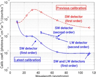
2.2 Results and comparison with a previous calibration 161

162

The method exposed in the previous section has been applied to both the 'shorter wavelength' 163

(SW) and 'longer wavelength' (LW) detectors. The brightness calibration coefficient has been 164

determined for the six wavelengths available with the calibration source. It is shown in Fig. 3. 165

As the LW detector cannot be positioned to observe wavelengths shorter than 77 Å, only the 166

coefficient at 113 Å could be obtained by this method. Interestingly, it has almost the same 167

value as for the SW detector at the same wavelength. This observation results from the fact 168

that the two detectors are practically identical. It also denotes the accuracy of the 169

interferometric alignment of the spectrometer [7] and of the mechanical positioning of the 170

detectors along the Rowland circle to better than 25 µm. In the following we will thus not 171

distinguish between the two detectors on the calibration curves. 172

173

Figure 3: Absolute brightness calibration coefficient as a function of wavelength. SW

174

detector: (red and dashed line) previous calibration in the first order and (blue and

175

solid line) latest calibration in the first and second orders. LW detector: (blue + and

dashed-176

dotted line) latest calibration in the first two orders.

177 178

8

It can be seen from the slope of the calibration curve that on the short wavelength side 179

the spectrometer sensitivity (proportional to 1/K) decreases with decreasing wavelength, 180

which illustrates the difficulty to measure spectral line intensities below 10 Å with this 181

600g/mm gold coated ruled grating. The comparison of the latest calibration curve with the 182

previous one shows that the various improvements to the spectrometer (use of two 183

microchannel plates in chevron configuration for each detector assembly, installation of a new 184

grating, better performance PDA camera) have enhanced the spectrometer sensitivity by about 185

a factor 30 over the whole calibrated wavelength range except below about 20 Å. The latter 186

feature is most likely due to the characteristics of the previous 600 l/mm holographic grating 187

which was platinum coated, while the new grating is a ruled one and gold coated with a 188

steeply decreasing efficiency toward the very short wavelengths below 15 Å.

189 190

As this new grating is not designed to suppress the higher diffraction orders, the 191

ultrasoft X- ray source lines at 44.4 Å and 67 Å have also been observed in the second order 192

and have been used for the calibration, as shown in Fig. 3. They show that the spectrometer 193

sensitivity in the second order is poorer than in the first order, but only by a factor of 5 to 8. 194

We have actually observed intense spectral lines emitted by the tokamak plasma in as high an 195

order as the 7th or the 8th. Notice that the second order calibration is almost the same for the 196

SW and the LW detectors, another indication that the two detectors are practically identical. 197

198 199

3. Sensitivity calibration in the long wavelength range 200

201

3.1 Use of the branching ratio method 202

203

The mechanical design of the spectrometer presently equipped with two detector 204

carriages sets a lower limit of about 77 Å to the spectral range accessible to the LW detector 205

(this limit is actually reached when the SW detector carriage is itself positioned at the shortest 206

possible wavelength position). The only line emitted by the ultrasoft X-ray calibration source 207

above this limit, and thus the only available one for the LW detector calibration in the first 208

order, is at 113 Å. Therefore, another method has to be used in order to calibrate the 209

spectrometer up to its maximum wavelength, which reaches 340 Å with the routinely used 210

600 g/mm grating. 211

9

The first additional method we use here is the so-called branching ratio method [1, 2], 212

which we will now describe briefly. The emissivity ratio of two spectral lines of a given ion 213

emitted by transitions from the same upper level to two different lower levels depends only on 214

atomic constants and not on the plasma conditions. In tokamak plasmas the emission is 215

completely dominated by spontaneous decay (rather than collisional de-excitation) so that the 216

ratio can be written as: 217 218 ik ij ik i ij i ik ij A A A n A n = =

ε

ε

where ni is the population density of the upper level i and Aij and Aik are the Einstein

221

coefficients for spontaneous decay from levels i to levels j and k respectively. This relation 222

holds as long as neither spectral line is self-absorbed by the plasma, i.e. when the plasma 223

optical thickness can be neglected, which is the case here since the impurity ion density is 224

always far below the main plasma ion density of about 5×1019 m-3. The effect of radiation 225

trapping on the line brightness has been calculated using a mean transmission factor approach 226

[2, 11] and the predictions were confirmed by measurements on the TA2000 torus [4]. It was 227

found that for an optical thickness of the plasma below 0.1, the self-absorption is less than 228

3.5%. It is thus negligble in the present experimental conditions. 229

Using Eq. (5) it is easy to show that the same relation can be used for the brightness 230

ratio Bij/Bik measured by a spectrometer along a line of sight through the plasma. The relation

231

between the measured signal ratio and the brightness ratio can be deduced from Eqs. 6 and 232 10: 233 234 ik ij ik ij m ik ik m ij ij A A B B N K N K = = ) ( ) (

λ

λ

This leads to the relation: 237 ik ij m ij m ik ik ij A A N N K K = ) ( ) (

λ

λ

This relation shows that the ratio of calibration coefficients at two different 240

wavelengths can be deduced from line intensity measurements, which can be performed using 241

10

the tokamak plasma itself as a calibration source, and from Einstein coefficients, which are 242

well known atomic constants in our case. This relation can thus be used for relative 243

calibration for the two wavelengths λij and λik. This is particularly useful to determine the

244

absolute calibration factor at either wavelength when it is already known at the other. As 245

already said, the latter application is often used for VUV spectrometers using a visible 246

spectrometer having the same line of sight [3,4,5]. 247

As we did not have such a setup, we took advantage of the absolute calibration over 248

the SW range described in the previous paragraph to calibrate the longer wavelength range by 249

using spectral line pairs with one line below 113 Å (measured in absolute units with the SW 250

detector) and the other at a wavelength to be calibrated above this value (measured with the 251

LW detector). This procedure relies on the assumption that the two detectors have the same 252

sensitivity at any given wavelength, an assumption supported by their identical design and by 253

the identical absolute calibration coefficient found at 113 Å in Section 2. 254

In our case, the plasma emits few pairs of lines obeying the constraints imposed by the 255

branching ratio method and the spectrometer wavelength coverage (two lines emitted from the 256

same initial level of the same ion with a sufficient intensity, the wavelength of one between 257

10 and 113 Å, the other between 113 and 340 Å). Only two suitable pairs were found, emitted 258

by Carbon, the dominant impurity in Tore Supra plasmas. They are shown in Table 3. The 259

calibration coefficients at 28.5 Å and 27.0 Å are calculated by a linear interpolation between 260

the two closest calibration points obtained in Section 2, namely 23.7 Å and 31.6 Å. 261

262

LW spectral line SW spectral line Theoretical intensity

ratio Aij/ Aik Transition λ (Å) Aij (s-1) Transition λ (Å) Aik (s-1) n=3 → n=2 (C VI) 182.2 5.72×1010 n=3 → n=1 (C VI Lyβ) 28.5 7.23×1010 0.79 n=4 → n=2 (C VI) 134.9 1.09×1010 n=4 → n=1 (C VI Lyγ) 27.0 1.66×1010 0.66 263

Table 3: Pairs of spectral lines and theoretical intensity ratios which have been used for 264

relative calibration of the spectrometer above 113 Å.

265 266

This method provides invaluable information in that it allows to link the absolute 267

calibration in the shorter wavelength range with the relative calibration in the longer 268

11

wavelength range. Nevertheless it is clearly not sufficient to calibrate the whole longer 269

wavelength range of the spectrometer coverage. A complementary method is presented below. 270

271

3.2 Collisional-radiative modelling of line intensity ratios 272

273

The results of the branching ratio method exposed in the previous paragraph do not 274

depend on the experimental conditions such as the plasma parameters and their time evolution 275

or the spectrometer line of sight geometry. However, as it has just been shown, there are in 276

general very few pairs of spectral lines which can be used in a given experimental situation. 277

Relaxing the constraint of an identical upper level for the spectral line pairs used for the 278

calibration, we find many groups of lines emitted by a given ion in the plasma within the 279

relevant wavelength range. The drawback is that the relative intensities of the lines within a 280

group depend not only on atomic physics but also on the plasma parameters. They can be 281

calculated in the frame of a collisional-radiative model (CRM). 282

This calibration method, less accurate than the branching ratio method, has been 283

applied on the SPRED VUV spectrometer at JET for the 360-980 Å range using spectral lines 284

from mostly low ionisation stages [5]. In the present work, we aimed at calibrating a shorter 285

wavelength range (130-340 Å) than at JET. We also wanted to avoid using spectral lines 286

emitted near the plasma edge, where the plasma parameters are not so well known (in 287

particular the electron temperature). For both these reasons we did not select very low 288

ionisation stages, as can be seen on Table 4. 289

290

Emitter Wavelength (Å) Transition

C IV 222.8 1s22s 2S - 1s25p 2Po 244.9 1s22s 2S - 1s24p 2Po 259.5 1s22p 2Po - 1s25d 2D 262.6 1s22p 2Po - 1s25s 2S 289.2 1s22p 2Po - 1s24d 2D 296.9 1s22p 2Po - 1s24s 2S 312.4 1s22s 2S - 1s23p 2Po C VI 27.0 1 – 4 (Ly γγγγ)))) 28.5 1 – 3 (Ly ββββ))))

12 134.9 + 135.0 2 – 4 (Balmer ββββ)))) 182.1 + 182.2 2 – 3 (Balmer αααα) O V 151.5 2s2p 3Po - 2s4d 3D 192.8 + 192.9 2s2p 3Po - 2s3d 3D O VI 129.8 + 129.9 1s22p 2Po - 1s24d 2D 150.1 1s22s 2S - 1s23p 2Po 172.9 + 173.1 1s22p 2Po - 1s23d 2D 183.9 + 184.1 1s22p 2Po - 1s23s 2S Fe XXIV 192.0 1s22s 2S - 1s22p 2Po3/2 255.1 1s22s 2S - 1s22p 2Po1/2 291

Table 4: Spectral lines used in the branching ratio method for absolute calibration transfer

292

(in bold) and in the CRM line ratio method for relative calibration.

293 294

In the collisional-radiative modelling, instead of expressing the line emissivity as a 295

function of the population density of the initial level of the transition (as in Eq. 10), we use 296

the total density nz of the emitting ion. The emissivity of a given line between levels i and j

297

can be written as: 298 299 ) , ( _{e e} ij z e ij =n n PEC n T

ε

where ne and Te are the electron density and temperature respectively. The PECij quantity,

302

called photon emission coefficient, is calculated with a collisional-radiative model (CRM). It 303

depends in a complex way on the collisional and radiative atomic processes in the plasma, 304

namely transitions between excited levels of the emitting ions, recombination onto and 305

ionisation from excited levels. The PEC dependence on ne is generally weak and will be

306

neglected here. In the present case the PEC values were obtained from the ADAS data and 307

model [12]. 308

13

From Eq. 13 it can be deduced that the emissivity ratio of two lines ij and kl emitted 309

by the same ion is equal to the PEC ratio. For the brightness, which is the quantity actually 310

measured by the spectrometer, the situation is slightly more complex: 311 312

∫

∫

where the integration is done along the line of sight. The exact calculation requires that we 315

know the spatial distribution of all quantities in the integrals, in particular the emitting ion 316

density profile along the line of sight. The most accurate way to obtain this is from a 317

dedicated transport study [13], a sophisticated and somewhat lengthy procedure. Instead, we 318

make here the rougher assumption that the PECs do not depend on Te. This is verified in our

319

case because the emitting layer of the selected ions in this study is very narrow. As an 320

additional precaution, we have rejected lines with PECs depending strongly on the 321

temperature in the Te range where the emitting ion is abundant (e.g. C V 40.3 Å, 1s2 1S0 -

322

1s2p 1P1o). As a consequence, denoting Teem the electron temperature of the emitting layer, the

323

measured brightness ratio will thus be approximately equal to the PEC ratio: 324 325 ) ( ) ( em e kl em e ij kl ij T PEC T PEC B B = (15) 326 327

An accurate determination of Teem would require either a full transport study, as

328

already mentioned, or enough lines of sight to determine experimentally the position of the 329

emission layer. The weak Te dependence requested from the PECs retained in this study

330

allowed to estimate Teem witout loss of accuracy from the position of the emitting layers as

331

calculated by a local ionisation balance calculation. 332

Denoting again Nijm the measured signal and K(

λ

333

coefficient, one gets by definition of the calibration coefficient (Eq. 6): 334 335

( )

( )

λ

λ

14

Provided the calibration coefficient is known at one wavelength, say λij, the coefficient at the

338

other wavelength λkl can be obtained by using Eq. 15:

339 340

( )

( )

Comparing the calculated and measured C VI line brightness ratios, we have 343

calculated the absolute calibration coefficients at 134.9 Å and 182.2 Å. Note that at 134.9 Å 344

the Balmer β line is blended with the fourth order of the C VI Ly α line at 33.7 Å. In order to 345

subtract the latter contribution it was necessary to estimate the grating efficiency in the fourth 346

order. This was done by measuring the intensity of the well resolved C V 34.97 Å line in the 347

first and fourth orders in identical pulses designed for the calibration described here (see next 348

Section). This allowed us to deduce that the grating efficiency in the fourth order with respect 349

to that in the first order is about 10% at this wavelength. The contribution of the fourth order 350

C VI Ly α line to the measured 134.9 Å intensity was then calculated using the measured first 351

order C VI Ly α line intensity and the fourth order efficiency. It was then subtracted from the 352

measured intensity at 134.9 Å before the calibration coefficients were calculated. 353

Then we interpolate the calibration coefficient of the 150.1 Å line of the O VI group 354

between the values at 134.9 Å and 182.2 Å. From there, we use Eq. 17 with the O VI line 355

group to obtain the calibration coefficients at 129.9 Å, 173 Å and 184 Å. Then with the same 356

hypothesis we obtain the 151.5 Å (O V group) calibration coefficient, and this allows us to 357

obtain the calibration coefficient at the second wavelength of the O V group, 192.9 Å. With 358

the same reasoning, we obtain the calibration coefficients at 192.0 Å and 255.1 Å (Fe XXIV 359

group) and at the six wavelengths of the C IV group. It has been checked that the final result 360

(the curve which will be fitted to the data points) remains within the error bars if the order in 361

which the line groups are added is changed. 362

363

4. Results and uncertainties 364

365

4.1. Results 366

367

A series of identical, ohmic pulses have been performed to record the useful spectral 368

line brightnesses (Tore Supra pulses TS#31512 to TS#31519). The plasmas are found to be 369

15

very stationary and reproducible so there was no need to perform a multi-pulse statistical 370

study of the line ratios. The spectrometer was used in its spatial scanning mode, which means 371

that the whole spectrometer was rotated around a horizontal axis located in front of the 372

apparatus. In this mode of operation, the lower half of the plasma (see Fig. 4) could be 373

scanned at a period of 0.5 Hz. 374

375

Figure 4: Poloidal cross section (solid line) of the tokamak vessel, (dashed-dotted 376

line) of the plasma last closed flux surface and (dashed line) of the extreme positions of the

377

line of sight.

378 379

Both the spectral line shapes and the radial profiles were used to reject blended lines. 380

In the case of the Fe XXIV lines, observed to be blended in [5], the analysis of the radial 381

brightness profiles allows to distinguish them from blended light species lines. 382

The calibration coefficients obtained with this method have been added to the results 383

obtained in Section 2.2. The overall calibration curve is shown in Fig. 5. It shows a broad 384

minimum (corresponding to a maximum in sensitivity) around 100 Å over a range of about 70 385

Å. The spectrometer sensitivity decreases steeply on both sides, although in the long 386

wavelength direction the slope tends to become lower. This indicates that with the same 387

grating a modified spectrometer with a longer mechanical range for the detector would be 388

sensitive enough to provide information over a broader wavelength range. This has been done 389

for the Schwob-Fraenkel spectrometer installed on the Berlin EBIT experiment [14, 15]. On 390

the contrary, in the short wavelength direction the slope is steeper and steeper. This indicates 391

that extending the mechanical range to shorter wavelengths would not provide additional 392

useful information below 10 Å. 393

16 395

Figure 5: Absolute brightness calibration in lab (solid line with ), calibration transfer using 396

the branching ratio method ( ) and relative calibration using the CRM of line ratios with

397

plasma (the symbols are explained on the figure). The grey dashed line is a spline among the

398

points and is adopted as the final calibration curve.

399 400

4.2. Uncertainties 401

402

In the wavelength range absolutely calibrated with the ultrasoft-X ray source (9.9 - 403

113 Å), the main uncertainty is that associated with the spectral line intensities measured with 404

the spectrometer. It is mostly due to the uncertainty on the background estimate, which can be 405

difficult for the weaker lines of the calibration source. The uncertainty on these intensities is 406

at maximum 10% (it can be as low as 5% for the stronger lines). In addition, we estimate an 407

uncertainty of 10% to take account of the geometric aperture uncertainty. The uncertainty on 408

the proportional gas counter measurements is negligible compared to those associated with 409

the spectrometer measurements. We have thus a global uncertainty of 20% for the calibration 410

coefficients up to 113 Å. 411

For the calibration points using the branching ratio method, we must take into account 412

the time fluctuations of the two spectral line intensities used for each point. These fluctuations 413

are not negligible even during the stationary phase of the plasma. They are actually much 414

larger than the statistical error (which is the square root of the time average signal if a Poisson 415

distribution is assumed). The total uncertainty is thus estimated to 40% at 134.9 Å and 32% at 416

182.2 Å. 417

17

For the CRM calibration method, a part of the uncertainty associated with the 418

reference line (at wavelength λ0) of a given line group is determined from the time fluctuation

419

of the measured signal as discussed in the previous paragraph. To this fluctuation uncertainty, 420

an uncertainty of 30% is added, corresponding to the interpolation of this reference line 421

between two already calibrated wavelengths. For any other line (wavelength λ) of the group, 422

the uncertainty is deduced from Eq. 17: 423 424 ) ( ) ( ) ( ) ( ) ( ) ( ) ( ) ( ) ( ) ( ) ( ) ( 0 0 0 0 0 0 λλ λλ λλ λλ λλ λλ m m m m N N N N PEC PEC PEC PEC K K K K ₊∆ ₊∆     ∆ + ∆ = ∆ (18) 425 426

The relative uncertainties on the signals Nm(

λ

λ

427

fluctuations of the measurements, as said above. The uncertainty on the PECs themselves is 428

difficult to assess and not always available in the literature. It seems that a global value of 429

30% for all PEC ratios reflects satisfactorily both the accuracy of the atomic physics 430

calculations and the residual PEC ratio dependence on (see above the discussion about

431

Eq. 15) . 432

433

For a practical purpose, a curve has been fitted on the points in Fig. 5. The most 434

satisfactory result was obtained with a spline. Below 120 Å the 20% uncertainty estimated for 435

the absolute calibration points can be retained. Between 120 and 180 Å, where line intensity 436

branching ratios were available, an uncertainty of about 35% is estimated. Above this 437

wavelength, a value of 50% reflects satisfactorily the spreading and uncertainties of the 438

relative calibration points. In this range, the uncertainty might be an underestimate of the 439

actual uncertainty due to the use of the CRM, for which the uncertainties are not well known. 440

441 442 443

5. Spatial variations of the detector response 444

445

The tolerances of the spectrometer design and realisation are very tight, so that most 446

mechanical pieces are positioned to less than 25 µm. Nevertheless, the response of the 447

detector assembly along its length (i. e. along the wavelength direction) is not perfectly 448

18

uniform. It can be due to several reasons such as the small inhomogeneities of the 449

multichannel plate and phosphor screen responses, the transmission of the fiber optics bundle 450

or the quantum efficiency dependence on the photon incidence angle on the MCP input face. 451

As the non-uniformity and the spatial variation of the detector response play a role in 452

the estimate of the spectral line absolute brigthnesses, it has been measured for the LW 453

assembly. The simplest way of doing this measurement is to select a spectral range containing 454

well isolated spectral lines and perform several measurements, moving the detector by small 455

position shifts between measurements in such a way that the spectral lines would strike 456

different parts of the MCP. 457

Due to programme constraints, this method could not be applied in the spectroscopy 458

laboratory. Therefore we have used the same series of identical discharges on the Tore Supra 459

tokamak as for the calibration. During this series, the detectors were moved in a limited 460

number of positions. As a result of this procedure, many spectral lines could be measured at a 461

few positions on the detector. By comparing the spectrometer measurements of a given 462

spectral line in the various positions and synthetising the results for all lines, we were able to 463

deduce the non-uniformity and spatial variation of the detector assembly response. The list of 464

the lines used for this procedure is given in Table 5. 465 466 Wavelength (Å) Emitter 129.9 O VI 132.9 Fe XXIII 134.9 C VI 2-4 (+ Ly α 4th order) 135.8 Fe XXII 238.5 O IV, C IV 241.5 C V (40.3 Å 6th order) 244.9 C IV 281.9 C V 284.1 Fe XV 289.2 C IV 292.0, 291.3 Ni XVIII, C III 467

Table 5: List of spectral lines and corresponding emitters for the evaluation of the non-468

uniformity and spatial variation of the detector response.

19 470

The synthesis of all these measurements is presented on Fig. 6. The results show that 471

the intensity response is a decreasing function of the spectral line position in the direction of 472

increasing pixel number (corresponding to increasing wavelengths) on the MCP detector in 473

the useful range (between pixels 70 and 900 for the LW detector). The measurements show 474

that the response at both ends of the detector (below pixel 70 and above pixel 900) is 475

substantially degraded with respect to the major part of the detector range. This is due to the 476

fact that the size of the PDA is slightly larger than the fiber optics bundle size. One notices 477

that the unuseful portion on the large pixel number extremity is wider than that on the small 478

pixel number extremity. This indicates that the bundle is not perfectly centred on the 479

photodiode array. Both ends of the detector have thus been excluded from the study. 480

A straight line has been fitted to the data and the correction factor curve thus obtained 481

has been normalised so that it is 1 in the middle of the detector (pixel 512 here). The 482

spreading of the points around a given position and wavelength in Fig. 6 indicates that the 483

measurement fluctuations are dominant over the spatial inhomogeneities along the detector. 484

The response decrease along the detector seems to be mostly related to the varying response 485

of the MCP with the photon incidence angle. Indeed it is known that the MCP quantum 486

efficiency decreases as the incoming photon angle with the grating plane becomes more 487

grazing. 488

In Fig. 6, the average slope for the group of lines around 130 Å does not show a 489

significant difference with that for the group in the range 240-292 Å (it would correspond to a 490

response difference of less than 3%). Therefore we can consider that the wavelength 491

dependence of the detector response spatial variation can be neglected. As no data in the short 492

(10-70 Å) wavelength range are available for this calibration campaign, the average decrease 493

of Fig. 6 was used to correct all the line intensity measurements performed for the Manson 494

source and the branching ratio methods (Figure 5 includes these corrections.) As the intensity 495

response curve introduces a maximum correction of about 20%, which is small compared 496

with the global uncertainty estimated in Section 4.2, it was not necessary to make this 497

correction for the CRM calibration above 200 Å. 498

20 500

Figure 6: Intensity response of the LW detector assembly as a function of the line position on 501

the detector (measured in pixels). Each symbol represents a different spectral line (see list on

502

Table 4). Dashed line: final correction factor.

503 504

6. Summary and conclusion 505

The grazing incidence spectrometer operated on Tore Supra with a 600g/mm grating 506

blazed at 1.5° has been absolutely calibrated over most of its wavelength coverage, i. e. 9.9-507

312 Å. For the lower part of this domain (9.9-113 Å) we have used an ultrasoft-X ray source 508

calibrated against a gas flow proportional counter set up with a 100% efficiency. For the rest 509

of the wavelength domain we have used the branching ratio method for absolute calibration 510

transfer and collisional-radiative modelling of line intensity ratios for relative calibration. 511

The results show that the spectrometer sensitivity has improved with respect to the 512

previous setup thanks to the new grating and the double multichannel plates in chevron 513

configuration. The spectrometer is most sensitive in the 50-200 Å range, with a steep decrease 514

below 50 Å. On the long wavelength side the sensitivity decrease is not as steep. In fact, after 515

the present calibration procedure we have exchanged the 600 g/mm grating with a 300 g/mm 516

one and obtained useful measurements up to 680 Å. 517

The uncertainties have been calculated for each individual calibration wavelength. Due 518

to the variety of methods used for the whole wavelength range, it is not straightforward to 519

determine a precise global uncertainty. We estimate a 20% uncertainty below 120 Å, where 520

direct absolute calibration was obtained with the ultrasoft-X ray source, and 35% in the range 521

120-180 Å where the line branching ratio method was used. In the range above 180 Å where 522

only the relative calibration procedure (collisional-radiative modelling of line intensity ratios) 523

21

was available, the uncertainty is estimated to 50% or even more. This reflects the larger 524

uncertainties and the spreading of the individual calibration points in the LW range. 525 526 527 528 Bibliography 529 530

[1] E. Hinnov and W. Hofmann, J. Opt. Soc. Am. 53 (1963) 1259 531

[2] J.L. Schwob and C. Breton, C. R. Acad. Sc. 261 (1965) 1476 532

[3] J.L. Schwob, C. R. Acad. Sc. 262 (1966) 1264 533

[4] J.L. Schwob, CEA report R-3359 (1969) 534

[5] K. Lawson, I. Coffey, J. Zacks, M.F. Stamp and JET-EFDA contributors, J. Instr. 4 (2009) 535

P04013 536

[6] J. Park, G.V. Brown, M.B. Schneider, H.A. Baldis, K.V. Cone, R.L. Kelley, C.A. 537

Kilbourne, E.W. Magee, M.J. May and F.S. Porter, Rev. Sci. Instrum. 81 (2010) 10E319 538

[7] J.L. Schwob, A.W. Wouters, S. Suckewer and M. Finkenthal, Rev. Sci. Instrum. 58 (9) 539

(1987) 1601 540

[8] R. Prakash, J. Jain, V. Kumar, R. Manchanda, B. Agarwal, M.B. Chowduri, S. Banerjee 541

and P. Vasu, J. Phys. B 43 (2010) 144012 542

[9] J.E. Manson, Manson model 5 ultrasoft-X ray calibration source,1985; Austin Instruments 543

Inc. 544

[10] D. Stutman, S. Kovnovich, M. Finkenthal, A. Zwicker and H.W. Moos, Rev. Sci. 545

Instrum. 62 (1991) 2719 546

[11] C. Breton and J. L. Schwob, C. R. Acad. Sc. 260 (1965) 461 547

[12] H. P. Summers, Atomic Data and Analysis Structure User Manual

548

(2007) http://www.adas.ac.uk/

549

[13] D. Villegas, R. Guirlet, C. Bourdelle, X. Garbet, G.T. Hoang, R. Sabot, F. Imbeaux and 550

J.L. Ségui, Nucl. Fusion 54 (2014) 073011 551

[14] C. Biedermann, R. Radtke, J.L. Schwob, P. Mandelbaum, R. Doron, T. Fuchs and G. 552

Fussmann, Physica Scripta T92 (2001) 85 553

[15] R. Radtke, C. Biedermann, J.L. Schwob, P. Mandelbaum and R. Doron, Phys. Rev. A 64 554

(2001) 012720 555