Radiative Decay Parameters for Highly Excited Levels in
Ti II
H. Lundberg,
1
?
H. Hartman,
2,3
L. Engstr¨
om
1
H. Nilsson
3
A. Persson
1
P. Palmeri
4
P. Quinet
4,5
V. Fivet
4
G. Malcheva
6
and K. Blagoev
6
1Department of Physics, Lund University, P.O. Box 118, S-221 00 Lund, Sweden, Lund 2Applied Mathematics and Material Science, Malm¨o University, 20506 Malm¨o, Sweden
3Department of Astronomy and Theoretical Physics, Lund University, P.O. Box 43, S-221 00 Lund, Sweden 4Physique Atomique et Astrophysique, Universit´e de Mons, B-7000 Mons, Belgium
5IPNAS, Universit´e de Li`ege, B-4000 Li`ege, Belgium
6Institute of Solid State Physics, Bulgarian Academy of Sciences, 72 Tzarigradsko Chaussee, BG - 1784 Sofia, Bulgaria
Accepted XXX. Received YYY; in original form ZZZ
ABSTRACT
The present work reports new experimental radiative lifetimes of six 3d2(3F)5s levels in singly ionized titanium, with an energy around 63000 cm−1 and four 3d2(3F)4p odd parity levels where we confirm previous investigations. Combining the new 5s lifetimes with branching fractions measured previously by Pickering et al. [Astrophys Journal Suppl Ser 132, 403 (2001)], we report 57 experimental log g f values for transitions from the 5s levels. The lifetime measurements are performed using time-resolved laser-induced fluorescence on ions produced by laser ablation. One- and two-step photon excitation is employed to reach the 4p and 5s levels, respectively. Theoretical calculations of the radiative lifetimes of the measured levels as well as of oscillator strengths for 3336 transitions from these levels are reported. The calculations are carried out by a pseudo-relativistic Hartree-Fock method taking into account core polarization effects. The theoretical results are in a good agreement with the experiments and are needed for accurate abundance determinations in astronomical objects.
Key words: atomic data – methods: laboratory: atomic
1 INTRODUCTION
Lines from the iron-group elements are among the most abundant in spectra of astronomical objects. In the B, A and F class stars, the first ions of Fe, Cr and Ti dominate the ultraviolet and visible spectrum. Even so-called forbid-den lines in Ti II have been found to be very intense in the strontium filament ejecta of the massive star Eta Carinae (Hartman et al. 2004). Titanium is located among the lighter of the iron group elements and is considered primarily to be an α-element, i.e. produced by successive captures of He nu-clei through among others, Mg, Si and Ca. Recent studies of metal poor stars, however, show trends where the tita-nium abundance is correlated with scandium and vanadium indicating a similar production mechanism as the iron-group
elements rather than the α-elements (Sneden et al. 2015).
Accurate atomic data are needed to reliably determine the Ti abundance in these objects.
? E-mail: [email protected]
The ground term in Ti ii is 3d24s4F, followed by even
terms belonging to the 3d24s, 3d3 and 3d4s2 configurations
up to an energy of 25000 cm−1. The lowest odd
configu-rations are 3d24p and 3d4s4p spanning the energy
inter-val from 29500 to 59500 cm−1 (Huldt et al. 1982).
Tran-sitions between these configurations give rise to the most intense spectral lines in Ti ii, and have been the subject of most previous experimental and theoretical investigations.
The higher lying even configurations 3d25s, 3d26s, 3d24d
and 3d25d cover the energy interval from 62180 cm−1 to
84652 cm−1. In total 253 energy levels and 1872 spectral
lines ranging from 122 to 2198 nm are reported in the NIST
compilations (Kramida et al. 2014;Saloman 2012).
Experimental lifetimes in Ti ii obtained with different techniques have been reported in several papers. The first
investigation, byRoberts et al. (1973), used the beam-foil
method to obtain lifetimes in both the 4p and 4d
configu-rations. InGosselin et al.(1987) a Ti+ beam from a heavy
ion accelerator was crossed by a laser to selectively excite the 4p z4D
uncer-tainty of only 1.5 % and remains the most accurately known
lifetime in Ti ii.Langhans et al.(1995),Kwiatkowski et al.
(1985) and Bizzarri et al. (1993) employed time-resolved
laser-induced fluorescence (TR-LIF) on ions from a
hol-low cathode discharge. The metastable states of the 3d3,
3d2(3P)4s and (3d + 4s)3electron configurations of Ti ii have been investigated by a laser probing technique on Ti ions
in a storage ring in series of papers (Hartman et al. 2003;
Palmeri et al. 2008; Hartman et al. 2005). Along with the lifetimes, transition probabilities for several decay channels from these metastable levels are also reported.
A number of experimental investigations of both ab-solute and relative transition probabilities and oscillator strengths from 4p levels have been stimulated by astro-physical observations. Various methods and spectral sources have been employed. These include absorption
measure-ments (Wiese et al. 2001), emission studies from a shock
tube (Boni 1968;Wolnik & Berthel 1973), from arc- (Tatum 1961;Roberts et al. 1975) and spark-sources (Wobig 1962),
hook method (Danzmann & Kock 1980) and Fourier
trans-form spectroscopy (Pickering et al. 2001;Wood et al. 2013).
Several papers report theoretical investigations of
radia-tive parameters in Ti ii. The most recent of these areKurucz
(2011) and Ruczkowski et al. (2014). Transition
probabili-ties and oscillator strengths of Ti ii spectral lines are also
included in several compilations, e.g. Th´evenin (1989),
Sa-vanov et al.(1990) andMeylan et al.(1993).
This short literature survey shows that a large number of studies have been devoted to transition probabilities and radiative lifetimes for low lying excited states, mainly
be-longing to the 3d24p electron configuration. There are no
experimental data for the high lying 5s levels that are the main subject of the present work.
2 EXPERIMENT
The experimental set-up for single-step experiments at the Lund High Power Laser Facility has recently been described
in detail (Engstr¨om et al. 2014), and here we focus mainly
on the new features involved in the two-step process. The
experimental set-up is presented in Fig. 1. The Ti ions are
produced in an ablation process, where the second harmonic of a Nd:YAG laser (Continuum Surelite) with 10 ns pulses are focused on a rotating Ti target. The target is placed in
a vacuum chamber with a pressure of around 10−4 mbar.
The generated plasma is crossed by the two excitation laser beams about 1 cm above the target. With the first laser the
intermediate odd states in 3d2(3F)4p, around 32000 cm−1,
are excited and used as platforms for the excitation of the high-lying even parity 5s states.
The first laser channel consist of a Nd:YAG laser (Con-tinuum NY-82) pumping a Con(Con-tinuum Nd - 60 dye laser
op-erating with DCM dye (C19H17N3O). The 10 ns long pulses
are frequency doubled using a KDP crystal (KH2PO4). For
the second step, the same type of lasers and dye are used but here the Nd:YAG laser is injection seeded and the pulses are temporally compressed using stimulated Brillouin scattering (SBS) in water. After frequency doubling in a KDP crystal we obtain pulses with a typical FWHM of 1.2 ns.
All three laser systems operate at 10 Hz and are syn-chronized by a delay generator. The delay generator allows
Delay Unit Nd:YAG Laser Nd:YAG Laser Seeded SBS Compressor Dye Laser KDP BBO Trigger
Nd:YAG Laser DyeLaser KDP BBO Detection area Rotating target Monochromator MCP PMT Oscilloscope Computer
Figure 1. Experimental set-up for TR-LIF at the Lund High Power Laser Facility using two-step excitation. See discussion in text for details.
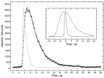
Figure 2. The first 30 ns of the decay of the e2F
5/2level in Ti ii following two-step excitation. The measured decay (+) is plotted together with a fitted single exponential function (solid line) con-voluted by the recorded second step laser pulse (dashed curve). The insert shows the timing between the fluorescence from the intermediate z2D3/2 level (broad structure) and the second step laser (narrow peak).
us to set the time between the plasma generating laser and the excitation pulses (typically around 1 µs) and also the delay between the first and second excitation steps. The lat-ter timing was checked before every measurement to ensure that the second step occurred at the maximum population of the intermediate level, as determined by the decay of this level in some channel. Since the pulses in the first step are much longer than in the second step this also ensures that the intermediate population is almost constant during the final excitation. The timing between the two steps is illus-trated in the insert in Fig.2.
The fluorescence from the excited states was observed with a 1/8 m grating monochromator, with its 0.28 mm wide entrance slit oriented parallel to the excitation lasers, giv-ing a line width of 0.5 nm in the second spectral order. The
0 10000 20000 30000 40000 50000 60000 70000
Ener
gy
(cm
-1)
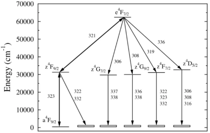
e4F7/2 z4F9/2 a4F9/2 z4G9/2 z4G7/2 z 4 F7/2 z 4 D5/2 323 322 332 337 338 336 338 322 323 332 306 308 316 321 308 306 319 336Figure 3. Decay chains from the 5s e4F
7/2level in Ti ii. All wave-lengths are given in nm. In the experiment the 5s level is excited in two steps using the transitions at 323.4 nm (4s - 4p) and 321.3 nm (4p - 5s).
dispersed light was registered by a fast micro-channel-plate photomultiplier tube (Hamamatsu R3809U) and digitized by a Tektronix DPO 7254 oscilloscope triggered by the sec-ond step laser pulses detected with a fast photodiode. The final decay curves and pulse shape were obtained by
averag-ing over 1000 laser pulses. The code DECFIT (Palmeri et al.
2008) was then used to extract the lifetimes by fitting a
sin-gle exponential function convoluted by the measured shape of the second step laser pulse and a background function to
the observed decay. A typical example is shown in Fig.2.
Table 1 gives the wavelengths and excitation schemes
used in the single-step measurements of four 4p levels, per-formed to allow a comparison with earlier experimental re-sults. Two of these levels are also used as platforms in the two-step experiments. A complete description of the latter
is given in Table2. In the complex level system of the iron
group elements, with a parent term structure and multiple ionization limits, the strong transitions group in wavelengths due to the similar energy difference between 4s and 4p for the different parent terms (similar promotion energy). In ad-dition, the energy difference between 4p and 5s is similar to that of 4s and 4p, making the transitions between these con-figurations also fall in the same region. For Ti ii this region is between 300 and 350 nm. Thus, the observed decay from the 5s levels under investigation might be blended with
flu-orescence from 4p levels. Fig.3presents a schematic picture
using 5s e4F
7/2 as an example. Two types of blending may
be distinguished: from a direct fluorescence (4s - 4p) channel from the intermediate level or from the secondary decay of a 4p level populated by the decay from the 5s level studied. While the fluorescence from the intermediate level is very intense and observable even at a rather large wave-length off-set its perturbing influence is easily handled by recording an additional decay curve, with the second step laser turned off to reveal the blending contribution, which can be subtracted from the primary decay measurement be-fore the lifetime analysis. Two examples of this problem were
encountered and are marked in Table2. Secondary decays,
on the other hand, arise from decays along a chain from the level of interest and cannot be corrected for, but must be understood in order to choose an appropriate channel for the primary decay measurement. For example, the lifetime of 5s e4F
7/2 is measured in the channel 319 nm, with the
final result of (3.02 ± 0.20) ns, after correction for the first step fluorescence at 323 nm. However, the decay could be observed in three other sufficiently intense channels as well: 306, 308 and 336 nm. These are, however, blended by one or
more secondary decays, as shown in Fig.3. The measured
lifetimes in these channels are 6.5, 3.8 and 3.3 ns, respec-tively, clearly demonstrating the importance of choosing an appropriate decay channel.
The final lifetimes obtained are presented in Table 3.
The values represent the average of between 10 and 20 mea-surements performed over a number of days, and the quoted uncertainties take into account both the statistical uncer-tainty in the fitting process and, primarily, the variation of the results between the different measurements.
In Table 4 we have derived absolute transition
probabilities and log g f values for 57 transitions de-population 5 of the 6 5s levels investigated in this work. The results are obtained by combining our
experimental lifetimes in Table 3 with
experimen-tal branching fractions reported by Pickering et al (2001).
3 THEORY
The relativistic Hartree-Fock (HFR) approach (Cowan 1981)
including core-polarization (CPOL) effects by means of a model potential and a correction to the transition dipole
operator (HFR + CPOL) (see e.g.Quinet et al. 1999 and
Quinet et al. 2002) has been used to compute the transition probabilities in Ti ii. The following 27 configurations have been considered explicitly in our physical model: 3d3, 3d24s, 3d25s, 3d26s, 3d24d, 3d25d, 3d4s2, 3d4p2, 3d4d2, 3d4s4d, 3d4s5d, 3d4s5s, 4s24d, 4s25d, 4s25s (even parity) and 3d24p, 3d25p, 3d24f, 3d25f, 3d4s4p, 3d4s5p, 3d4s4f, 3d4s5f, 4s24p,
4s25p, 4s24f, 4s25f (odd parity). The ionic core considered for the core-polarization effects was an argon-like core, i.e. a 3p6 Ti V core. The dipole polarizability, αd, for such a core
is 1.48 a3
0, according toJohnson et al.(1983). For the cut-off
radius, we used the HFR mean value of the outermost 3p core orbital, i.e. 1.08 a0.
Radial integrals of the 3d3, 3d24s, 3d25s, 3d24d, 3d4s2,
3d24p and 3d4s4p, considered as free parameters, were then
adjusted with a well-established least-squares optimization program minimizing the discrepancies between the calcu-lated Hamiltonian eigenvalues and the experimental energy
levels taken from Huldt et al. (1982). More precisely, the
average energies (Eav), the electrostatic direct (Fk) and
ex-change (Gk) integrals, the spin-orbit (ζnl) and effective
in-teraction parameters (α and β ) were allowed to vary during
the fitting process. We also adjusted the CI parameters (Rk)
between the 3d3and 3d24s even configurations and between
the 3d24p and 3d4s4p odd configurations. For parameters
belonging to other configurations, a scaling factor of 0.80 was applied.
The numerical values of the parameters adopted in
Table 1. Single-step excitation schemes for 3d2(3F)4p levels in Ti ii.
Level Ea/cm−1 Starting level Excitationb λc obs/nm Ea/cm−1 λ air/nm z4F 5/2 30958 0 322.92 333 z2D 3/2 31756 0 314.80 368 z4D 5/2 32698 1087 316.26 307, 308, 316 z4D 7/2 32767 393 308.80 217 aHuldt et al.(1982).
bAll levels were excited using the second harmonic of the dye laser.
cAll fluorescence measurements were performed in the second spectral order.
for even and odd-parity configurations, respectively. This semi-empirical process led to average deviations with
exper-imental energy levels equal to 125 cm−1 (even parity) and
78 cm−1 (odd parity).
4 RESULTS AND DISCUSSION
Table3shows that our lifetimes for the 4p levels agree with
the previous investigations using laser excitation within the mutual error bars. Although there is a tendency for the new results to be somewhat shorter. Compared with the old
val-ues obtained by the beam-foil technique by Roberts et al.
(1973) we note a significant discrepancy. This is most likely
caused by the combined problem of line blending and cas-cades from higher lying states caused by the non-selective
excitation in the beam-foil process. In the case of the 3d25s
e2F7/2level,Roberts et al.(1973) measured the lifetime
us-ing a transition at 348.4 nm, but assigned the value to the configuration 3d4s4p. This is most likely a typographical er-ror since e2F denotes an even configuration. The line at 348.4
nm is an intense transition used in the present work to mea-sure the 5s e2F7/2level (Table2) and we believe that the
as-signment by Roberts et al. (1973) should be changed.
Doing so also results in agreement between the measured lifetimes.
The computed radiative lifetimes obtained in the present work are compared with our experimental values
in Table 3. As shown in this table, the overall agreement
between theory and experiment is very good (within 10%).
For comparison, Table 3 includes the theoretical lifetimes
obtained by Kurucz (2011). This work also used a
semi-empirical approach based on a superposition of
configu-rations calculation with a modified version of the Cowan
(1981) codes and experimental level energies. We note a very
good qualitative agreement between the two calculations.
Table 7 gives the HFR+CPOL oscillator strengths
(log g f ) and weighted transition probabilities (gA), obtained in the present work, for 3336 Ti ii spectral lines from 138
to 9966 nm, combining lower levels in the range 0
– 74000 cm−1 and upper levels 30000 – 80000 cm−1.
Only transitions with log g f > -4 are reported in the table in which we also give, in the last column, the value of the
can-cellation factor (CF), as defined byCowan(1981). Very small
values of this factor (typically < 0.05) indicate strong can-cellation effects in the calculation of the line strengths and the corresponding transition rates can be affected by larger uncertainties and should be considered with some care.
Table 2. Two-step excitation schemes for 3d2(3F)5s levels in Ti ii. Final Ea/cm−1 Intermediate Excitationb λc
obs/nm level level Ea/cm−1 λ air/nm e4F 3/2 62180 30958 320.20 306, 319 e4F 5/2 62272 30958 319.26 305, 318d e4F 7/2 62411 31301 321.35 319e e4F9/2 62595 31301 319.46 306 e2F 5/2 63169 31756 318.25 312, 349 e2F 7/2 63446 32025, 32767 318.17, 325.86 313f, 348 aHuldt et al.(1982).
bAll levels were excited using the second harmonic of the dye laser.
cAll fluorescence measurements were performed in the second spectral order.
dCorrected for scattered light from the second step laser at 319 nm.
eCorrected for fluorescence background from first step laser at 323 nm.
fCorrected for fluorescence background from first step laser at 316 nm.
Table 3. Lifetimes of the 3d2(3F)4p and 5s levels in Ti ii.
Level Ea τ
exp/ns τcalc/ns cm−1 Our work Other Our work Kuruczb 4p z4F 5/2 30958 3.87 ± 0.20 4.1 ± 0.2c 3.76 4.15 4.1 ± 0.3d 4p z2D 3/2 31756 6.10 ± 0.20 6.6 ± 0.3c 5.87 6.85 6.3 ± 1d 7.8 ± 1e 4p z4D 5/2 32698 3.86 ± 0.20 4.0 ± 0.2c 3.47 3.92 3.9 ± 0.4d 5.2 ± 0.8e 4.01 ± 0.06f 4p z4D 7/2 32767 3.75 ± 0.20 4.0 ± 0.2c 3.40 3.85 4.1 ± 0.5d 5s e4F3/2 62180 2.96 ± 0.20 3.19 2.82 5s e4F 5/2 62272 3.05 ± 0.20 3.19 2.82 5s e4F 7/2 62411 3.02 ± 0.20 3.19 2.82 5s e4F 9/2 62595 3.14 ± 0.20 3.19 2.82 5s e2F 5/2 63169 3.04 ± 0.15 3.41 3.04 5s e2F 7/2 63446 3.02 ± 0.15 3.0 ± 0.6e1 3.41 3.05 aHuldt et al.(1982). bKurucz(2011).
cBizzarri et al.(1993), TR-LIF. dKwiatkowski et al.(1985), TR-LIF. eRoberts et al.(1973), Beam-Foil.
e1The original assignment of this level inRoberts et al.(1973) to 3d4s(3F)4p is changed to 3d2(3F)5s.
fGosselin et al.(1987), Beam-Laser.
In the same table, we list the most recent
oscilla-tor strengths published by Pickering et al. (2001), Kurucz
(2011), Wood et al. (2013) and Ruczkowski et al. (2014).
In the work of Pickering et al.(2001), the relative
intensi-ties of Ti ii emission lines between 187 and 602 nm from 89 levels were measured by high-resolution Fourier transform spectrometry, using a hollow cathode lamp as light source. The branching fractions were then combined with 39 mea-sured and 44 computed lifetimes to give absolute transition
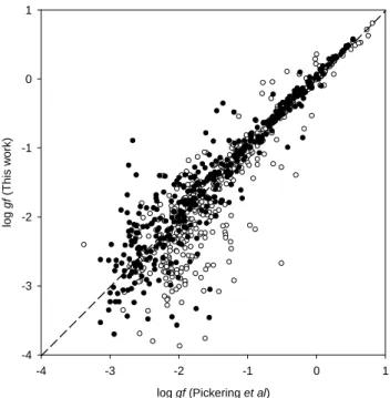
probabilities for 624 lines. Fig.4shows the good agreement
between our calculated logg f values and the values from
Pickering et al.(2001), particularly when they used
log gf (Pickering et al) -4 -3 -2 -1 0 1 lo g g f (T h is w o rk ) -4 -3 -2 -1 0 1
Figure 4. Comparison between the oscillator strengths (log g f ) calculated in the present work and those published by Picker-ing et al.(2001). The circles correspond to the combina-tion of measured branching fraccombina-tions with experimental (black) and theoretical (white) lifetimes inPickering et al.(2001).
detailed comparison between our calculated log g f values and those obtained by combining the new
ex-perimental lifetimes in Table 3 with the branching
fractions measured by Pickering et al (2001). A very good agreement is observed, in particular for the strongest transitions for which both sets of results agree within 10-20%. The average deviation in the log g f values is 0.1 with a standard deviation of 0.3.
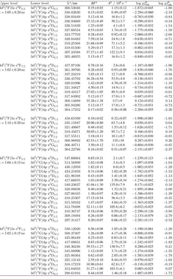
In the analysis of Wood et al. (2013), atomic
transi-tion probability measurements for 364 lines in the UV to near-IR are reported. They were obtained from branching fraction measurements using a Fourier transform spectrom-eter and an echelle spectromspectrom-eter combined with published radiative lifetimes. A comparison between these values and
our calculated log g f values is shown in Fig.5, and we note
again the consistency between the calculated and observed values.
Kurucz(2011) used a similar semi-empirical HFR model as the one considered in our work but without inclusion of
core-polarization effects. More recently, Ruczkowski et al.
(2014) used a semi-empirical oscillator strength
parametriza-tion method to compute 1340 log g f values for spectral lines in Ti ii. As seen in Table7, our new g f -values are in rather good agreement with these last results, in particular for the strongest lines (log g f > -1), for which the typical average deviations are found to be within 20%.
log gf (Wood et al)
-4 -3 -2 -1 0 1 lo g g f (T h is w o rk ) -4 -3 -2 -1 0 1
Figure 5. Comparison between the oscillator strengths (log g f ) calculated in the present work and those published byWood et al.(2013).
5 CONCLUSIONS
We report new experimental radiative lifetimes of ten 4p and 5s levels in singly ionized titanium. The measurements are performed using time-resolved laser-induced fluorescence on ions produced by laser ablation. One- and two-step photon excitation is employed to reach the 4p and 5s levels, respec-tively. For 5 of the 6 measured 5s levels we have com-bined our lifetimes with the experimental
branch-ing fractions measured previously byPickering et al.
(2001) to obtain 57 experimental absolut transition
probabilities and log g f values. In addition, we report calculated transition probabilities for 3336 Ti ii spectral lines from 138 to 9966 nm. Where possible to compare, we find a good agreement with previous experiments and calculations. The transition probabilities are needed for accurate abundance determinations in astronomical objects.
ACKNOWLEDGEMENTS
This work has received funding from LASERLAB-EUROPE (grant agreement no. 284464, EC’s Seventh Framework Pro-gramme), the Swedish Research Council through the Lin-naeus grant to the Lund Laser Centre and a project grant 621-2011-4206, and the Knut and Alice Wallenberg Founda-tion. P.P. and P.Q. are respectively Research Associate and Research Director of the Belgian National Fund for Scien-tific Research F.R.S.-FNRS from which financial support is gratefully acknowledged. V.F, P.P., P.Q., G.M. and K.B. are grateful to the colleagues from Lund Laser Center for their kind hospitality and support. We thank the anonymous ref-eree for careful reading of the manuscript and valuable sug-gestions.
Table 4. Transition probabilities and oscillator strengths for lines from the 5s levels measured in this work. Upper level Lower level λa/nm BFa Ab / 106s−1 log g fb
exp log g fcalcb 3d2(3F)5s e4F 5/2 3d2(3F)4p z2G5/2 360.53046 0.35±0.03 1.15±0.12 −1.872±0.045 -1.80 τ= 3.05 ± 0.20 ns 3d2(3F)4p z4D 7/2 338.82630 0.15±0.02 0.49±0.07 −2.294±0.060 -2.19 3d2(3F)4p z4D 5/2 338.03449 5.12±0.16 16.8±1.2 −0.763±0.030 -0.84 3d2(3F)4p z4D 3/2 336.94669 15.32±0.49 50.2±3.7 −0.290±0.031 -0.34 3d2(3F)4p z2D 5/2 330.51839 1.25±0.05 4.1±0.3 −1.395±0.032 -1.54 3d2(3F)4p z2D 3/2 327.60534 0.53±0.03 1.74±0.15 −1.775±0.036 -1.59 3d2(3F)4p z2F 7/2 324.77703 0.28±0.03 0.92±0.12 −2.060±0.051 -2.68 3d2(3F)4p z4F 7/2 320.84482 7.59±0.24 24.9±1.8 −0.638±0.031 -0.71 3d2(3F)4p z4F5/2 319.25568 21.68±0.69 71.1±5.2 −0.186±0.031 -0.18 3d2(3F)4p z4F 3/2 318.01500 5.29±0.17 17.3±1.3 −0.802±0.031 -0.83 3d2(3F)4p z4G 5/2 307.24588 37.27±1.45 122.2±9.3 0.016±0.032 0.01 3d2(3F)4p z4G 5/2 305.46055 5.15±0.17 16.9±1.2 −0.849±0.031 -0.85 3d2(3F)5s e4F7/2 3d2(3P)4p y4D5/2 457.97106 0.78±0.16 2.6±0.6 −1.187±0.085 -1.98 τ= 3.02 ± 0.20 ns 3d2(3F)4p z2G 9/2 361.39766 0.28±0.02 0.93±0.09 −1.838±0.040 -1.76 3d2(3F)4p z4D 7/2 337.24219 3.85±0.13 12.7±0.9 −0.760±0.031 -0.88 3d2(3F)4p z4D 5/2 336.45792 16.28±0.54 53.9±4.0 −0.136±0.031 -0.18 3d2(3F)4p z2D5/2 329.01096 1.42±0.05 4.70±0.35 −1.214±0.031 -1.10 3d2(3F)4p z4F 9/2 321.34827 4.50±0.15 14.9±1.1 −0.734±0.031 -0.82 3d2(3F)4p z4F 7/2 319.42417 27.02±1.05 89.5±6.9 0.039±0.032 -0.01 3d2(3F)4p z4F 5/2 317.84902 5.12±0.17 17.0±1.3 −0.687±0.031 -0.72 3d2(3F)4p z4G 9/2 308.14689 35.28±1.38 117±9 0.124±0.032 0.14 3d2(3F)4p z4G 5/2 305.94286 5.12±0.17 17.0±1.3 −0.721±0.031 -0.73 3d2(3F)4p z4G 5/2 304.17252 0.17±0.02 0.56±0.08 −2.204±0.055 -2.26 3d2(3F)5s e4F 9/2 3d2(3P)4p y4D7/2 458.65599 0.10±0.02 0.32±0.07 −1.998±0.083 -1.85 τ= 3.14 ± 0.20 ns 3d2(3F)4p z4D 7/2 335.15947 20.00±0.80 63.7±4.8 0.030±0.031 0.04 3d2(3F)4p z2F 7/2 321.40667 0.48±0.02 1.53±0.12 −1.626±0.032 -1.71 3d2(3F)4p z4F 9/2 319.45671 30.05±1.20 95.7±7.2 0.166±0.031 0.18 3d2(3F)4p z4F 7/2 317.55511 3.18±0.11 10.1±0.7 −0.815±0.030 -0.85 3d2(3F)4p z4G 11/2 308.98892 42.53±1.70 135±10 0.287±0.031 0.26 3d2(3F)4p z4G 9/2 306.40711 3.50±0.12 11.1±0.8 −0.804±0.030 -0.85 3d2(3F)4p z4G 5/2 304.22786 0.16±0.02 0.51±0.07 −2.151±0.057 -2.37 3d2(3F)5s e2F 5/2 3d2(3P)4p x2D3/2 547.66664 0.65±0.21 2.1±0.7 −1.239±0.123 -1.40 τ= 3.04 ± 0.15 ns 3d2(1G)4p y2G 5/2 514.56899 1.02±0.08 3.4±0.3 −1.097±0.038 -1.04 3d2(1D)4p y2F 5/2 430.12959 1.82±0.11 6.0±0.5 −1.002±0.033 -1.29 3d2(1D)4p y2D 3/2 424.21659 0.31±0.06 1.02±0.20 −1.782±0.079 -1.53 3d2(1D)4p y2D5/2 421.96168 0.43±0.05 1.41±0.18 −1.645±0.052 -1.13 3d2(1D)4p z2P 3/2 417.66855 1.03±0.09 3.39±0.34 −1.274±0.042 -2.13 3d2(3F)4p z2G 5/2 349.23637 41.04±1.30 135.0±7.9 0.171±0.025 0.10 3d2(3F)4p z4D 5/2 328.08638 0.40±0.06 1.32±0.21 −1.895±0.064 -2.00 3d2(3F)4p z4D3/2 327.06165 1.30±0.07 4.28±0.31 −1.386±0.031 -1.39 3d2(3F)4p z2D 3/2 318.25307 17.15±0.54 56.4±3.3 −0.289±0.025 -0.35 3d2(3F)4p z2F 7/2 315.58332 1.47±0.07 4.84±0.33 −1.363±0.029 -1.37 3d2(3F)4p z2F 5/2 312.78498 32.11±1.01 105.6±6.2 −0.032±0.025 -0.05 3d2(3F)4p z4F 5/2 310.36747 0.18±0.06 0.59±0.20 −2.290±0.126 -3.80 3d2(3F)4p z4F 3/2 309.19494 0.26±0.05 0.86±0.17 −2.133±0.079 -2.79 3d2(3F)4p z4G 5/2 297.31417 0.20±0.07 0.66±0.23 −2.281±0.131 -2.52 3d2(3F)5s e2F 7/2 3d2(3P)4p x2D5/2 539.12020 0.56±0.08 1.85±0.28 −1.190±0.061 -1.20 τ= 3.02 ± 0.15 ns 3d2(1G)4p y2G 9/2 508.37407 1.26±0.09 4.17±0.36 −0.888±0.036 -0.91 3d2(1D)4p y2F 5/2 425.06449 0.25±0.03 0.83±0.11 −1.746±0.053 -1.39 3d2(1D)4p y2D 5/2 417.08631 0.83±0.06 2.75±0.24 −1.242±0.037 -1.82 3d2(3F)4p z2G 9/2 348.36246 39.53±1.27 130.9±7.7 0.280±0.025 0.21 3d2(3F)4p z2G 5/2 345.88996 1.12±0.05 3.71±0.25 −1.274±0.028 -1.35 3d2(3F)4p z4D 7/2 325.86364 0.62±0.05 2.05±0.19 −1.583±0.039 -1.78 3d2(3F)4p z4D 5/2 325.13143 2.55±0.10 8.44±0.53 −0.970±0.027 -1.02 3d2(3F)4p z2D 5/2 318.17219 18.96±0.61 62.8±3.7 −0.118±0.025 -0.19 3d2(3F)4p z2F 7/2 312.84833 31.27±1.00 103.5±6.1 0.085±0.025 0.07 3d2(3F)4p z4G 9/2 298.61916 0.44±0.05 1.46±0.18 −1.807±0.051 -1.72 aPickering et al.(2001) bThis work
REFERENCES
Bizzarri, A., Huber, M.C.E., Noels, A., Grevesse, N., Bergeson, S.D., Tsekeris, P. and Lawler, J.E., 1993, Astron. Astrophys. 273, 707
Boni, Jr., A.A., 1968, J. Quant. Spectrosc. Radiat. Transfer 8, 1385
Butler, D., Dickens, R.J. and Epps, E., 1978, Ap. J., 225, 148 Cowan, R.D., 1981, The Theory of Atomic Structure and Spectra,
University of California Press, Berkeley
Danzmann K. and Kock, M., 1980, J. Phys. B 13, 2051
Engstr¨om, L., Lundberg, H., Nilsson, H., Hartman H. and B¨ ack-str¨om, E., 2014, Astron. Astrophys, 570, A34
Gosselin, R.N., Pinnington, E.H. and Ansbacher, W., 1987, Physics Letters A123, 175
Hartman, H., Gull, T., Johansson, S., Smith, N., 2004, HST Eta Carinae Treasury Project Team, Astron. Astrophys, 419, 215 Hartman, H.,Rostohar, D., Derkatch, A., Lundin, P., Schef, P., Johansson, S., Lundberg, H., Mannervik, S., Norlin, L.-O. and Royen, P., 2003, J. Phys. B 36, L197
Hartman, H., Schef, P., Lundin, P., Ellmann, A., Johansson, S., Lundberg, H., Mannervik, S., Norlin, L.-O., Rostohar, D. and Royen, P., 2005, Mon. Not. R. Astron. Soc. 361, 206 Huldt, S., Johansson, S., Litz´en, U. and Wyart, J-F., 1982,
Phys-ica Scripta 25, 401
Johnson, W.R., Kolb D. and Huang, K.N., 1983, ADNDT 28, 333 Kramida, A., Ralchenko, Yu., Reader, J. and NIST ASD Team (2014). NIST Atomic Spectra Database (ver. 5.2), http://physics.nist.gov/asd
Kurucz, R., 2011, http://kurucz.harvard.edu/atoms/2201/life2201.dat Kwiatkowski, M., Werner, K. and Zimmermann, P., 1985, Phys.
Rev. A 31, 2695
Langhans, G., Schade, W. and Helbig, V., 1995, Z. Phys. D 34, 151
Luck, R.E. and Bond, H.E., 1981, Astroph. J., 224, 919
Meylan, T., Furenlid, I., Wiggs M.S. and Kurucz, R.L., 1993, Astrophys. J. Suppl. Ser. 85, 163
Palmeri, P., Quinet, P., Bi´emont, ´E., Gurell, J., Lundin, P., Nor-lin, L.-O., Royen, P., Blagoev, K. and Mannervik, S., 2008, J. Phys. B 41, 125703
Palmeri, P., Quinet, P., Fivet, V., Bi´emont, ´E., Nilsson, H., En-gstr¨om L. and Lundberg, H., 2008 Physica Scripta 78, 015304 Pickering, J.C., Thorne, A.P. and Perez, R., 2001, Astrophys. J.,
Suppl. Ser. 132, 403
Quinet, P., Palmeri, P., Bi´emont, ´E., McCurdy, M.M., Rieger, G., Pinnington, E.H., Wickliffe, M.E. and Lawler, J.E., 1999, MNRAS 307, 934
Quinet, P., Palmeri, P., Bi´emont, ´E., Li, Z.S., Zhang Z.G. and Svanberg, S., 2002, J. Alloys Comp. 344, 255
Roberts, J.R., Andersen, T. and Sørensen, G., 1973 Astrophys. J. 181, 567
Roberts, J.R., Voigt, P.A. and Czernichowski, A., 1975, Astro-phys. J. 197, 791
Ruczkowski, J., Elantkowska M. and Dembczynski, J., 2014, JQSRT 149, 168
Saloman, E.B., 2012, J. Phys. Chem. Ref. Data 41, 013101 Savanov, I.S., Huovelin J. and Tuominen, I., 1990, Astronomy and
Astrophys. Suppl. Ser. 86, 531
Sneden, C., Cowan, J.J., Kobayashi, C., Pignatari, M., Lawles, J.E., Den Hartog, E.A. and Wood, M.P., 2015, arXiv:1511.05985v1
Tatum, J.B., 1961, Mon. Not. R. Astron. Soc. 122, 311 Th´evenin, F., 1989, Astron. Astrophys., Suppl. Ser. 77, 137 Wiese, L.M., Fedchak, J.A. and Lawler, J.E., 2001, Astrophys. J.
547, 1178
Wobig, K.H., 1962, Z. fur Astrophys. 55, 100
Wolnik S.J. and Berthel, R.O., 1973, Astrophys. J. 179, 665 Wood, M.P., Lawler, J.E., Sneden C. and Cowan, J.J., 2013, ApJS
208, 27
This paper has been typeset from a TEX/LATEX file prepared by the author.
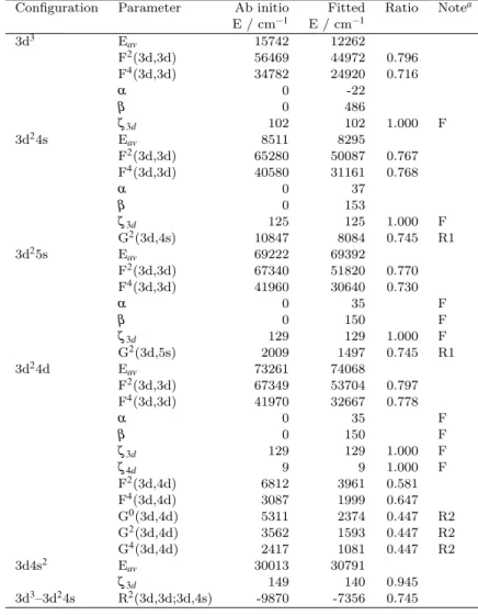
Table 5. Radial parameters adopted in the HFR+CPOL calculations for the 3d3, 3d24s, 3d25s, 3d24d and 3d4s2even-parity configurations of Ti II.
Configuration Parameter Ab initio Fitted Ratio Notea E / cm−1 E / cm−1 3d3 Eav 15742 12262 F2(3d,3d) 56469 44972 0.796 F4(3d,3d) 34782 24920 0.716 α 0 -22 β 0 486 ζ3d 102 102 1.000 F 3d24s E av 8511 8295 F2(3d,3d) 65280 50087 0.767 F4(3d,3d) 40580 31161 0.768 α 0 37 β 0 153 ζ3d 125 125 1.000 F G2(3d,4s) 10847 8084 0.745 R1 3d25s E av 69222 69392 F2(3d,3d) 67340 51820 0.770 F4(3d,3d) 41960 30640 0.730 α 0 35 F β 0 150 F ζ3d 129 129 1.000 F G2(3d,5s) 2009 1497 0.745 R1 3d24d E av 73261 74068 F2(3d,3d) 67349 53704 0.797 F4(3d,3d) 41970 32667 0.778 α 0 35 F β 0 150 F ζ3d 129 129 1.000 F ζ4d 9 9 1.000 F F2(3d,4d) 6812 3961 0.581 F4(3d,4d) 3087 1999 0.647 G0(3d,4d) 5311 2374 0.447 R2 G2(3d,4d) 3562 1593 0.447 R2 G4(3d,4d) 2417 1081 0.447 R2 3d4s2 E av 30013 30791 ζ3d 149 140 0.945 3d3–3d24s R2(3d,3d;3d,4s) -9870 -7356 0.745 a F: fixed parameter value; Rn : Fixed ratio between these parameters.
Table 6. Radial parameters adopted in the HFR+CPOL calculations for the 3d24p and 3d4s4p odd-parity configurations of Ti II. Configuration Parameter Ab initio Fitted Ratio Notea
E / cm−1 E / cm−1 3d24p E av 37888 38418 F2(3d,3d) 66208 50859 0.768 F4(3d,3d) 41202 29899 0.726 α 0 49 β 0 85 ζ3d 127 127 1.000 F ζ4p 176 176 1.000 F F2(3d,4p) 14522 11668 0.803 G1(3d,4p) 6343 5603 0.883 G3(3d,4p) 5111 3249 0.636 3d4s4p Eav 56603 59030 ζ3d 150 150 1.000 F ζ4p 236 236 1.000 F F2(3d,4p) 15975 14378 0.900 G2(3d,4s) 10055 8363 0.832 G1(3d,4p) 9785 6346 0.649 G3(3d,4p) 5244 3136 0.598 G1(4s,4p) 38957 25804 0.662 3d24p–3d4s4p R2(3d,3d;3d,4s) -6658 -4420 0.664 R R2(3d,4p;4s,4p) -13417 -8906 0.664 R R1(3d,4p;4s,4p) -13786 -9152 0.664 R a F: fixed parameter value; R: Fixed ratio between these parameters.
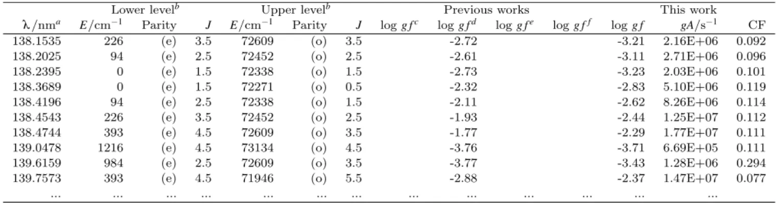
Table 7. Radiative transition rates for Ti II spectral lines. The full table is available online.
Lower levelb Upper levelb Previous works This work
λ /nma E/cm−1 Parity J E/cm−1 Parity J log g fc log g fd log g fe log g ff log g f gA/s−1 CF
138.1535 226 (e) 3.5 72609 (o) 3.5 -2.72 -3.21 2.16E+06 0.092
138.2025 94 (e) 2.5 72452 (o) 2.5 -2.61 -3.11 2.71E+06 0.096
138.2395 0 (e) 1.5 72338 (o) 1.5 -2.73 -3.23 2.03E+06 0.101
138.3689 0 (e) 1.5 72271 (o) 0.5 -2.32 -2.83 5.10E+06 0.119
138.4196 94 (e) 2.5 72338 (o) 1.5 -2.11 -2.62 8.26E+06 0.114
138.4543 226 (e) 3.5 72452 (o) 2.5 -1.93 -2.44 1.25E+07 0.112
138.4744 393 (e) 4.5 72609 (o) 3.5 -1.77 -2.29 1.77E+07 0.111
139.0478 1216 (e) 4.5 73134 (o) 4.5 -3.76 -3.71 6.69E+05 0.111
139.6159 984 (e) 2.5 72609 (o) 3.5 -3.77 -3.43 1.28E+06 0.294
139.7573 393 (e) 4.5 71946 (o) 5.5 -2.88 -2.37 1.47E+07 0.077
... ... ... ... ... ... ... ... ... ... ... ... ...
a Wavelengths (in vacuum/air below/above 200 nm) deduced from experimental energy levels.
b Experimental energy levels taken fromHuldt et al.(1982) andSaloman(2012). (e) and (o) stand for ’even’ and ’odd’, respectively. cPickering et al.(2001)
d Kurucz(2011) eWood et al.(2013)