HAL Id: hal-02871130
https://hal.archives-ouvertes.fr/hal-02871130
Preprint submitted on 17 Jun 2020HAL is a multi-disciplinary open access
archive for the deposit and dissemination of sci-entific research documents, whether they are pub-lished or not. The documents may come from teaching and research institutions in France or abroad, or from public or private research centers.
L’archive ouverte pluridisciplinaire HAL, est destinée au dépôt et à la diffusion de documents scientifiques de niveau recherche, publiés ou non, émanant des établissements d’enseignement et de recherche français ou étrangers, des laboratoires publics ou privés.
Radiofrequency heating measurement in vivo using MR
thermometry and field monitoring: methodological
considerations
Caroline Le Ster, Franck Mauconduit, Christian Mirkes, Michel Bottlaender,
Fawzi Boumezbeur, Boucif Djemai, Alexandre Vignaud, Nicolas Boulant
To cite this version:
Caroline Le Ster, Franck Mauconduit, Christian Mirkes, Michel Bottlaender, Fawzi Boumezbeur, et al.. Radiofrequency heating measurement in vivo using MR thermometry and field monitoring: methodological considerations. 2020. �hal-02871130�
1 Radiofrequency heating measurement in vivo using MR thermometry and field monitoring: methodological considerations
Caroline Le Ster1, Franck Mauconduit1, Christian Mirkes2, Michel Bottlaender3,4, Fawzi
Boumezbeur1, Boucif Djemai1, Alexandre Vignaud1, Nicolas Boulant1
1Université Paris-Saclay, CEA, CNRS, BAOBAB, NeuroSpin, 91191, Gif-sur-Yvette, France
2Skope MRT, Zurich, Switzerland
3Université Paris-Saclay, CEA, CNRS, Inserm, BioMaps, Service Hospitalier Frederic Joliot,
91401, Orsay, France
4UNIACT, Neurospin, CEA, 91191, Gif-sur-Yvette, France
Corresponding author: Nicolas Boulant, NeuroSpin, CEA, Université Paris-Saclay, F-91191, Gif-Sur-Yvette,France. E-mail address: nicolas.boulant@cea.fr
2 Abstract
Purpose: A MR thermometry (MRT) method with field monitoring is proposed to improve the measurement of small temperature variations induced in brain MRI exams.
Methods: MRT experiments were performed at 7T with concurrent field monitoring and radiofrequency heating. Images were reconstructed with nominal k-space trajectories and with first order spherical harmonics correction. Experiments were performed in vitro with deliberate field disturbances, and on an anaesthetized macaque in two different SAR regimes, i.e. at 50% and 100% of the maximal SAR level allowed in the IEC normal mode of operation.
Results: Inclusion of magnetic field fluctuations in the reconstruction improved temperature measurement accuracy in vitro down to 0.02°C. Measurement precision in vivo was on the order of 0.15°C in areas little affected by motion. In the same region, temperature increase reached 0.2°C and 0.5°C after 20 minutes of heating for the 50% and 100% SAR scans, respectively. A temperature plateau as predicted by Pennes’ bioheat model was not observed. Conclusion: Inclusion of field fluctuations in image reconstruction was beneficial for the measurement of small temperature rises encountered in standard brain exams. More work is needed to correct for motion-induced field disturbances to extract reliable temperature maps.
Key words: MR thermometry, field monitoring, radiofrequency heating, proton resonance frequency shift, ultra-high field.
3 Introduction
Several MR thermometry (MRT) methods have been developed to monitor non-invasively temperature variations during thermal therapies (1) but also for RF heating evaluations (2). The proton resonance frequency shift (PRFS) method is based on the change of the water-bound fraction with temperature that induces a local frequency shift of water spins proportional to temperature (3). In biological tissues with high water content, this shift is equal to -0.01 ppm/°C, independently of the tissue considered (4). The sensitivity of the PRFS method increases with the magnetic field and reaches -3 Hz per 1°C at 7T. PRFS is reputed as the most accurate MRT strategy available (5), especially to assess small temperature changes (6). It is nevertheless impaired by external sources of frequency shift (e.g. B0 field drift, breathing,
cardiac pulsation and limb motion for brain MRT), that can be extremely severe, especially at high magnetic field, thus counterbalancing the amplified frequency shift versus temperature with field strength. In addition, since temperature mapping is generally computed from a phase difference by subtracting a reference phase map acquired before heating, the PRFS method is also very sensitive to motion (7). Several solutions have been proposed to overcome these problems (1,8). For instance, self-referenced approaches derive the reference phase information from the same image as the one used for temperature measurement. This information can be inferred from surrounding non-heating voxels for thermal therapy MRT applications (9,10), or from fatty tissues provided lipid temperature-induced susceptibility changes are negligible (11). Other methods make use of reference phase maps and correct bias with approaches such as navigator echoes (12), FID navigators (13,14), multi-baseline reconstruction (15) and post-processing algorithms (16,17).
During an MR exam, the temperature rise in the brain induced by radiofrequency (RF) exposure must be such that absolute temperature remains below 39°C and temperature rise in the eyes must not exceed 1°C according to International Electrotechnical Commission guidelines released in 2010 (18). The gold standard for absolute temperature prediction is Pennes’ bioheat equation (19):
𝜌𝐶 = ∇𝑘. ∇𝑇 + 𝑘∇²𝑇 + 𝑄 − 𝐵(𝑇 − 𝑇 ) + 𝜌𝑆𝐴𝑅 [1]
Where ρ is the tissue density (kg/m3), C
p the specific heat capacity (J/kg/K), T the absolute
temperature (K), k the thermal conductivity (W/m/K), Q the metabolic heat generation (W/m3),
B the perfusion coefficient (W/m3/K), Tb the arterial blood temperature (K) assumed constant
at 37°C in this model, and SAR (W/kg) the specific absorption rate corresponding to RF power deposition. In this equation, the first term on the right-hand side can often be neglected because of relatively similar thermal conductivities in brain tissues. Heat diffusion being a slow process (characteristic length 𝑙 = 6𝑘𝑡 𝜌𝐶⁄ ≈ 2𝑐𝑚 for grey matter after 10 minutes), the
4 diffusion term can also be neglected for short heating times and smooth temperature profiles, whereby temperature increase is linear with SAR and time. In phantom measurements with a head coil (20), this linear approximation remained valid even for up to 10 minutes. For longer heating times, the action of diffusion superimposes to the one of perfusion and acts as a Gaussian smoothing kernel. It was furthermore shown that the actions of perfusion and diffusion could be alternated to speed up computation and still reach good accuracy (21). As a result, in a first approximation, the temperature rise in the tissues for relatively short heating times and smooth heating patterns can be analytically solved using the following equation:
𝑇(𝑡) ≈ 1 − exp (− ) [2]
Where T(t) denotes the temperature rise as opposed to absolute temperature in Eq. (1). According to Eq. (2), temperature should reach a plateau due to an equilibrium between energy deposition and blood cooling after 3, where =ρCp/B. Considering = 1000 kg/m3 in both
white and grey matter, Cp = 3600 J/kg/K in white matter (3700 J/kg/K in grey matter) and B =
16000 W/m3/K in white matter (45000 W/m3/K in grey matter) (22), quasi-equilibrium should be
reached after approximately 12 min for white matter and 4 min for grey matter. However there has been only limited in vivo data available validating this model. Direct measurements of RF induced brain heating were performed using fluoroptic probes in anaesthetized swine (23–25) along with MRT studies on an anesthetized baboon (13) and calves of human volunteers (2). In these studies, temperature was monitored continuously during RF exposure, but no plateau was captured. Yet it is not clear how the invasiveness of the optical probe measurements or anesthesia could affect temperature in the animal studies. In low-perfused tissues such as skin and muscle, observing a plateau also requires long acquisition times, with non-negligible diffusion effects, and thus reliable methods to extract quantitative MRT information.
To date, measuring temperature rise maps on the order of 1°C in vivo and non-invasively has been a great challenge, hampering efforts to validate Pennes’ bioheat model in normal conditions and on volunteers. The accuracy of the PRFS method suffers from field disturbances and because RF fields generated by MR coils induce relatively spread and smooth temperature rises, self-referenced approaches cannot be easily used (26). NMR field sensors have shown great efficiency in monitoring and correcting in vivo for spatiotemporal field fluctuations up to the third order of the spherical harmonics decomposition, encompassing magnetic field fluctuations related to scanner instabilities, head or limb motion and physiology (27). The aim of the current study was to assess the ability of field monitoring to retrospectively correct RF induced temperature rises measured with the PRFS method at 7T to increase accuracy and precision. Such methodology could be useful to explore the safety limits enforced during MRI examinations and confront SAR levels estimated in numerical simulations to
5 experimental temperature rises (28). Phantom experiments with deliberate field disturbances are first presented and are compared with optical probe measurements to validate the method. Preliminary measurements on an anaesthetized macaque are also reported as an attempt to detect the plateau of temperature predicted by the Pennes’ model.
Methods
Data acquisition Study design
MRT experiments were performed on an agar-gel phantom and on one anaesthetized macaque with a 2D-GRE sequence that was run continuously in normal SAR conditions. Magnetic field fluctuations related to scanner instabilities, head or limb motion and physiology (cardiac and breathing cycles etc...) that occurred during the scans were recorded using 16 field sensors. They were used to reconstruct retrospectively the MR images with a spherical harmonics decomposition that included field coefficients of the zeroth and first order (i.e. B0,
Gx, Gy and Gz terms) (27). For the phantom experiment, temperature was also measured with an optical probe (FISO Technologies Inc., Quebec, Canada) to establish reference values. As a first step, the accuracy and precision of this thermometry protocol was assessed by running a 20 minutes scan (10 minutes for the macaque) with a SAR inferior to 1% of the maximum level allowed by the scanner in its normal mode of operation, i.e. with maximum global and 10 g peak SAR equal to 3.2 W/kg and 10 W/kg respectively (18), according to numerical simulations performed by the coil manufacturer and incorporating a safety factor of approximately 2. No measurable temperature change was expected to occur during this scan, thereafter referred to as stability scan. As the next step, the ability of this method to detect a temperature change was tested by running scans with concurrent RF heating. Energy was deposited by means of a non-selective high-energy RF pulse that was added before the excitation pulse in the 2D-GRE sequence. This pulse was played by the transmission imaging coil and with 100 kHz offset from the water resonance to avoid spin excitation, enabling continuous imaging and temperature measurement (29). To possibly observe the temperature plateau of Eq. (2) on the macaque, the heating scan duration was set to 20 minutes.
Given that scans and RF heating ran continuously during tens of minutes, the phase of in vivo images was corrupted by motion. To account for this, the 2D-GRE sequence was acquired in 3 orthogonal planes (sagittal, coronal and transversal slices acquired in a sequential manner) for subsequent 3D motion tracking. Images were thus used for both thermometry measurements and motion estimate. A schematic view of the study is given in Figure 1.
6 MR imaging
MR scans were performed on a Magnetom 7T scanner (Siemens Healthineers, Erlangen, Germany) equipped with the Nova 1Tx-32Rx head coil (Nova Medical, Wilmington, MA, USA). A second order shim was performed prior to the imaging scans that consisted in an anatomical sequence followed by reference scans (used for B0 mapping and sensitivity profile estimation),
MRT stability and heating scans.
The anatomical sequence was an MPRAGE with TR/TE/TI 3070/2.8/1100 ms, flip angle 9°, 1 mm isotropic resolution, 160 sagittal slices, FOV 256 mm, parallel imaging with GRAPPA (R=2), resulting in an acquisition time of 6:41 min. Reference scans were performed with a single-slice 2D-GRE sequence that included 4 echoes and TR 28 ms, TE1/TE2/TE3/TE4
2.67/3.41/4.15/4.89 ms, 3x3x5 mm3 resolution, FOV 192 mm, flip angle 4°, pixel bandwidth
2000 Hz/Px. Three reference scans were acquired: one in the sagittal plane, one in the coronal plane and one in the transversal plane. The 2D-GRE MRT scans were performed in the same three planes with same bandwidth per pixel and resolution. Other parameters were: TR 28 ms, TE 22 ms in vitro and 15 ms in vivo, excitation pulse flip angle 10°, acquisition time per slice 1.8 s, rectangular heating pulse of 3.5 ms with 100 kHz offset. The heating pulse was disabled for the stability scan. For the heating scans the flip angle was adjusted to reach the desired SAR level.
Magnetic field monitoring
The field sensors setup (Skope MRT, Zurich, Switzerland), consisting of 16 19F NMR field
probes, was positioned on the receive part of the coil. This setup was used to record the magnetic field evolution concurrently with the image acquisition every 112 ms. The data of the field probes was used to perform a spatial field expansion on a full 2nd order spherical
harmonics basis (i.e. k0, kx, ky, kz and five additional terms). The skipped k-space lines that could not be monitored due to the short TR (28 ms) of the 2D-GRE scan were interpolated.
Phantom validation
This protocol was first tested on a 16-cm diameter spherical water phantom composed of 1% agar and doped with a mixture of CuSO4 (0.25 g/L) and NaCl (4 g/L). Reference temperature
was monitored with a fiber optic probe inserted in the phantom, and its position was determined using a proton-density weighted image. Three MRT experiments were performed on the
7 phantom. The first experiment was used to determine the frequency shift per degree Celsius (, in ppm/°C) in the phantom by maximizing the correlation between MRT and optical probe measurements. It consisted in a 35 minute long scan (392 series of sagittal, coronal and transversal slices) designed as follows: 5 minutes without heating but with low-SAR imaging, followed by 20 minutes at maximal SAR (100% of the level allowed by the scanner in its normal mode of operation) and then 10 minutes without heating. The second experiment was performed to test the robustness of the method to field disturbances. The same settings as in the first experiment were used while the field was disturbed between the 15th and 20th minutes
of the scan by moving a second water phantom at the entrance of the scanner tunnel. The third experiment was a 20-minute stability scan performed to quantify the accuracy and precision of the method in this ideal motionless case.
In vivo scans
The phase stability of in vivo images in the MRT context is very sensitive to motion (7), especially at high field. Motion-induced field disturbances caused by motion of sources located inside the head (air cavities) are not well captured by the field sensors which assume external and smooth fluctuations decomposable into low-order spherical harmonics (27). In order to limit the impact of motion on temperature measurements, in vivo experiments were performed on an anaesthetized macaque (Macaca mulatta adult male, weight 10 kg) placed in the supine position. This study was conducted in accordance with the European convention for animal care and the NIH’s Guide for the Care and Use of Laboratory Animals, and was approved by the institutional ethical committee (CETEA protocol A19-012). For anesthesia induction, the animal received an intramuscular injection of ketamine and medetomidine (0.4/0.4 mL) and the anesthesia was maintained using sevoflurane (1%) with 50/50 air/O2 mix. The macaque
was covered with a non-heating blanket, intubated and mechanically ventilated with a respiration rate of 18 cycles/min. Physiological monitoring included heart rate, oxygen saturation, respiratory rate, expired/inspired sevoflurane concentration and end-tidal CO2.
Antisedan (0.2 mL) was used to wake up the macaque after the MR examination. MRT scans acquired on the macaque had a TE of 15 ms to counteract rapid signal decay due to large nasal cavities. Heating scans of 100% and 50% maximum SAR were carried out, followed by a stability scan. MRT scans were separated by 10 min breaks to allow returning to basal conditions. The stability scan was 10 min long, while the heating scans were 35 min long (same design as the phantom heating scans, i.e. 5 min pre-RF heating, 20 min RF heating and 10 min post-RF heating). Given the supposedly small temperature rises induced in these MRI normal conditions, no significant changes in Eq. (1) thermal parameters were expected (30).
8 Post-processing
Image reconstruction
Image reconstruction was carried out offline using the skope-i software (Skope MRT, Zurich, Switzerland). In a first step, B0 maps and coil sensitivity profiles were estimated from the
sagittal, coronal and transversal reference scans. In a second step, these B0 maps were used
to reconstruct images of the individual channels of the MRT scans using either 1) the nominal Cartesian k-space trajectories (referred to as nominal images), or 2) the actual trajectories recorded by the field sensors with additional B0 fluctuation correction (corrected images)
through an iterative conjugate gradient algorithm that included zeroth and first order field coefficients of the spherical harmonics (i.e. k0, kx, ky and kz terms) (31). Spherical harmonics correction was limited to the first order terms due to greater uncertainty on the coefficients of the second order. Complex combined images were reconstructed by multiplying the individual coil images by their respective sensitivity profiles and summing them.
Sensitivity to motion
Despite anesthesia, in vivo MRT images were still affected by motion, inferred as a fast (slice-to-slice) motion caused by cardiac pulsation and a slow motion due to muscle relaxation. As a preliminary step, influence of motion on the phase was estimated with numerical simulations. The method of Salomir et al. (32) was applied on the human head model described in (33,34) while the field direction was rotated to mimic motion while avoiding discretization errors (35). Field maps of the brain shimmed to the second order were simulated with an isotropic resolution of 1 mm, then the field was rotated by 2° around either the Left-Right (LR), Anteroposterior (AP) or Head-Foot (HF) axis to simulate a head rotation. The effect of a 1 mm translation in each direction was also tested. A numerical model of the macaque not being available, the main purpose of these simulations was to provide rough guidelines and intuition about the sensitivity of the phase versus motion.
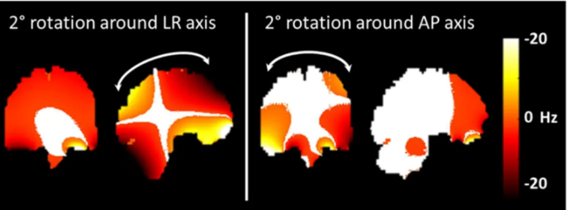
The simulations (Figure 2) showed that rotations around the LR axis impacted particularly the resonance frequency on the frontal lobe and on the cerebellum, while rotations around the AP axis impacted the temporal lobes. Furthermore, the LR rotation left only a small region of the brain with less than 1 Hz shift. Rotations around the HF axis and translations barely affected the resonance frequency. The center of the brain appeared the area of the brain the most robust to motion. Thus, the 2D-GRE acquisition scheme was decided based upon these observations. A small area in the sagittal view may be reasonably robust to rotations around
9 AP and HF axis, while a higher sensitivity to a rotation around LR axis may require additional means to correct for it, provided the rotations are known. As a result, three orthogonal slices were sequentially acquired to capture rotation parameters while the main temperature measurement focus was in the sagittal view.
Figure 1: Frequency shift induced by head rotations. Frequency shift induced by head rotations of 2° around the Left-Right (LR) and Anteroposterior (AP) axis on the coronal and sagittal planes. Areas with a frequency shift inferior to 1 Hz appear in white.
Motion-based phase and temperature correction
Motion parameters were estimated on magnitude images with McFlirt (36) as follows: for each orthogonal plane, the 55 first images of the time series, corresponding to the first five minutes of the scan without RF heating, were averaged to create a new template image (15). This template image was then used as a reference to register the whole time series with 3 degrees of freedom (1 rotation and 2 translations), so that a total of 3 rotation and 6 translation parameters were estimated for each scan. Only rotations were taken into account in the processing pipeline given their superior impact found in the simulations but also to minimize the amount of post-processing. Motion parameters were estimated separately for nominal and field-sensors corrected images.
The rotation parameters estimated on magnitude images were then used to correct phase images. For each MRT scan, images acquired during the first five minutes were used as a dictionary to estimate the influence of rotation parameters on the phase of each voxel (37). Indeed, as no heating pulse was applied during this period, phase variations were considered to be caused only by head rotations. To estimate the influence of the rotation parameters on the phase on each voxel, a linear regression corrected for the voxel mean signal was performed. The resulting coefficients were then applied to the whole time series as an attempt
10 to compensate for head rotations in the heating and post-heating periods. Likewise, this correction was applied to both nominal and field-sensors corrected images.
Temperature computation
Temperature change at time t and position r was computed from nominal and corrected images as:
∆𝑇 (𝑟⃗) = ∆ ( ⃗) [3]
where ΔTt is the temperature change (°C), Δϕt is the phase difference between time t and a
reference (rad), is the Larmor frequency (Hz), α is the frequency shift per degree Celsius (-0.01 ppm/°C in vivo (4)) and TE is the echo time (s).
Results
Phantom results
The value of α for the phantom was determined using images of the first heating scan that were corrected for first order spherical harmonics field fluctuations. Fitting the phase measured at probe location to probe recordings yielded α = -0.015 ppm/°C (R2 = 0.99). Resulting
temperature variation maps (Figure 3a), computed after 20 minutes of RF heating, showed a hotspot located at the back of the coil, where temperature rise reached 0.6°C and 0.7°C for the nominal and corrected images, respectively. The latter resulted in higher temperature rise due to field drift correction in the reconstruction pipeline. Interestingly, Figure 3a shows that the nominal and corrected scenarios do not merely differ by a global temperature offset (mean difference 0.11°C, standard deviation of the difference 0.04°C) that could simply be corrected by zeroth-order B0 correction.
Results at probe location for the heating scan performed with field disturbances (Figure 3b) show that the major field changes induced by a secondary phantom movement in the scanner tunnel were captured by the field probes and corrected to a large extent, whereas the uncorrected approach naturally failed.
11 Figure 2: Heat scan results for the phantom. (a) Sagittal, coronal and transversal maps of the temperature variation computed after 20 minute scan at the maximal SAR level allowed by the scanner manufacturer in the normal mode of operation. These maps were computed from images reconstructed with nominal trajectories (upper row) and trajectories corrected with first order spherical harmonics fluctuations (lower row). (b) Temperature variation measured by the fiber optical probe and from nominal and field sensors-based corrected MRT images at probe location, in field disturbed conditions.
During the stability scan, the fiber optic probe recorded a slow temperature rise (+0.03°C over 20 minutes, Figure 4) that the field-sensor correction scheme was able to capture. The root mean square error computed between fiber optical probe data and MRT measurements was 0.034°C for the nominal images and 0.021°C for the corrected images. Inclusion of spherical harmonics correction in the reconstruction corrected for the drift, but not for the noise peak-to-peak amplitude, which was comparable for both reconstruction methods in this in vitro scenario.
12 Figure 3: Stability scan results for the phantom. Temperature variation measured by the fiber optical probe and from nominal and field sensors-based corrected MRT images at probe location over the 20 minutes scan at <1% of the maximal SAR.
Macaque scans
Nominal and corrected temperature maps computed for the macaque brain during the stability scan are overlaid over their anatomical reference image in Figure 5a. The average temperature variation computed from nominal images over the time-series showed a good homogeneity over the brain and an average ΔT close to 0°C. Maps obtained from corrected images showed a gradient of temperature in the head-foot direction and an average ΔT slightly inferior to 0°C. Figure 5b displays the standard deviation map of the stability scan, calculated over the time series, the temperature being corrected for linear signal drift. As expected from the simulations, standard deviation was not homogeneous over the whole brain and reflected the sensitivity of the phase versus motion (see Figure 2). The standard deviation of the detrended signal was lower when including rotation regressors in the post-processing pipeline. No improvement here was observed when going from temperature measured from nominal images to field-sensor corrected images.
From the standard deviation maps, a voxel with low standard deviation, likely more robust to motion, was selected and its temporal signal was plotted on Figures 5e and 5f. There was a slow drift of the temperature computed from field-sensor corrected images that could not be observed on temperature computed from nominal images, as it was partly compensated by a slow B0 and kz drift. A temperature fluctuation of about 0.15°C can be observed on these plots.
There was no significant rotation of the macaque head during the stability scan (Figures 5c and d). Therefore, inclusion of rotation regressors did not affect average temperature measurement on this scan, while it reduced slightly its standard deviation.
13 Figure 4: Stability scan results for the macaque. (a) Mean and standard deviation temperature variation maps computed over a 10 minute scan without RF heating. Standard deviation maps were computed from voxel-wise detrended signals. Temperature variation maps were computed from images reconstructed with nominal trajectories (upper row) and first order spherical harmonics field correction (lower row). Temperature computed from phase images corrected with rotation regressors around LR, AP and HF axis are also displayed. (b) and (c) Rotation parameters (top) and time evolution of the temperature computed from the nominal images and corrected images, respectively, in the voxel indicated by the white cross (in a).
After 20 minutes of heating at 50% of the maximal SAR (Figure 6), temperature rise reached about 0.4°C for the nominal images (without and with rotation regressors) in the voxel of interest, -0.3°C for the field-sensor corrected images without rotation regressors and 0.2°C with rotation regressors. Field-sensor corrected images suffered from rotations around the AP axis, which resulted in negative temperatures when rotation regressors were not taken into account. During the first five minutes of the scan, when there was no heating, temperature remained constant. Then, during the heating period, temperature increased but a plateau could not be easily observed. When heating stopped, temperature kept increasing for the nominal
14 images which were affected by field drift, while it decreased for field-sensor corrected images, as expected. Fitting Eq. (2) to the heating period returned the solid lines in Figures 6b and 6c with the following time-constants: 37 (𝜒 𝑑𝑜𝑓⁄ = 1.4) and 16 (𝜒 ⁄𝑑𝑜𝑓= 0.8) min without and with regressors correction for the nominal images, respectively, versus 3 (𝜒 𝑑𝑜𝑓⁄ = 1.2) min for the field-sensor corrected images with regressors (the one without regressors returning negative temperatures). The heating scan performed at maximal SAR (Figure 7) resulted in higher temperature rise. In the voxel of interest, temperature increase reached about 0.7°C for the nominal images and 0.5°C for the corrected images, roughly yielding the expected factor of 2 compared to the scan performed at 50% of the maximal SAR. Temperature did not reach a plateau for this scan, and after the heating period the temperature decreased very slowly. In this case, the time constants for the heating periods were: 10 min for nominal images (without and with rotation regressors) (𝜒 𝑑𝑜𝑓⁄ = 1.2 and 𝜒 ⁄𝑑𝑜𝑓= 1.4) versus 10 (𝜒 ⁄𝑑𝑜𝑓= 1.1) and 12 (𝜒 𝑑𝑜𝑓⁄ = 1.1) min for field-sensor corrected images without and with rotation regressors, respectively.
Figure 5: 50% Heat scan results for the macaque. (a) Temperature variation maps computed after 20 minute scan at 50 % of the maximal SAR. These maps were computed from nominal images (upper row) and corrected images (lower row), without (left column) and with (right column) inclusion of rotation regressors around LR, AP and HF axis in the post-processing pipeline. (b) and (c) Time evolution of temperature variation computed from the nominal images and corrected images, respectively, in the voxel indicated by the white cross in (a). Temperature rise during the RF-heating period was fitted to Pennes’ simplified equation (Equation 2) to yield the solid lines.
15 Figure 6: 100% Heat scan results for the macaque. (a) Temperature variation maps computed after 20 minute scan at maximal SAR. These maps were computed from nominal images (upper row) and corrected images (lower row), without (left column) and with (right column) inclusion of rotation regressors around LR, AP and HF axis in the post-processing pipeline. (b) and (c) Time evolution of temperature variation computed from the nominal images and corrected images, respectively, in the voxel indicated by the white cross in (a). Solid lines represent the fit of Equation (2) during the RF heating periods.
Discussion and conclusion
In this study, correction of magnetic field fluctuations measured with field sensors up to the first order of the spherical harmonics decomposition improved the accuracy of temperature measurement in a phantom, especially when the field was disturbed. It also showed that beyond zeroth-order correction as it is commonly done with fat-referenced techniques had a non-negligible impact. Provided field disturbances are smooth enough, they can be well captured by a relatively small number of NMR field probes. When applying such methodology in vivo, even if nominal images could yield comparable results to the corrected ones, the field disturbance experiment data in general boosts confidence in the results obtained with field monitoring and in vivo. In the brain of the anaesthetized macaque, such a correction allowed retrieving the slow temperature decay, possibly provoked by anesthesia (38). While inclusion of magnetic field fluctuations in the reconstruction improved the accuracy of the measurement, it did not improve its precision which yielded about 0.15°C in the macaque brain.
Field corrections to the first order of the spherical harmonics decomposition were shown sufficient to remove most artefacts in T2*-weighted acquisitions (39), so that inclusion in the
current study of higher order terms would not likely improve data quality significantly. Most of the noise in the time series appeared to originate from the cardiac pulsation and resulted in a periodical motion of the brain. Methods aiming at reducing noise in PRFS temperature
16 measurements (15–17) were not implemented here in order to minimize the amount of post-processing for a fair comparison between image reconstruction methods. Despite anesthesia, the influence of motion on the phase turned out to be high in some regions (7). As a result, reliable estimate of small temperature rises everywhere in the brain was rendered difficult. Based on simulation, the strategy used here was to focus on a sagittal slice to possibly observe a temperature hotspot as measured in phantom studies with the same coil (20) and attempt detecting a temperature plateau in a zone relatively robust to head motion. In addition to focusing on a brain zone little affected by motion, the inclusion of head motion regressors in the post-processing pipeline appeared helpful. This correction however suffered from several weaknesses, so that the phase of voxels located in the outer parts of the brain was too corrupted to be corrected. Images were indeed acquired with both low spatial and temporal resolutions, especially since they were acquired in the sagittal, coronal and transversal planes sequentially to estimate motion in every orientation, which could explain discrepancies between nominal and corrected images. A better estimate of motion and faster acquisition schemes could potentially improve temperature measurement. External devices were recently developed to monitor head motion at no time cost (e.g. optical tracking), but no such device was available on site. Another way of improving motion detection would be to accelerate image acquisition, both to reduce intrascan motion and to increase the sampling frequency. Parallel imaging was not used in the current study because sensitivity profiles could only be estimated from a scan acquired at the beginning of the time series in the image reconstruction software, which is not accurate when motion occurs. Faster image acquisition could also be achieved, for instance through acquisition schemes such as the EPI sequence (40), so that motion parameters could be more reliably estimated with 3D brain volumes.
After 20-minute heating at the maximal SAR level allowed by the scanner in its normal mode of operation, an increase of approximately 0.5°C was measured in the center of the macaque brain. The rise was about twice lower when the SAR was halved. The power deposited by the heating pulse was 5.5 W for the scan at 50% of the maximal SAR and 11 W for the scan at maximal SAR. According to (20), where a pulse of 16 W resulted in a local SAR hotspot of 6 W/kg in a head phantom, in the current study the corresponding local SAR hotspot could reach 2 W/kg and 4 W/kg for the 50% and 100% SAR scans, respectively. The heating scan performed at 50% SAR, reconstructed with field sensor-recorded trajectories and corrected for motion, returned a reasonable time constant of 3 minutes for the fit of Eq. (2) but was not reproduced at higher SAR. The standard deviation of this scan was however relatively high relative to its mean signal. At maximal SAR, no plateau was reached during the 20-minute heating period and the data seemingly more robust to motion returned a time constant of up to 12 minutes, far from what is expected from the literature for white and gray matter (22). The
17 use of anesthetic agents could explain the deviation from the expected behavior. A thermoregulation study performed on macaques showed that ketamine did not disturb the vasomotor response of the animals but that it slightly reduced sweating and tended to increase body temperature in high temperature regimes (38). A slow increase of blood temperature could thus have occurred during heating experiments and may have prevented from reaching the expected plateau. This could however not be verified since the macaque body temperature was not monitored during the experiment. The size of the macaque was relatively small compared to the coil, so that approximately a third of the macaque volume fitted into it and was thus exposed to the heating pulse, possibly leading to an increase in the macaque body temperature. In addition, heat diffusion may have occurred during the cooling period and could explain the slow temperature decay in the last period that did not return to its initial value after 15 minutes. In the literature, studies that recorded the temperature continuously during RF-heating experiments also failed to observe such a plateau (2,13,23–25). These studies were however all performed on anaesthetized animals or on lowly perfused organs which may have prevented the expected plateau to arise. More complex models, that include additional parameters, were proposed to better estimate tissue temperature (41,42). It certainly calls for additional work to investigate such effects on human volunteers and in normal MRI conditions. A thorough validation of Pennes’ model remains highly desirable to strengthen confidence in the numerical safety assessments in MRI exams (28) as well as to possibly boost performance at ultra-high-field (43,44).
Limits of this study include the absence of reference temperature recordings in vivo and the fact that measurements were performed only on one macaque. They should be thus considered preliminary. The results obtained in vitro nevertheless demonstrate that the use of field sensors increased the confidence in the temperature measurements, which can supposedly be transposed in vivo. Further developments are required to better handle motion and apply this method on humans. Yet, it should be stressed that even prospective motion correction techniques (45) would not solve the problem because they address the geometrical consistency of the data acquisition and not the motion-induced field changes. Head fixation (https://caseforge.co/) and post-processing methods based on dictionaries or simulations appear possible candidates.
In conclusion, this study showed the benefits of including correction of the magnetic field perturbations up to the first order of the spherical harmonics decomposition in PRFS temperature measurements. Phantom measurements with deliberate field disturbances as well as preliminary measurements on an anaesthetized macaque were presented. Head motion-induced field changes appear a daunting challenge to measure accurately temperature maps non-invasively in vivo and in normal MRI RF exposure conditions. Given these great obstacles,
18 an intermediate goal is proposed to be the qualitative validation of Pennes’ model with the observation of a temperature plateau in highly perfused tissues and in conditions (time-scales, heating patterns) where heat diffusion can be safely neglected.
Acknowledgements
We thank D. Brunner, C. Barmet, K. Pruessmann, L. Winter for valuable discussions and P. Ehses for providing the Skope-enabled GRE sequence. This work received financial support from Leducq Foundation (large equipment ERPT program, NEUROVASC7T project), and from the European Union Horizon 2020 Research and Innovation program under Grant Agreement No. 736937 (M-Cube project) (except for the animal experiments). Michel Bottlaender, Fawzi Boumezbeur and Boucif Djemai performed the in vivo experiments on the macaque. The other authors planned the experiments, did the phantom measurements and analyzed the data.
References
1. Rieke V, Pauly KB. MR thermometry. J. Magn. Reson. Imaging 2008;27:376–390 doi: 10.1002/jmri.21265.
2. Simonis FFJ, Raaijmakers AJE, Lagendijk JJW, van den Berg CAT. Validating subject-specific RF and thermal simulations in the calf muscle using MR-based temperature measurements: Validating RF and Thermal Simulations with MRI Measurements. Magn. Reson. Med. 2017;77:1691–1700 doi: 10.1002/mrm.26244.
3. Hindman JC. Proton Resonance Shift of Water in the Gas and Liquid States. J. Chem. Phys. 1966;44:4582–4592 doi: 10.1063/1.1726676.
4. Peters RTD, Hinks RS, Henkelman RM. Ex vivo tissue-type independence in proton-resonance frequency shift MR thermometry. Magn. Reson. Med. 1998;40:454–459 doi: 10.1002/mrm.1910400316.
5. Quesson B, Zwart JA de, Moonen CTW. Magnetic resonance temperature imaging for guidance of thermotherapy. J. Magn. Reson. Imaging 2000;12:525–533 doi: 10.1002/1522-2586.
6. Wlodarczyk W, Hentschel M, Wust P, et al. Comparison of four magnetic resonance methods for mapping small temperature changes. Phys. Med. Biol. 1999;44:607–624 doi: 10.1088/0031-9155/44/2/022.
19 7. Liu J, de Zwart JA, van Gelderen P, Murphy-Boesch J, Duyn JH. Effect of head motion on MRI B0 field distribution: Liu et al. Magn. Reson. Med. 2018;80:2538–2548 doi:
10.1002/mrm.27339.
8. Odéen H, Parker DL. Magnetic resonance thermometry and its biological applications – Physical principles and practical considerations. Prog. Nucl. Magn. Reson. Spectrosc. 2019;110:34–61 doi: 10.1016/j.pnmrs.2019.01.003.
9. Rieke V, Vigen KK, Sommer G, Daniel BL, Pauly JM, Butts K. Referenceless PRF shift thermometry. Magn. Reson. Med. 2004;51:1223–1231 doi: 10.1002/mrm.20090.
10. Salomir R, Viallon M, Kickhefel A, et al. Reference-Free PRFS MR-Thermometry Using Near-Harmonic 2-D Reconstruction of the Background Phase. IEEE Trans. Med. Imaging 2012;31:287–301 doi: 10.1109/TMI.2011.2168421.
11. Streicher MN, Schäfer A, Ivanov D, et al. Fast accurate MR thermometry using phase referenced asymmetric spin-echo EPI at high field: Fast Referenced MR Thermometry. Magn. Reson. Med. 2014;71:524–533 doi: 10.1002/mrm.24681.
12. Zwart JA de, Vimeux FC, Palussière J, et al. On-line correction and visualization of motion during MRI-controlled hyperthermia. Magn. Reson. Med. 2001;45:128–137 doi: 10.1002/1522-2594.
13. Boulant N, Bottlaender M, Uhrig L, et al. FID navigator-based MR thermometry method to monitor small temperature changes in the brain of ventilated animals. NMR Biomed. 2014 doi: 10.1002/nbm.3232.
14. Ferrer CJ, Bartels LW, Velden TA van der, et al. Field drift correction of proton resonance frequency shift temperature mapping with multichannel fast alternating nonselective free induction decay readouts. Magn. Reson. Med. 2020;83:962–973 doi: 10.1002/mrm.27985. 15. Rieke V, Instrella R, Rosenberg J, et al. Comparison of temperature processing methods for monitoring focused ultrasound ablation in the brain. J. Magn. Reson. Imaging
2013;38:1462–1471 doi: 10.1002/jmri.24117.
16. Majeed W, Schneider R, Patil S, et al. A Principal Component Analysis based Multi-baseline Phase Correction Method for PRF Thermometry. Proc. 27th Annu. Meet. ISMRM Montr. 2019:abstract 3818.
20 17. Roujol S, Denis de Senneville B, Hey S, Moonen C, Ries M. Robust Adaptive Extended Kalman Filtering for Real Time MR-Thermometry Guided HIFU Interventions. IEEE Trans. Med. Imaging 2012;31:533–542 doi: 10.1109/TMI.2011.2171772.
18. IEC. International Electrotechnical Commission. International standard, Medical equipment: particular requirements for the safety of magnetic resonance equipment, 3rd edition. Geneva. 2010.
19. Pennes HH. Analysis of Tissue and Arterial Blood Temperatures in the Resting Human Forearm. J. Appl. Physiol. 1948;1:93–122 doi: 10.1152/jappl.1948.1.2.93.
20. Insua IG, Gumbrecht R, Wicklow K, Polimeni JR. Determination of local SAR through MR Thermometry at 7T. Proc. 27th Annu. Meet. ISMRM Montr. 2019:abstract 4182.
21. Carluccio G, Erricolo D, Oh S, Collins CM. An Approach to Rapid Calculation of Temperature Change in Tissue Using Spatial Filters to Approximate Effects of Thermal Conduction. IEEE Trans. Biomed. Eng. 2013;60:1735–1741 doi:
10.1109/TBME.2013.2241764.
22. Collins CM, Liu W, Wang J, et al. Temperature and SAR calculations for a human head within volume and surface coils at 64 and 300 MHz. J. Magn. Reson. Imaging 2004;19:650– 656 doi: 10.1002/jmri.20041.
23. Eryaman Y, Lagore RL, Ertürk MA, et al. Radiofrequency heating studies on anesthetized swine using fractionated dipole antennas at 10.5 T. Magn. Reson. Med. 2018;79:479–488 doi: 10.1002/mrm.26688.
24. Nadobny J, Klopfleisch R, Brinker G, Stoltenburg-Didinger G. Experimental investigation and histopathological identification of acute thermal damage in skeletal porcine muscle in relation to whole-body SAR, maximum temperature, and CEM43 °C due to RF irradiation in an MR body coil of birdcage type at 123 MHz. Int. J. Hyperthermia 2015;31:409–420 doi: 10.3109/02656736.2015.1007537.
25. Shrivastava D, Hanson T, Kulesa J, Tian J, Adriany G, Vaughan JT. Radiofrequency heating in porcine models with a “large” 32 cm internal diameter, 7 T (296 MHz) head coil. Magn. Reson. Med. 2011;66:255–263 doi: 10.1002/mrm.22790.
26. Grissom WA, Lustig M, Holbrook AB, Rieke V, Pauly JM, Butts‐Pauly K. Reweighted ℓ1 referenceless PRF shift thermometry. Magn. Reson. Med. 2010;64:1068–1077 doi:
21 27. Barmet C, Zanche ND, Pruessmann KP. Spatiotemporal magnetic field monitoring for MR. Magn. Reson. Med. 2008;60:187–197 doi: 10.1002/mrm.21603.
28. Murbach M, Neufeld E, Cabot E, et al. Virtual population-based assessment of the impact of 3 Tesla radiofrequency shimming and thermoregulation on safety and B1+ uniformity. Magn. Reson. Med. 2016;76:986–997 doi: 10.1002/mrm.25986.
29. Ehses P, Fidler F, Nordbeck P, et al. MRI thermometry: Fast mapping of RF-induced heating along conductive wires. Magn. Reson. Med. 2008;60:457–461 doi:
10.1002/mrm.21417.
30. Bernardi P, Cavagnaro M, Pisa S, Piuzzi E. Specific absorption rate and temperature elevation in a subject exposed in the far-field of radio-frequency sources operating in the 10-900-MHz range. IEEE Trans. Biomed. Eng. 2003;50:295–304 doi:
10.1109/TBME.2003.808809.
31. Wilm BJ, Barmet C, Pavan M, Pruessmann KP. Higher order reconstruction for MRI in the presence of spatiotemporal field perturbations. Magn. Reson. Med. 2011;65:1690–1701 doi: 10.1002/mrm.22767.
32. Salomir R, de Senneville BD, Moonen CT. A fast calculation method for magnetic field inhomogeneity due to an arbitrary distribution of bulk susceptibility. Concepts Magn. Reson. 2003;19B:26–34 doi: 10.1002/cmr.b.10083.
33. Makris N, Angelone L, Tulloch S, et al. MRI-based anatomical model of the human head for specific absorption rate mapping. Med. Biol. Eng. Comput. 2008;46:1239–1251 doi: 10.1007/s11517-008-0414-z.
34. Massire A, Cloos MA, Luong M, et al. Thermal simulations in the human head for high field MRI using parallel transmission. J. Magn. Reson. Imaging 2012;35:1312–1321 doi: 10.1002/jmri.23542.
35. Marques JP, Bowtell R. Application of a Fourier-based method for rapid calculation of field inhomogeneity due to spatial variation of magnetic susceptibility. Concepts Magn. Reson. Part B Magn. Reson. Eng. 2005;25B:65–78 doi: 10.1002/cmr.b.20034.
36. Jenkinson M, Bannister P, Brady M, Smith S. Improved Optimization for the Robust and Accurate Linear Registration and Motion Correction of Brain Images. NeuroImage
22 37. Hutton C, Andersson J, Deichmann R, Weiskopf N. Phase informed model for motion and susceptibility: Phase Informed Model for Motion and Susceptibility. Hum. Brain Mapp. 2013;34:3086–3100 doi: 10.1002/hbm.22126.
38. Hunter WS, Holmes KR, Elizondo RS. Thermal balance in ketamine-anesthetized rhesus monkey Macaca mulatta. Am. J. Physiol.-Regul. Integr. Comp. Physiol. 1981;241:R301– R306 doi: 10.1152/ajpregu.1981.241.5.R301.
39. Vannesjo SJ, Wilm BJ, Duerst Y, et al. Retrospective correction of physiological field fluctuations in high-field brain MRI using concurrent field monitoring: Physiological Field Correction Using Concurrent Field Monitoring. Magn. Reson. Med. 2015;73:1833–1843 doi: 10.1002/mrm.25303.
40. Kickhefel A, Roland J, Weiss C, Schick F. Accuracy of real-time MR temperature mapping in the brain: A comparison of fast sequences. Phys. Med. 2010;26:192–201 doi: 10.1016/j.ejmp.2009.11.006.
41. Arkin H, Xu LX, Holmes KR. Recent developments in modeling heat transfer in blood perfused tissues. IEEE Trans. Biomed. Eng. 1994;41:97–107 doi: 10.1109/10.284920. 42. Shrivastava D, Vaughan JT. A Generic Bioheat Transfer Thermal Model for a Perfused Tissue. J. Biomech. Eng. 2009;131:074506 doi: 10.1115/1.3127260.
43. Boulant N, Wu X, Adriany G, Schmitter S, Uğurbil K, Moortele P-FV de. Direct control of the temperature rise in parallel transmission by means of temperature virtual observation points: Simulations at 10.5 tesla. Magn. Reson. Med. 2016;75:249–256 doi:
10.1002/mrm.25637.
44. Deniz CM, Carluccio G, Collins C. Parallel transmission RF pulse design with strict temperature constraints. NMR Biomed. 2017;30:e3694 doi: 10.1002/nbm.3694. 45. Maclaren J, Herbst M, Speck O, Zaitsev M. Prospective motion correction in brain imaging: A review. Magn. Reson. Med. 2013;69:621–636 doi: 10.1002/mrm.24314.