Walking pattern generators of biped robots using a linear pendulum model with compensated ZMP

(1)

HAL Id: hal-02116967

https://hal.archives-ouvertes.fr/hal-02116967

Submitted on 1 May 2019

HAL is a multi-disciplinary open access archive for the deposit and dissemination of sci-entific research documents, whether they are pub-lished or not. The documents may come from teaching and research institutions in France or abroad, or from public or private research centers.

L’archive ouverte pluridisciplinaire HAL, est destinée au dépôt et à la diffusion de documents scientifiques de niveau recherche, publiés ou non, émanant des établissements d’enseignement et de recherche français ou étrangers, des laboratoires publics ou privés.

Hayder Al-Shuka, Burkhard Corves, Bram Vanderborght, Wen-Hong Zhu

To cite this version:

Hayder Al-Shuka, Burkhard Corves, Bram Vanderborght, Wen-Hong Zhu. Walking pattern generators of biped robots using a linear pendulum model with compensated ZMP. [Research Report] RWTH Aachen. 2019. �hal-02116967�

(2)

Walking pattern generators of biped robots using a

linear pendulum model with compensated ZMP

Hayder F. N. Al-Shuka1, Burkhard Corves2, Bram Vanderborght3, Wen-Hong Zhu4 1 Mechanical Engineering Department, Baghdad University, Baghdad, Iraq

2 Department of Mechanism Theory, Machines Dynamics and Robotics, RWTH Aachen University, Germany 3 Department of Mechanical Engineering, Vrije Universiteit Brussel, Belgium

(3)

Abstract

This report addresses three issues of motion planning for zero-moment point (ZMP)-based biped robots. First, three methods have been compared for smooth transition of biped locomotion from the single support phase (SSP) to the double support phase (DSP) and vice versa. All these methods depend on linear pendulum mode (LPM) to predict the trajectory of the center of gravity (COG) of the biped. It has been found that the three methods could give the same motion of the COG for the biped. The second issue is investigation of the foot trajectory with different walking patterns especially during the DSP. The characteristics of foot rotation can improve the stability performance with uniform configurations. Last, a simple algorithm has been proposed to compensate for ZMP deviations due to approximate model of the LPM. The results show that keeping the stance foot flat at beginning of the DSP is necessary for balancing the biped robot.

(4)

Humans have perfect mobility with amazing control systems; they are extremely versatile with smooth locomotion. However, comprehensive understanding of the human locomotion is entirely still not analyzed.Please see [Hay19, Hay18/1, Hay18/2, Hay18/3,Hay18/4, Hay17/1, Hay17/2, Hay16, Hay15, Hay14, Hay14/1, Hay14/2, Hay14/3, Hay14/4, Hay13/1, Hay13/2, Hay13/3, Sam08] for more details on dynamics, walking pattern generators and control of biped locomotion (biped robots, lower-extremity exoskeletons, prosthetics, etc.).

Since biped robots are desired to behave as humans do, they should have a certain level of intelligence [Vuk72]. In addition, a high level of adaptability should be provided to cope with external environments. As well as, in certain circumstances, optimal motion is selected to reduce energy consumption during walking [Vuk72]. There are numerous approaches to generate the biped robot motion as detailed in Chapter 2 of [Hay14]. Most researchers concentrate on control and walking patterns of the biped robot during the SSP due to its instability and the short time of the DSP (it is about 20% during one stride of the gait cycle). However, incorporating the DSP into gait cycle is necessary to generate smooth motion of COG/hip trajectory (the hip position could be considered as an approximation of the COG position), and to stop and change walking speed as desired [Shi06, Kud03, Zhu03]. On the other hand, analysis of the DSP could result in challenging problems concerning stable walking patterns and control; the biped robot behaves as over-actuated system with constrained motion as noted in Chapters 4 and 5 of [Hay14]. To enforce the target biped to move, the analyst should generate stable trajectories for the hip and feet; the angular joint displacements and their first and second derivatives can be obtained using inverse kinematics. Therefore, the first part of this report focuses on planning methods used for generation of hip trajectory especially during the DSP. Three methods are investigated and compared to understand differences, if exist, between these methods. Then, two walking patterns 1 and 2, described in Section 2.1, with four different cases are considered to understand the behavior of feet motion and the effect of impact on the biped configuration. Consequently, four different feet trajectories are encountered. Piecewise spline functions are used to approximate the feet trajectories during the SSP; whereas, foot rotation during the DSP is exactly arc. Above all, stability of biped locomotion is needed to be evaluated because these analyses depend on approximate model represented by inverted pendulum which can result in deviations of ZMP trajectories. Therefore, the last part introduces solutions to the above. First, it proposes a thorough algorithm to tune walking parameters (hip height, distance traveled by the hip, and the times of the SSP and the DSP) and to satisfy specified kinematic and dynamic constraints. Second, it derives exact trigonometric relationships for feet trajectories during the DSP rather than the piecewise spline functions used in some works such as [Hua99, Hua01]. This can avoid deviations in the velocity and acceleration of the feet

(6)

at the transition instances of the walking cycle resulting in continuous dynamic response for the biped mechanism.

The structure of this report is as follows. Section 1.1 evaluates comparative studies of

generation of walking patterns during the complete gait cycle, especially for the DSP.

Whereas, Section 1.2 introduces a simple algorithm for generating stable biped walking

compensating ZMP deviations. Section 1.3 presents simulation results and discussions.

Section 2 concludes.

1.1 A comparative study for generation of biped walking patterns

1.1.1 COG (hip) trajectory

It is verified that designing a suitable COG trajectory can ensure stable dynamic motion for biped robots [Hua99, Hua01]. We can classify two essential methods regarding this topic. The first one includes designing polynomial functions (or piecewise spline functions) for the COG trajectory during the complete gait cycle satisfying the constraint and continuity conditions [Hua99, Mu03, Tan03]. This method selects the COG trajectory with largest stability margin represented by the zero-moment point (ZMP) stability margin. In contrast, the second method suggests employing a simple dynamic model for the biped robot denoted by the linear inverted pendulum mode (LIPM) [Kaj96, Kud03, Shi06]. Consequently, the notion of pendulum mode has been exploited for generation of stable COG motion. Designing walking pattern for biped mechanism without the DSP can lead to discontinuity of COG acceleration

at switch (transition) instances as seen in Fig. 1-1 and Fig. 1-2; the DSP can mainly improve

dynamic response at the expense of further computation. Below we will discuss three important methods used in literature for describing the motion of the COG trajectory during the two gait phases guaranteeing continuous transition between the phases. The following three methods have been used as walking generators for biped locomotion during complete gait cycle:

1.1.1.1 Method 1: LIPM-based method [Kud03]

In this method, both generation of walking patterns during the SSP and the DSP exploits the simplified model of inverted pendulum mode. Kudoh and Komura [Kud03] have suggested a linear relationship between the ZMP and COG trajectories. In addition, they have considered the effect of the angular momentum at the COG of the biped robot; meanwhile, the classical linear inverted pendulum strategy assumes that no torques are applied at this point. Thus, we will modify the authors’ approach by assuming zero angular momentum and constant ZMP applied at the SSP for the sake of comparison with the next approach, as illustrated in Fig. 1-3. From the latter figure, the ratio of the ground reaction forces can be described as

(7)

= ̈ ( ̈ + )=

−

Eq. 1-1

By assumption of no vertical motion, the relationship between the ZMP and COG trajectories can be described as

= − ̈ Eq. 1-2

The subscript refers to the swing phase. Alternatively, Eq. 1-2 can be got from Eq. 2-12 by

neglecting the angular momentum of the biped and assumption of ̈ = 0.

Fig. 1-1: (a) Biped walking pattern without the DSP, (b) COG velocity response [Shi06]

(8)

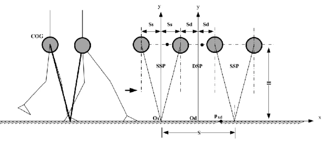
Fig. 1-3: Simplified modeling of biped robot based on method 1. Here and represent half of the distance spent by the COG during the SSP and the DSP respectively.

Because the ZMP is assumed fixed at the center of the stance foot in this work, the left hand

side of Eq. 1-2 will be equal to zero. Consequently, the COG trajectory motion during SSP

can be denoted by

= ( ) + (− ) _Eq._1-3

where , are constants which can be obtained from the boundary conditions, and

= Eq. 1-4

In similar manner, the relationship between ZMP and COG trajectories during the DSP can be expressed as

= − ̈ Eq. 1-5

where denotes the position of COG during DSP; ZMP trajectory can be assumed as

= / _Eq._1-6

where refers to a constant that governs the walking parameters of the biped walking. Then,

we can get the following equation

= ( ) + ( ) _Eq._1-7

(9)

= (1/ − 1)/ _Eq._1-8

To ensure continuous acceleration at the transition moment of the two phases, it is necessary

that ( ̈ = ̈ ) at this moment. Thus, by substituting = − , = in Eq. 1-2 and

Eq. 1-5 we can obtain

+ = Eq. 1-9

If one select and as two independent variables, can be get from Eq. 1-9.

One of the important points lost in the above work is how to determine the suitable DSP time

that corresponds with parameters , and ; selection of the SSP and the DSP time is not

arbitrary to ensure continuous dynamic response. This will be answered in the next method.

1.1.1.2 Method 2: LIPM and LPM-based method [Shi06]

In this method, an inverted pendulum is considered in the SSP and the same equations of the previous method we get; whereas, a linear pendulum mode LPM can be used for modeling the

biped during the DSP as shown in Fig. 1-4. This method was suggested by Shibuya et al.

[Shi06] to relate the ZMP linearly to the COG trajectory. Interestingly, the same Eq. 1-5 is

obtained during the DSP with motion frequency

(10)

Fig. 1-4: Simplified modeling of the biped based on Method 2

with notations shown in Fig. 1-4. Comparing the two mentioned methods (please see Fig. 1-3

and Fig. 1-4), it can be noted that

=(1 − )

2 Eq. 1-11

with denotes a parameter that governs the biped walking, as we will see, and is the step length. In addition

=

2 Eq. 1-12

As a result, we can obtain

= 1 − _Eq._1-13

And the position of the ZMP can be calculated as

= / = /(1 − )

Eq. 1-14

which is the same equation provided by [Shi06]. By comparing Eq. 1-8 and Eq. 1-10, and

substituting Eq. 1-13, we can get

= (1 − ) / _Eq._1-15

which is the same equation obtained in [Shi06]. Therefore, the two methods are equivalent and can give the same results.

Remark 1-1. The correspondent value of the time of DSP ( ) that satisfies the constraint

and continuity equation can be calculated as [Shi06]

= 1

(0) ( ) + ̇ ( ) ̇ ( ) (0) + ̇ ( )

Eq. 1-16

Remark 1-2. . From Eq. 1-13, we can notice the relationship between the parameter and the

parameter . As a result, a relationship between the parameter and the time of DSP ( )

(11)

Remark 1-3. Following the work of [Zhu03], it is possible to consider the constraint

relationship between the angle of the virtual pendulum ( ) and the coefficient of friction ( )

as follows.

0 ≤ ≤ _Eq._1-17

From Fig. 1-4, we can obtain

0 ≤

2 ≤ Eq. 1-18

By selecting the values of and , a suitable value of that satisfies Eq. 1-18 can be chosen.

In brief, we can summarize the procedure for determining the COG trajectory of the biped during the one-step walking as follows:

1. Determine the position of the COG of the biped robot. This depends on the mechanical design of the biped robot. Most researchers have tried to make the COG close to the COG position to simplify the calculations.

2. From Eq. 1-18, select the suitable values of and .

3. From Eq. 1-16, determine the correspondent value of ; the step time and the swing

time can be determined as ⁄0.2 and (0.8 0.2⁄ ) respectively.

4. Using Eq. 1-3 and Eq. 1-7 and their 1st and 2nd derivatives, the motion of COG of the

biped robot can be generated efficiently.

1.1.1.3 Method 3 [Van08]

This method suggests describing a suitable COG acceleration during the DSP satisfying continuous conditions at the transition instance. Vanderborght [Van08] suggested that two types of functions could be employed for this purpose. A linear acceleration at the DSP can be adopted to connect the previous SSP and the next one. However, a large computation can be arisen. Consequently, the author suggested the same acceleration of the SSP can be used but with a negative sign. We will just display the equations required for the acceleration, velocity and the position of the COG trajectory during DSP. For details, we refer to the mentioned reference. We do not mention the case of the SSP because a simplified model of the inverted pendulum can be used during this phase.

̈ ( ) = − ̈ ( ) = −( (− ) + ( )) _Eq._1-19

(12)

( ) = − (− ) + ( ) + ( ̇ ( ) + ( − )) +

+ + ( ) Eq. 1-21

One of the disadvantages of this method is the discontinuity in the position of the COG. This can be solved by modifying the time of the double support phase to guarantee the continuity.

This can coincide with the two previous methods in the selection of suitable in order to

guarantee continuous COG.

Remark 1-4. All the mentioned methods above (1, 2 and 3) need compensation of the ZMP

error due to approximation of the biped robot to pendulum model; the compensation technique will be explained in details later.

1.1.2 Foot trajectory

It is noticed that higher order trajectory may lead to oscillation and overshoot [Gua05]. Therefore, it is desirable to use less order polynomials represented by piecewise spline functions to get the desirable dynamic performance for the biped robot. Huang et al. [Hua99, Hua01] have employed piecewise cubic spline functions for interpolation of the foot trajectory. However, the authors have not assumed zero acceleration where the swing foot becomes flat on the ground (initial full contact). Therefore, Guan et al. [Gua05] have suggested employing fourth order spline functions at the end segments with cubic spline functions for the intermediate segments to guarantee the zero constraint conditions at the end points. Depending on walking patterns 1 and 2, four cases are possible to be studied in order to see some differences of these walking patterns and the effect of impact from kinematics point view.

1.1.2.1 Case 1

In this case, the foot motion will depend on walking pattern 1; the foot is level to the ground

(13)

Fig. 1-5: Foot trajectory for (a) cases 1 and 2 (b) cases 3 and 4.

1.1.2.1.1 The imposed constraint conditions  x-axis :

6 ( 1) = − , 6( 2) = , 6( 3) = ̇ ( ) = ̇ ( ) = 0, ̈ ( ) = ̈ ( ) = 0

Eq. 1-22

where denotes the x-coordinate of the ankle joint, ( , ) is assumed a desired point

should be crossed; it could be the maximum coordinate of the obstacle, = 0, = +

and = + . with represent the time required to cross the obstacle.

In addition to three blending conditions at = ; thus, we have 10 boundary and blending

conditions.  y-axis:

6 ( 1) = 0, 6( 2) = , 6( 3) = 0 ̇ ( ) = ̇ ( ) = 0, ̈ ( ) = ̈ ( ) = 0

Eq. 1-23

where denotes the y-coordinate of the ankle joint.

conditions.

1.1.2.1.2 The proposed piecewise spline functions

Since we have seven boundary conditions for each coordinate, 6-degree polynomial is needed to satisfy these boundary conditions; the blending conditions are important in case of piecewise polynomials. To avoid high oscillated degree polynomials, we can use 4-4 piecewise polynomials (splines) to satisfy the ten boundary and blending conditions, as described below.

(14)

( ) = ( − ) ( ≤ ≤ )

Eq. 1-24

Where Fi (.) represents or .

Remark 1-5. If we intend to use a piecewise spline functions for a trajectory that consists of

two end conditions without intermediate point, it is necessary to select some intermediate point to connect these two segmented polynomials; for details refer to [Gua05].

1.1.2.2 Case 2

The same walking pattern of case 1 is used but with impact at landing, sees Fig. 1-5 (a).

Therefore, the constraint conditions will be as follows.

1.1.2.2.1 The imposed constraint conditions  x-axis :

6 ( 1) = − , 6( 2) = , 6( 3) = ̇ ( ) = ̈ ( ) = 0

Eq. 1-25

conditions.

Remark 1-6. In effect, we have tried to connect the above constraint conditions using 3-3

piecewise spline functions, and 4 degree polynomial separately, but deformation of the trajectory would occur close to the instance of heel strike. Therefore, to get a feasible

trajectory to be compared with other cases, we released the intermediate point at = for x-

trajectory only; thus, we have four boundary conditions.  y-axis:

6 ( 1) = 0, 6( 2) = , 6( 3) = 0 ̇ ( ) = ̈ ( ) = 0

(15)

In addition to three blending conditions at = ; thus, we have also 8 boundary and blending conditions.

1.1.2.2.2 The proposed piecewise spline functions  x- axis

Due to reduction of boundary conditions of x- trajectory (4 boundary conditions); a 3 polynomials could directly be used to satisfy these conditions.

6( ) = 1( − 1) ( 1≤ ≤ 3) 3

=0

Eq. 1-27

 y-axis

We need 3-3 piecewise splines to satisfy the 8 boundary and blending conditions.

( ) = ( − ) ( ≤ ≤ )

Eq. 1-28

where Fi (.) represents .

1.1.2.3 Case 3

This case adopts walking pattern 2 described in Section 2.1 for trajectory generation of feet (see Fig. 1-5 (b)). As we will see in constraint conditions, the foot lands on the ground at heel strike without impact (zero velocity and acceleration). Here philosophy of foot trajectory will change due to rotation of the feet as arcs during the DSP. Thus, finding the feet trajectory (x and y coordinates rather than foot orientation) during the DSP will be easy inspired from mathematical formulae of arcs, whereas spline functions will be applied during the SSP. Piecewise spline functions will be used to generate trajectory of foot orientation during the complete gait cycle; the details are as follows.

1.1.2.3.1 Rear foot trajectory during the period ≤ ≤ (the foot will be in the rear

position)

= − + cos( ) , ̇ = − sin( ) ̇ , ̈ = − sin( ) ̈ +

(16)

= sin( ) , ̇ = cos( ) ̇ , ̈ = (cos( ) ̈ − sin( ) ̇ ) _Eq._1-30

1.1.2.3.2 Swing foot trajectory during the period ≤ ≤

The possible constraint conditions of the swing ankle joint are as follows:  x-axis : 6(0)= − + 7 cos 7(0) , 6( )= , 6( )= − 7+ 7 cos 7( ) − ̇ (0) = − sin( (0)) ̇ (0), ̇ ( ) = − sin( ( ) − ) ̇ ( ) ̈ (0) = − sin (0) ̈ (0) + cos (0) ̇ (0) ̈ ( ) = − (sin( ( ) − ) ̈ ( ) + cos( ( ) − ) ̇ ( ) ) Eq. 1-31

In addition to 3 blending conditions at = ( = − ).

 y-axis 6 (0)= 7 sin 7(0) , 6( )= , 6( )= 7 sin 7( )− ̇ (0) = cos( (0)) ̇ (0), ̇ ( ) = cos( ( ) − ) ̇ ( ) ̈ (0) = (cos (0) ̈ (0) − sin (0) ̇ (0) ) ̈ ( ) = (cos( ( ) − ) ̈ ( ) − sin( ( ) − ) ̇ ( ) ) Eq. 1-32 where = − .

In addition to three blending conditions at = .To satisfy the boundary conditions

(position, velocity and acceleration) of the swing foot with the intermediate point ( , )

which represents the obstacle location, a 6th degree polynomial is needed for each coordinate

( , ) for the swing foot. Instead of using 6th degree polynomial which could lead to more

oscillations, we have used piecewise spline functions with less oscillation. Because we have 10 boundary and blending conditions including the continuity condition (velocity and

acceleration) at the intermediate point, it is possible to use two 4th spline functions to satisfy

(17)

( ) = ( ) 0 ≤ ≤

( ) = ( − ) ≤ ≤

Eq. 1-33

where (. ) represents or coordinate for swing ankle. Briefly, after substituting the

boundary and blending conditions, a linear system of 10 equations can be obtained by which

the constant coefficients of Eq. 1-33 can be found easily.

1.1.2.3.3 Front foot trajectory during the period ≤ ≤ (the foot will be in the

front position)

= − − + cos( − ) , ̇ = − sin( − ) ̇ _Eq._1-34

̈ = − (sin( − ) ̈ + cos( − ) ̇ ) _Eq._1-35

= sin( − ) , ̇ = cos( − ) ̇ , _Eq._1-36

̈ = (cos( − ) ̈ − sin( − ) ̇ ) _Eq._1-37

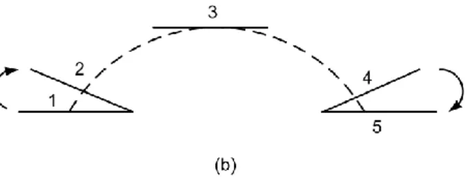
1.1.2.3.4 Orientation trajectory of foot during gait cycle (Trajectory of foot angle) Since the swing foot will impact the ground at instance of heel strike with zero velocity and acceleration; we should divide the angle-foot trajectory into two trajectories as follows.

 Foot angle during the time ₁ ≤ ≤ 4

The imposed constraint conditions

q (t ) = π, q (t ) = q , q (t ) = q

q̇ (t ) = q̇ (t ) = 0

q̈ (t ) = q̈ (t ) = 0

Eq. 1-38

In addition to the three blending conditions at time t ; thus 4-4 spline functions could be used to find all unknowns.

(18)

( ) = ( − ) ≤ ≤

Eq. 1-39

 Foot angle during the time t₄≤ ≤ t₅

The imposed constraint conditions

q (t ) = q , q (t ) = q, q (t ) = π

q̇ (t ) = q̇ (t ) = 0

q̈ (t ) = q̈ (t ) = 0

Eq. 1-40

In addition to the three blending conditions at time t ; thus 4-4 spline functions could be used to find all unknowns.

( ) = ( − ) ≤ ≤ t

( ) = ( − ) t ≤ ≤

Eq. 1-41

Remark 1-7. Concerning trajectory of foot angle during the time t4≤ ≤ t5, additional

intermediate point has been added at time = t to connect the two piecewise splines

together, see Remark 1-5.

1.1.2.4 Case 4

This case is the same as that of case 3 but without zero velocity and acceleration at instance of

heel strike. The derivation of , foot trajectory during the SSP and the DSP are exactly the

same as that of the latter case; see Eq. 1-34 to Eq. 1-41. However, the foot-angle trajectory

will have different imposed constraint conditions; consequently, new piecewise spline functions will be used. The imposed constraint conditions for the foot angle are

q (t ) = π, q (t ) = q , q (t ) = q , q (t ) = π

q̇ (t ) = q̇ (t ) = 0

q̈ (t ) = q̈ (t ) = 0

(19)

In addition to 6 blending conditions at times t and t₄; consequently, the total boundary and blending conditions are 14. To satisfy the above conditions, 4-3-4 piecewise splines can be used as described in the following equations.

( ) = ( − ) ≤ ≤

Eq. 1-43

Remark 1-8. It is assumed that the walking step starts when the front foot strikes the ground

while the rear foot is in full contact, and it ends when the swing foot becomes in full contact with the ground. However, we have assumed that the start time of each phase is set to zero, consequently shifting every piecewise polynomial function is needed in order to achieve this purpose. It should be mentioned that after finding the COG and foot trajectories, the inverse kinematics is necessary to find the biped joint trajectories. For details, we refer to [Van08].

1.2 A simple algorithm for generating stable biped walking patterns

Despite miscellaneous walking pattern generation and stabilization approaches, it is difficult to find a thorough method that can tune the walking parameters to satisfy the kinematic and dynamic constraints: singularity condition at the knee joint, ZMP constraint, and unilateral contact constraints. Another problem that has been investigated in this section is the generation of foot trajectory during DSP. References [Hua99, Hua01] used piecewise spline functions to approximate the trajectory of the front and rear feet during DSP. It is known that during DSP the front foot rotates about the heel joint while the rear foot rotates about its front tip; therefore, their trajectories can be found easily by trigonometric relationships for arcs rather than approximate spline which can results in deviations in the velocity and acceleration of the feet especially at the transition instances. Therefore the following subsections propose a sufficient algorithm that solves the mentioned problems.

1.2.1 COG Trajectory

Eq. 1-3 and Eq. 1-7 can describe trajectory of biped COG during the SSP and the DSP

respectively.

Remark 1-9. Some of the drawbacks of walking pattern 2 have been described in Chapter 6

(20)

stability/balance problem. Moreover, trajectory planning of walking patterns 2 and 3 could be similar; the difference is that motion the front and rear feet during the walking pattern 2 are simultaneous, while their motion will be consecutive in walking pattern 3. Therefore, the next subsection will describe a novel algorithm for compensating for deviations of ZMP trajectory concerning walking patterns 2 and 3.

1.2.2 Feet trajectory

Subsection 6.1.2.3 describes in details the trajectory of feet for walking pattern 2; the same equations can be used for generating foot trajectory for walking pattern 3 (the difference lies in timing the DSP). In more details for walking pattern 3, the sequences of phase times are

= 0, − = , − = , − = ), whereas for walking pattern 3 they are

= 0, − = /2, − = , − = /2).

1.2.3 Kinematic and dynamic constraints

 Singularity constraint

There could be three reasons which may lead ZMP-based biped robot to walk with bent knees: (a) constraining the COG trajectory to move in constant height, (b) appearance of the difference of shank and thigh angles at the denominator in the inverse kinematics solution. (c) if the DSP is included in the trajectory planning, the constraint control (force control) of the biped could demand the same problem of (b) during solution.

Applying the cosine’s law

Ω = (2 − ) 2⁄

Eq. 1-44

with Ω denotes the angle between the thigh link and the shank link, is the length of the

shank link which is equal to the thigh one, and represents the distance between the ankle joint and the COG joint. To avoid singularity position for the knee joint, it is necessary to satisfy the following condition

−1 < (2 − ) 2⁄ < 1 _Eq._1-45

 Unilateral contact constraints

Please see Eq. 4-54 which can be used to describe unilateral contact constraints during the SSP and the DSP.

(21)

Remark 1-10. Since the biped robot does not have a unique solution during the DSP, we assume a linear transition function for the ground reaction forces of the front foot (right foot) as described in Subsection 4.2.1.3.

 Zero-moment point constraint

− ≤ ≤ 0 for SSP

− ≤ ≤ for DSP

Eq. 1-46

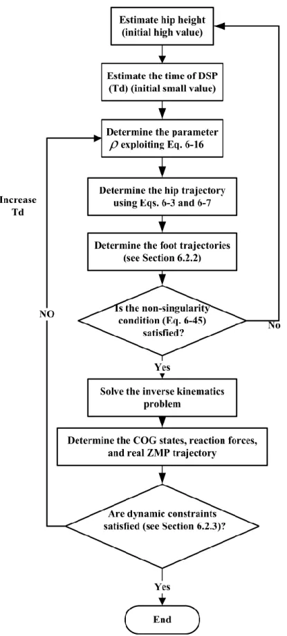
1.2.4 The proposed algorithm

As said previously, the pendulum model is approximate model for biped robot because the real robot is multibody system. In addition the biped mechanism is inherently unstable and has not fixed base. Therefore, to get feasible biped motion, the aforementioned kinematic and

dynamic constraints should be satisfied via modifying the times of the DSP ( ) and the SSP

(increasing the phase times). The distance travelled by the COG during the walking phases will be changed accordingly; this will be clear in the simulation results. The proposed

(22)

(23)

1.3 Simulation results and discussions

The results can be divided into three categories as follows:

1.3.1 Comparison between methods 1, 2 and 3

Following the procedure described in Subsection 1.1.1 for generation of COG trajectory, the

desired (walking) parameters have been used ( = 0.5, = 0.7561 (cases 1 , 2), =

0.7575 (cases 3 , 4), = 0.5 [ ], = 0.125 [ ]). It is noticed that there is clear

relationship between the walking parameter and as expressed in Eq. 1-16. We have

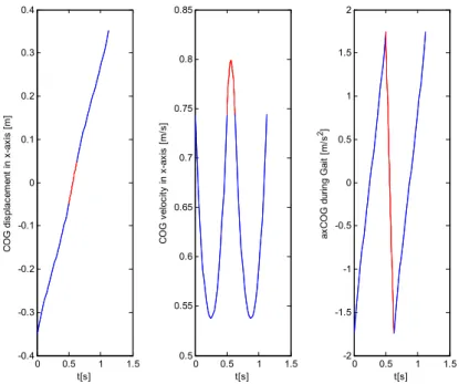
employed the mentioned parameters with methods 1, 2 and 3. Consequently, the COG motion is continuous regarding position, velocity and acceleration, as shown in Fig. 1-7. In effect, the methods 1 and 2 are identical; therefore, we compared between methods 2 and 3. The latter two methods give similar motion. However, Method 2 is more systematic in dealing with the parameters of the biped walking and guaranteeing the constraint and continuity conditions. From Fig. 1-7, it is clear that the SSP encounters deceleration and acceleration sub-phases

sequentially. This can be explained according to Eq. 1-2 where deceleration of the biped

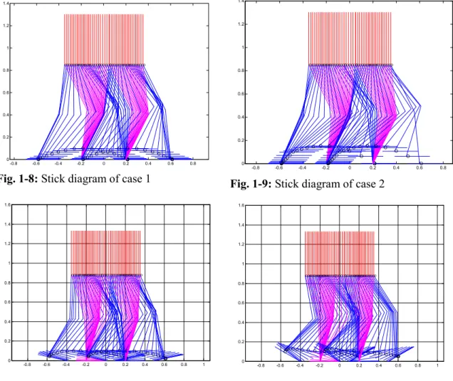
robot can occur until the middle of SSP because the COG position is behind the front stance foot. The next acceleration sub-phase can result from the progression of the COG in front of the stance foot. Another issue that can be noticed is that the motion of the hip link is close in the middle of SSP, as shown in Fig. 1-8 to Fig. 1-11. As aforementioned, the COG of the biped robot will decelerate very slowly at the middle region of the SSP, and then it accelerates slowly near this region.

Fig. 1-7: The position, velocity and acceleration of COG (hip) (Method 2 ----; whereas

Method 3 ). As noted, the two methods have the same results.

0 0.5 1 1.5 -0.4 -0.3 -0.2 -0.1 0 0.1 0.2 0.3 0.4 t[s] C OG d is p lac e m e n t in x -a x is [ m ] 0 0.5 1 1.5 0.5 0.55 0.6 0.65 0.7 0.75 0.8 0.85 t[s] C OG v e loc it y in x -a x is [ m/ s ] 0 0.5 1 1.5 -2 -1.5 -1 -0.5 0 0.5 1 1.5 2 t[s] a x C OG d u ring Ga it [ m/ s 2] _______

(24)

Fig. 1-8: Stick diagram of case 1 _Fig._{1-9: Stick diagram of case 2}

(a) with contact angle of 120. (b) with contact angle of 300. Fig. 1-10: Stick diagram for case 3

(a) Stick diagram of case 4 with contact angle of 120.

(b) Stick diagram of case 4 with contact angle of 300.

Fig.1-11: Stick diagram for case 4

-0.8 -0.6 -0.4 -0.2 0 0.2 0.4 0.6 0.8 0 0.2 0.4 0.6 0.8 1 1.2 1.4 O o O o O o O o O o O o O o O o O o O o O o O o O o O o O o O o O o O o O o O o O o O o O o O o O o O o O o O o O o O o O o O o O o O o O o O o O o O o O o O o O o O o O o O o O o O o O o O o -0.8 -0.6 -0.4 -0.2 0 0.2 0.4 0.6 0.8 0 0.2 0.4 0.6 0.8 1 1.2 1.4 O o O o O o O o O o O o O o O o O o O o O o O o O o O o O o O o O o O o O o O o O o O o O o O o O o O o O o O o O o O o O o O o O o O o O o O o O o O o O o O o O o O o O o O o O o O o O o O o -0.8 -0.6 -0.4 -0.2 0 0.2 0.4 0.6 0.8 1 0 0.2 0.4 0.6 0.8 1 1.2 1.4 1.6 O o O o O o O o O o O o O o O o O o O o O o O o O o O o O o O o O o O o O o O o O o oooooo O o O o O o O o O o O o O o O o O o O o O o O o O o O o O o O o O o O o O o O o O o -0.8 -0.6 -0.4 -0.2 0 0.2 0.4 0.6 0.8 1 0 0.2 0.4 0.6 0.8 1 1.2 1.4 1.6 O o O o O o O o O o O o O o O o O o O o O o O o O o O o O o O o O o O o O o O o O o oooooo O o O o O o O o O o O o O o O o O o O o O o O o O o O o O o O o O o O o O o O o O o -0.8 -0.6 -0.4 -0.2 0 0.2 0.4 0.6 0.8 1 0 0.2 0.4 0.6 0.8 1 1.2 1.4 1.6 O o O o O o O o O o O o O o O o O o O o O o O o O o O o O o O o O o O o O o O o O o OOOOOO O o O o O o O o O o O o O o O o O o O o O o O o O o O o O o O o O o O o O o O o O o -0.8 -0.6 -0.4 -0.2 0 0.2 0.4 0.6 0.8 1 0 0.2 0.4 0.6 0.8 1 1.2 1.4 1.6 O o O o O o O o O o O o O o O o O o O o O o O o O o O o O o O o O o O o O o O o O o oooooo O o O o O o O o O o O o O o O o O o O o O o O o O o O o O o O o O o O o O o O o O o

(25)

1.3.2 Gait Patterns based on foot trajectory

In this study, four cases of foot trajectory with different boundary conditions were compared

as detailed in Section 1.1.2. The characteristics (advantages and disadvantages) of these cases

are detailed in Tab. 1-1.

Tab. 1-1: The characteristics of foot trajectory according to the four simulated cases.

Case No Characteristics

1  The foot is level to the ground.

 The maximum hip height is 85 [mm]; increasing this value could result in singularity at knee joint.

 Due to zero velocity and acceleration at end conditions, the swing foot moves very slowly at these ends; this can lead more energy consumption especially at heel strike [Van08].

 Due to the latter point, relatively messing configuration of swing leg at the end of swing phase; see Fig. 1-8.

2  The foot is also level to the ground.

 The maximum hip height is 85 [mm]; increasing this value could result in singularity at knee joint.

 There is some change in behavior of foot motion at the end of the swing phase due to free condition (striking the ground with some velocity) at this end. This may explain the uniform configuration of the swing leg at end of this phase, see Fig. 1-9.

 It is difficult to add intermediate point for foot trajectory in x-axis due to the free condition mentioned previously, see Remark 1-6.

3  The foot takes off and strikes the ground with specified angles; see Fig. 1-10 .  Although the biped robot strikes the ground without impact, its configuration can

be improved by modifying landing angle as shown in Fig. 1-10 (a) and (b).

 The foot moves very slowly at the beginning and end of the swing phase due to its zero end conditions.

4  The foot trajectory has the same characteristics as that of case 3 but with some free motion at heel strike due to free impact at this instance; see Fig. 1-11.

1.3.3 Compensation of ZMP deviations using algorithm of Fig. 1-6

All above analyses have been performed without checking whether the ZMP trajectory is still inside the support polygon or not, see Chapter 2 of [Hay14] for more details on this important

(26)

criterion. In this study, we concentrated on walking pattern 2 and 3. In general, the results can be summarized as follows:

 Walking pattern 3 before and after compensation.

We selected initial parameters for our biped model ( = 0.88 , = 0.7557, =

0.125 [ ], = 0.5 [ ]). In effect, these parameters have been selected according to previous

work which deals with suboptimal trajectory planning of the same robot model. The proposed hip height of the biped can violate the singularity condition. Therefore, unreasonable solution can be obtained due to appearance of imaginary numbers. Our suggested algorithm tunes the

mentioned parameters to give stable trajectory for the COG of biped model. Tab. 1-2 shows

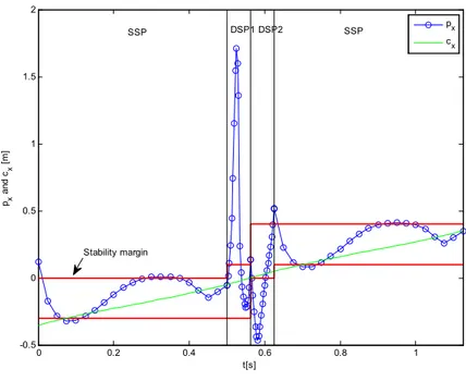
the walking parameters before and after compensation while Fig. 1-12 and Fig. 1-13 show COG and ZMP trajectories before and after tuning respectively.

Tab. 1-2: Tuning of walking parameters

Walking parameters Before

compensation

= 0.88 , = 0.5757, = 0.125 [ ], = 0.5 [ ]

After compensation = 0.86 , = 0.6203, = 0.3 [ ], = 1.2 [ ]

Fig. 1-12: ZMP and COG trajectories before compensation (walking pattern 3)

0 0.2 0.4 0.6 0.8 1 -0.5 0 0.5 1 1.5 2 t[s] px an d c x [ m ] p_x c_x Stability margin DSP1 DSP2 SSP SSP

(27)

Fig. 1-13: ZMP and COG trajectories after compensation (walking pattern 3)

 Walking pattern 2 vs. walking pattern 3.

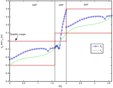
From Fig. 1-14, it could be noted that the ZMP is out of its stability margin at the beginning of the DSP due to rotation of the rear foot instantaneously at the DSP. This instability can be avoided in walking pattern 3 which can guarantee smooth transition or ZMP trajectory and foot rotation. In effect, keeping stance foot fixed at beginning of DSP is necessary to get stable motion.

Fig. 1-14: ZMP and COG trajectories after compensation (walking pattern 2)

0 0.5 1 1.5 2 2.5 -0.5 -0.4 -0.3 -0.2 -0.1 0 0.1 0.2 0.3 0.4 0.5 t[s] px an d c x [ m ] p_x c_x SSP DSP1 DSP2 SSP Stability margin 0 0.5 1 1.5 2 2.5 3 3.5 -0.5 -0.4 -0.3 -0.2 -0.1 0 0.1 0.2 0.3 0.4 0.5 t[s] px a n d cx [ m ] p x c_x Stability margin SSP DSP SSP

(28)

2 Conclusions

 In this report, we have attempted to focus on the smooth transition from the SSP to

the DSP and vice versa. Three methods have been compared for this purpose. The first two methods have exploited the notion of pendulum mode with different strategies. However, it is found that the two mentioned methods can give the same motion of center of gravity for the biped. Whereas, Method 3 has suggested to use a suitable acceleration during the double support phase (DSP) for a smooth transition. Although the Method 3 can give close results as in the former methods, the latter are more systematic in dealing with the walking parameters of the biped robot. The second issue we focus on is the different patterns of the foot trajectory especially during the DSP. The characteristics of foot rotation can improve the stability performance generating uniform configuration.

 The last part of this report concentrates on compensating the ZMP deviations due

to approximate model of LPM. Successful results can be got with walking pattern 3.

 All above methods are offline applied because it uses much iteration to get the

feasible motion for the target biped. The online modified version should be tested and selected carefully as discussed in detail in Chapter 3 of [Hay14].

3 References

[Gua05] Guan, Y.; Yokoi, K.; Stasse, O.; Kheddar, A. On robotic trajectory planning using

polynomial interpolations. In Proc. IEEE Conf. Robotics and Biomimetics, pp. 111-116,

2005.

[Hay 18/4] Al-Shuka, Hayder F. N. Design of walking patterns for zero-momentum point (ZMP)-based biped robots: a computational optimal control approach, Munich, GRIN Verlag

(2018) https://www.grin.com/document/434367.

[Hay13/1] Al-Shuka, Hayder F. N; Corves, B. On the walking pattern generators of biped

robot. Journal of Automation and Control, Vol.1,No. 2, pp.149-156 (March 2013)

http://www.joace.org/uploadfile/2013/0506/20130506045849456.pdf.

[Hay13/2] Al-Shuka, Hayder F. N; Corves, B.; Zhu, Wen-Hong. On the dynamic optimization

of biped robot. Lecture Notes on Software Engineering, Vol. 1, No. 3, pp. 237-243 (June

2013) https://pdfs.semanticscholar.org/856d/42547334681b2afe79067d52fc9b0103d8ee.pdf.

[Hay13/3] Al-Shuka, Hayder F. N; Corves, B.; Vanderborght, B.; Zhu, Wen-Hong. Finite

difference-based suboptimal trajectory planning of biped robot with continuous dynamic response. International Journal of Modeling and Optimization, Vol.3, No. 4, pp.337-343

(August 2013) http://www.ijmo.org/papers/294-CS0019.pdf.

[Hay14/1] Al-Shuka, Hayder F. N; Corves, B.; Zhu, Wen-Hong; Vanderborght, B. A Simple

algorithm for generating stable biped walking patterns. International Journal of Computer

Applications, Vol. 101, No. 4, pp. 29-33 (Sep. 2014)

(29)

[Hay14/2] Al-Shuka, Hayder F. N; Corves, B.; Zhu, Wen-Hong. Dynamic modeling of biped

robot using Lagrangian and recursive Newton-Euler formulations. International Journal of

Computer Applications, Vol. 101, No. 3, pp. 1-8 (Sep. 2014)

http://citeseerx.ist.psu.edu/viewdoc/download?doi=10.1.1.800.2667&rep=rep1&type=pdf. [Hay14/3] Al-Shuka, Hayder F. N; Allmedinger, F; Corves, B.; Zhu, Wen-Hong. Modeling,

stability and walking pattern generators of biped robots: a review. Robotica, Cambridge

Press, Vol. 32, No. 6, pp. 907-934 (Sep. 2014) https://doi.org/10.1017/S0263574713001124.

[Hay14/4] Al-Shuka, Hayder F. N; Corves, B.; Zhu, Wen-Hong. Function approximation

technique-based adaptive virtual decomposition control for a serial-chain manipulator.

Robotica, Cambridge Press, Vol. 32, No. 3, pp. 375-399 (May 2014)

https://doi.org/10.1017/S0263574713000775.

[Hay14] Al-Shuka, Hayder F. N. Modeling, walking pattern generators and adaptive control

of biped robot. PhD Dissertation, RWTH Aachen University, Department of Mechanical

Engineering, IGM, Germany (2014) http://publications.rwth-aachen.de/record/465562.

[Hay15] Al-Shuka, Hayder F. N; Corves, B.; Vanderborght, B.; Zhu, Wen-Hong.

Zero-moment point-based biped robot with different walking patterns. International Journal of

Intelligent Systems and Applications, Vol. 07, No. 1, pp. 31-41 (2015)

https://www.researchgate.net/publication/267865541_Zero-Moment_Point-Based_Biped_Robot_with_Different_Walking_Patterns.

[Hay16] Al-Shuka, Hayder F. N; Corves, B.; Zhu, Wen-Hong; Vanderborght, B. Multi-level

control of zero moment point-based biped humanoid robots: a review. Robotica, Cambridge

Press, vol. 34, No. 11, pp. 2440-2466 (2016) https://doi.org/10.1017/S0263574715000107.

[Hay17/1] Al-Shuka, Hayder F. N. Stress distribution and optimum design of polypropylene

and laminated transtibial prosthetic sockets: FEM and experimental implementations.

Munich, GRIN Verlag (2017) https://www.grin.com/document/385910.

[Hay17/2] Al-Shuka, Hayder F. N. An overview on balancing and stabilization control of

biped robots. Munich, GRIN Verlag (2017) https://www.grin.com/document/375226

[Hay18/1] Al-Shuka, Hayder F. N.; Song, R. On low-level control strategies of lower

extremity exoskeletons with power augmentation. The 10th IEEE International Conference on

Advanced Computational Intelligence, Xiamen, China, pp. 63-68 (2018)

DOI:10.1109/ICACI.2018.8377581.

[Hay18/2] Al-Shuka, Hayder F. N.; Song, R. On high-level control of power-augmentation

lower extremity exoskeleton: human walking intention. The 10th IEEE International Conference on Advanced Computational Intelligence, Xiamen, China, pp. 169-174 (2018)

DOI: 10.1109/ICACI.2018.8377601.

[Hay18/3] Al-Shuka, Hayder F. N. On local approximation-based adaptive control with

applications to robotic manipulators and biped robot. International Journal of Dynamics and

Control, Springer, Vol. 6, No. 1, pp. 393-353 (2018)

https://doi.org/10.1007/s40435-016-0302-6.

[Hay19] Al-Shuka, Hayder F. N.; Song, R. Decentralized Adaptive Partitioned

Approximation Control of Robotic Manipulators. In: Arakelian V., Wenger P. (eds),

ROMANSY 22 – Robot Design, Dynamics and Control. CISM International Centre for Mechanical Sciences (Courses and Lectures), vol 584. Springer, Cham (2019)

(30)

[Hua01] Huang, Q.; Yokoi, K.; Kajita, S.; Kaneko, K.; Arai, H.; Koyachi, N.; Tanie, K.

Planning walking patterns for a biped robot. IEEE Transactions on Robotics and

Automation:17(3), 280 – 289, 2001.

[Hua99] Huang, Q., Kajita, S., Koyachi, N.; Kaneko, K. A high stability, smooth walking

pattern for a biped robot. IEEE International conference on Robotics and Automation, vol. 1,

Detroit, MI, pp.65-71 (May 1999).

[Kaj96] Kajita, S.; Tani, K. Experimental study of biped dynamic walking. IEEE, Control Systems: 16 (1),13-19, 1996

[Kud03] Kudoh, S.; Komura, T. C2 continuous gait-pattern generation for biped robots. In

Proc.2003 IEEE/RSJ Intelligent Robots and Systems, vol.2, pp. 1135-1140, 2003.

[Mu03] Mu, X.; Wu, Q. Synthesis of a complete sagittal cycle for a five-link biped robot. Robotica: vol. 21, pp. 581-587, 2003.

[Shi06] Shibuya, M., Suzuki, T.; Ohnishi, K. Trajectory planning of biped robot using linear

pendulum mode for double support phase. In Proc. IECON 2006-32nd Annual Conf. IEEE

Industrial Electronics, pp.4094-4099 (2006).

[Tan03] Tang, Z.; Zhou, C.; Sun, Z. Trajectory planning for smooth transition for a biped

robot. IEEE International conference on Robotics and Automations, vol. 2, pp. 2455-2460

(2003).

[Van08] Vanderborght, B.; Ham, R. V.; Verrelst, B.; Damme, M. V.; Lefeber, D. Overview

of the Lucy project: Dynamic stabilization of a biped powered by pneumatic artificial muscles. Advanced Robotics: 22 (10), 1027-1051, 2008.

[Vuk72] Vukobratovic, M.; Stepanenko, J. On the stability of anthropomorphic systems. Mathematical Biosciences: 15 (1-2), 1–37, 1972.

[Zhu03] Zhu, C.; Kawamura, A. Walking principle analysis for biped robot with ZMP

concept, friction constraint, and inverted pendulum mode. In Proc. 2003 IEEE/RSJ Intl.

Walking pattern generators of biped robots using a linear pendulum model with compensated ZMP

HAL Id: hal-02116967

https://hal.archives-ouvertes.fr/hal-02116967

Hayder Al-Shuka, Burkhard Corves, Bram Vanderborght, Wen-Hong Zhu

To cite this version:

Walking pattern generators of biped robots using a

linear pendulum model with compensated ZMP

Contents