HAL Id: hal-02924113
https://hal.archives-ouvertes.fr/hal-02924113
Submitted on 21 Nov 2020
HAL is a multi-disciplinary open access
archive for the deposit and dissemination of sci-entific research documents, whether they are pub-lished or not. The documents may come from teaching and research institutions in France or abroad, or from public or private research centers.
L’archive ouverte pluridisciplinaire HAL, est destinée au dépôt et à la diffusion de documents scientifiques de niveau recherche, publiés ou non, émanant des établissements d’enseignement et de recherche français ou étrangers, des laboratoires publics ou privés.
Variability of Satellite Sea Surface Salinity Under
Rainfall
Alexandre Supply, Jacqueline Boutin, Gilles Reverdin, Jean-Luc Vergely,
Hugo Bellenger
To cite this version:
Alexandre Supply, Jacqueline Boutin, Gilles Reverdin, Jean-Luc Vergely, Hugo Bellenger. Variability of Satellite Sea Surface Salinity Under Rainfall. Satellite Precipitation Measurement, V. Levizzani, C. Kidd., D. B. Kirschbaum, C. D. Kummerow, K. Nakamura, F. J. Turk, Eds., Springer Nature, Cham, Advances in Global Change Research, pp.1155-1176, 2020, �10.1007/978-3-030-35798-6_34�. �hal-02924113�
1.1 V
ARIABILITY OF SATELLITE SEA SURFACE SALINITY
UNDER RAINFALL
Alexandre Supply1, Jacqueline Boutin1, Gilles Reverdin1, Jean-Luc Vergely2 and Hugo
Bellenger3,4.
Abstract Two L-Band (1.4GHz) microwave radiometer missions, the Soil Moisture and
Ocean Salinity (SMOS) and the Soil Moisture Active and Passive (SMAP) missions, currently provide salinity measurements in the first centimeter below the sea surface. At this depth, salinity variability at hourly temporal scales is dominated by the impact of precipitation. The dependency of the salinity freshening with the instantaneous rain rate (RR) observed between 50°S and 50°N, with SMOS and SMAP salinities, is very similar.
We investigate the influence of rain history on salinity anomalies. By using rain rates retrieved from several microwave satellites measurements including Advanced Microwave Scanning Radiometer 2 (AMSR-2), and Special Sensor Microwave Imager Sounder 17 (SSMIS-17 and SSMIS-16) and by taking advantage of their different crossing times, we estimate the temporal cross-correlation function between salinity freshening and rain rate for different time lags in various tropical and high latitudes regions. Whatever the region, the magnitude of the salinity anomaly associated with precipitation is dominated by the instantaneous RR for each area. The apparent correlation between salinity anomaly and rain history can be explained by RR auto-correlation.
The relationship between salinity anomaly (∆S) and RR is then investigated in six regions, with RR provided using three different algorithms (the Unified Microwave Ocean Retrieval Algorithm (UMORA), the Goddard profiling algorithm (GPROF) and Integrated MultisatellitE Retrievals for GPM (IMERG)). Differences in RR distribution between the various algorithms lead to differences of up to a factor 2 in ∆S versus RR slopes. For a given RR product, we also observe that part of the variability in ∆S versus RR relationships is related to the variability in wind speed regimes as detected by SMAP wind speed.
1 Sorbonne Université, CNRS, IRD, MNHN, Laboratoire d'Océanographie et du Climat: Expérimentations et Approches Numériques (LOCEAN), IPSL, 75005 Paris, France.
2 ACRI-st, Guyancourt, France.
3 Laboratoire de Météorologie Dynamique (LMD), IPSL, CNRS, Sorbonne Université, Ecole Normale Supérieure, Ecole Polytechnique, 75005 Paris, France.
1.1.1 Introduction
Since 2010, the Soil Moisture and Ocean Salinity (SMOS; Kerr et al., 2010) mission provides the longest record of Sea Surface Salinity (SSS) from space, with a spatial resolution of ~50km4. Since 2015, the Soil Moisture Active and Passive (SMAP; Piepmeier et al., 2017)
performs measurements at a similar spatial resolution. Hence, during the last 3 years, the complementarity of the spatio-temporal sampling by the two instruments provides the opportunity to improve the spatial and temporal coverage of salinity measurements from space and to reduce the mean time lag between two salinity estimates in a given pixel.
Although satellite sea surface salinity (SSS) measurements are slightly noisier than in-situ SSS measurements, recent reprocessing of SMOS and SMAP SSS estimates provide very realistic SSS variability with a spatio-temporal resolution not accessible from in situ measurements only (Tang et al. 2017; Boutin et al. 2018). They are of special interest for studying synoptic SSS variability at scales not resolved by Argo measurements, roughly less than 600km and less than one month (e.g. Boutin et al. 2015). In particular, satellite SSS provides new insights into links between river discharge and interannual variability of SSS, e.g. in the Gulf of Mexico (Fournier et al. 2016), and in the western equatorial Atlantic Ocean (Fournier et al. 2017a). At weekly and small spatial scales, strong interaction between fresh
river plumes, currents and mesoscale eddies have been evidenced by Fournier et al. (2016) and Fournier et al. (2017b) in the Gulf of Mexico and Bay of Bengal, respectively.
Rainfall influences salinity at various scales. During a year, ITCZ rainfall and Ekman dynamics lead to the displacement of a significant amount of freshwater, greatly reducing salinity in rainy areas but also in non-rainy areas by Ekman transport (Yu, 2015; Hasson et al. 2018). Abe et al. (2018) show that accumulation of rain may induce the formation of low salinities eddies with low salinity reaching 70m depth. These studies, which provide information on various phenomena that impact SSS at temporal scales longer than typically one month, are an important background to consider when investigating the effect of rain rate (RR) on SSS at smaller temporal scales. A better understanding of salinity freshening due to rain is needed to improve the interpretation of satellite salinity. Actually, rain events may induce large differences (>1pss) between the first upper centimeter of the ocean and a few meters depth (Henocq et al. 2010, Reverdin et al. 2012). Current ocean general circulation models usually do not include a detailed description of the processes involved in the upper centimeters depth (Bellenger et al. 2017), so that a rain correction should be first applied to the satellite salinity before they can be confronted with ocean model simulations at several tens of centimeters or several meters depth.
After a rain event, salinity is generally quickly restored (on the order of a few hours) to a level close to the one observed before the rain event (Wijesekera et al. 1999; Soloviev et al. 2002; Reverdin et al. 2012; Drushka et al. 2016). However, in some cases, fresh lenses have been observed with a persistence time close to 24h (Walesby et al. 2015; Dong et al. 2017, Pei et al. 2018). Fresh lens emergence and their spatial and temporal evolution are not well understood (air-sea fluxes of heat and momentum, advection, upper-ocean mixing, etc.). Recent studies succeed to simulate rain-induced fresh lens formation and life cycle by using one-dimensional water column models, the Generalized Ocean Turbulence Model (GOTM; Drushka et al., 2016) or a prognostic model (Bellenger et al., 2017). In these cases, duration of freshwater cool lens is estimated as function of windspeed (WS) and maximum RR. With a
4Estimated as the diameter of the equivalent circle, centered on a Grid Point, where SSS is retrieved. The area of the equivalent
circle is equal to the mean area of the footprint ellipses of the brightness temperatures (Tb) entering in the SSS retrieval. However, given that the SMOS noisiest Tb are the ones having the lowest resolution, the effective SMOS SSS resolution is likely between 43km (the mean diameter in the Alias Free Field Of View) and 50km.
maximum RR of 20mm. h%&,a fresh lens may persist less than 2 hours in high WS (10m. s%&)
conditions and up to 7 hours in the low WS (1m. s%&) case (Bellenger et al., 2017). However,
these studies are limited to very local scale and have been validated with a limited number of in situ measurements. To predict the influence of rain on salinity, the Rain Impact Model (RIM) applies a one-dimensional turbulent diffusion model from Asher et al. (2014) considering a rain history from the past 24 hours that was calibrated using a few rain events observed with the Surface Salinity Profiler (SSP) instrument during the Kilo Moana 2011 cruise (Asher et al. (2014)).
Based on satellite observations, a strong correlation between SSS negative anomalies (∆)) and RR at short temporal (less than one hour) scales have been reported by several studies (see a review in Boutin et al. 2016). Dependency of SSS freshening with RR has a similar order of magnitude to the ones obtained by Schlussel et al. (1997) with a surface renewal model of the molecular diffusion layer, 0.05mm for salinity, likely because rain mixing affects salinity in the first centimeters of the surface ocean (Ho et al. 2000; Zappa et al. 2009).
Supply et al. (2017) focuses on the relationship between ∆) and RR in the Inter Tropical Convergence Zone area without considering the potential influence of WS and RR history on the relationship despite the link shown with in-situ measurements. Santos-Garcia et al. (2014), use the RIM model fitted to Aquarius satellite measurements to relate Aquarius ∆) to rain accumulation during the previous 24h. However, given the temporal under sampling of SSS measured by a single satellite mission (at least 12h), these studies do not allow one to estimate precisely the hourly evolution of ∆) associated with a rainy event. Thus, to date, a clear freshening signature remaining at the sea surface a few hours after a rain event was not demonstrated in satellite data. We investigate here the role of RR history on SSS anomalies by using several RR satellites combined with SMOS and SMAP data. Models and in-situ measurements indicate that the relationship between RR and ∆) is influenced by WS. We also study this dependency with satellite measurements.
Our study region covers all the oceans between 50°S and 50°N, after removing periods and areas with SSS variability driven by non-rainy processes. A better understanding of the link between RR and ∆) will also benefit satellite RR estimation. Validation of RR measurements over ocean is hindered by the low number of measurements, especially at high latitudes and the difficulty of comparing punctual in-situ and spatially integrated satellite measurements. Compared with RR satellites, SMOS and SMAP SSS measurements have very close spatial resolution and offer an alternative method to complement the rainfall monitoring. We analyze the possibility of using both satellites to assess different RR products.
In section 1.1.2, we introduce data and methods. In section 1.1.3, results are detailed: 1/ intercomparison of RR and SSS products; 2/ imprint of RR history on SSS anomaly; 3/ variability of ∆S/RR relationship and influence of WS and rain product. In section 1.1.4, we discuss the results and perspectives of this study.
1.1.2 Data & method
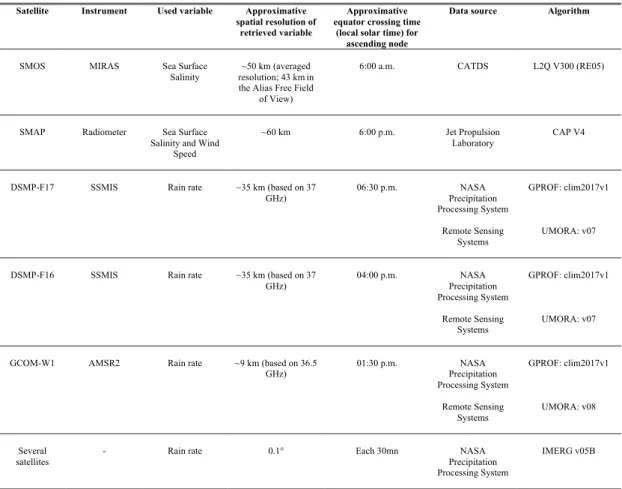
SSS, WS and RR data used in this study are summarized in Table 1.
1.1.2.1 Salinity and wind speed data
The SMOS mission carries an L-band Microwave Interferometric Radiometer with Aperture Synthesis (MIRAS) from which SSS measurements are retrieved. It provides SSS from space since 2010 (Reul et al. 2014). We consider only SMOS retrieved SSS at +/-400km from the center of the swath, which are less noisy. SMOS has a revisit time between 3 and 5 days and follows a Sun synchronous orbit with a local equator crossing time at 6:00 a.m. on the
ascending node. SMAP provides SSS from space since April 2015. The SMAP swath is 1000 km with a shorter revisit time (between 2 and 3 days). It crosses the Equator at the same local time as SMOS but in the opposite phase, near 6:00 a.m. for descending orbits and near 6:00 p.m. for ascending orbits.
In this study, we use the following level 2 SSS. SMOS SSS are corrected from land-sea contamination and from seasonal latitudinal systematic effects as described in (Boutin et al. 2018) and are available at CATDS (Centre Aval de Traitement des Données SMOS) (SMOS CPDC L2Q products (CATDS 2017)). SMAP SSS are from the L2B version 4 product from JPL (Fore et al. 2017). Satellite SSS are oversampled on an Equal-Area Scalable Earth Grid (EASE) grid of 25km spacing for SMOS and on a swath grid of 25km spacing for SMAP. The effective spatial resolution of these SMOS and SMAP level 2 SSS are quite similar, close to 60km for SMAP and 50km for SMOS.
Erroneous SMOS L2Q SSS are removed based on the minimum and maximum acceptable values provided in the files (Vergely and Boutin 2017). We also remove SSS values identified as non-valid during the retrieval process before the application of the bias removal process (Vergely and Boutin 2017) and SSS values very different (difference larger than 3pss) from a nearby SSS flagged as valid. For SMAP, we use SSS data flagged as valid.
SMOS and SMAP SSS are retrieved using a maximum likelihood approach. For both products, an SSS uncertainty is derived by taking the observed mismatches between observed and modelled brightness temperatures (Tbs) (e.g. like in RFI polluted areas) into account (Boutin et al. 2018; Fore et al. 2017). In our study we only consider SMOS or SMAP SSS with uncertainty lower than 0.8pss.
We use WS provided in the SMAP files, assuming that the constant 40° incidence angle of SMAP and its rotating antenna would provide a WS with a more conservative error than the SMOS estimate that is likely dependent on the geometry in the SMOS field of view and that covers incidence angles from 0 to ~60° while horizontal-vertical polarization contrasted signature of roughness is only expected at high incidence angles. The WS retrieved by the SMAP CAP v4 retrieval algorithm uses National Centers for Environmental Prediction Global Forecast System (NCEP GFS) ancillary WS with an error of 1.5m s-1 (Fore et al. 2017).
All SSS and WS data are interpolated for each day (ascending and descending orbits separately) on a regular grid of 0.2°x0.2° before deriving SSS anomalies from SMOS (∆)+,-+)
and SMAP (∆)+,./). 1.1.2.2 Rain rate data
Our study takes advantage of the satellite constellation of Global Precipitation Measurements (GPM) project (Hou et al., 2014), dedicated to providing the best possible coverage for monitoring rainfall (Kidd and Huffman, 2011), with RR from three different algorithms: Unified Microwave Ocean Retrieval Algorithm (UMORA; Hilburn and Wentz, 2008; Wentz et al. 2012; Wentz et al. 2014), The Goddard Profiling scheme (GPROF; Kummerow et al. 1996; GPM Science Team, 2016, 2017a and 2017b) and the Integrated Multi-satellitE Retrievals for GPM (IMERG; Huffman et al, 2018). GPROF uses a Bayesian approach and cloud resolving models to extract rain information. UMORA simultaneously retrieves sea surface temperature, surface wind speed (in case of no rain), columnar water vapor, columnar cloud water, and surface rain rate from a variety of passive microwave sensors, after a very careful intercalibration of the various sensors (Hilburn and Wentz, 2008). It uses an empirical relationship between cloud water liquid path, RR and rain column height. These two different algorithms make different microphysical assumptions, cloud and rain partitioning and rain column height. Previous studies have shown that with temporal and spatial smoothing the two RR estimates are close despite some bias in rainy areas, especially in the East Pacific. In
addition, comparisons of individual pixels show significant differences (Hilburn and Wentz, 2008). The IMERG interpolated RR combines RR from various satellites of the GPM constellation derived with GPROF algorithm with infrared RR to provide RR estimates every 30 min using the morphing technique from the Climate Prediction Center Morphing method (CMORPH: Joyce et al., 2004). IR satellites are used to monitor the displacement of the rain cells. Accuracy of RR derived with morphing method decreases when time shift between considered time and satellite overpass increases (Joyce et al., 2004). Differences between IMERG, GPROF and UMORA algorithm induce differences of RR distribution, as shown on Figure 1.
For UMORA and GPROF, we have considered RR estimated from three different near polar orbit satellites. Their various local equator-crossing times are used to study the effect of temporal shift on the correlation between salinity anomalies and rain rate. DSMP-F17 satellite equator crossing time is close to that of SMOS and SMAP during 2016. DSMP-F16 is more distant in term of time lag from SMOS and SMAP (2 hours at the equator) and GCOM-W1 is the most distant in time (more than 4 hours from SMOS and SMAP at the equator). These time lags are slightly variable depending on the location of the measurements across the wide satellite swaths.
All RR data are interpolated for each day (ascending and descending orbits separately) on a regular 0.2°x0.2° grid.
Table 1: Dataset used in this study.
Satellite Instrument Used variable Approximative spatial resolution of
retrieved variable
Approximative equator crossing time
(local solar time) for ascending node
Data source Algorithm
SMOS MIRAS Sea Surface Salinity
~50 km (averaged resolution; 43 kmin the Alias Free Field
of View)
6:00 a.m. CATDS L2Q V300 (RE05)
SMAP Radiometer Sea Surface Salinity and Wind
Speed
~60 km 6:00 p.m. Jet Propulsion Laboratory
CAP V4
DSMP-F17 SSMIS Rain rate ~35 km (based on 37 GHz) 06:30 p.m. NASA Precipitation Processing System Remote Sensing Systems GPROF: clim2017v1 UMORA: v07
DSMP-F16 SSMIS Rain rate ~35 km (based on 37 GHz) 04:00 p.m. NASA Precipitation Processing System Remote Sensing Systems GPROF: clim2017v1 UMORA: v07
GCOM-W1 AMSR2 Rain rate ~9 km (based on 36.5
GHz) 01:30 p.m. Precipitation NASA Processing System Remote Sensing Systems GPROF: clim2017v1 UMORA: v08 Several satellites
- Rain rate 0.1° Each 30mn NASA Precipitation Processing System
1.1.2.3 Method
The relationship between RR and SSS anomalies (∆S) is investigated using the various RR datasets mentioned in previous section. The influence of time lag between RR and SSS is investigated using RR from different satellites (see Table 1).
The study covers the period from January 2016 to December 2016 and the surface ocean between 50°S and 50°N. Complementarily, 6 study areas are defined for testing spatial variability:
1) North Tropical Pacific area (NTPa): between 160°W and 120°W and between 0°N and 20°N, which includes the Pacific ITCZ,
2) South Tropical Pacific area (STPa): between 160°W and 120°W and between 25°S and 5°S, which includes the South Pacific Convergence Zone (SPCZ), 3) North Atlantic area (NAa): between 50°W and 25°W and between 15°N and
40°N;
4) South Atlantic area (SAa): between 40°W and 0°W and between 35°S and 20°S; 5) South Tropical Indian area (STIa): between 60°E and 90°E and between 25°S
and 0°S;
Figure 1: Cumulative Distribution Function (CDF) of rain rates considered during the study (between 50°S and 50°N) obtained with three different algorithms: UMORA (solid line), GPROF (dashed line) and IMERG (dash-dotted line). Only RR higher than 1
mm.h-1 are considered because RR distribution between UMORA, GPROF and IMERG between 0 and 100. ℎ%& strongly differ
due to the difficulty of identifying very low rain rates and expected corresponding freshening are within the error of satellite salinities.
Figure 2: Percentage of measurements retained during 2016 after filtering based on monthly values of ∆)2222 and 34. Black lines
6) Gulf of Mexico area (GMa): between 100°W and 80°W and between 18°N and 32°N, in order to illustrate efficiency of river plumes filtering.
Most of these correspond to open ocean areas where rain dominates the salinity variability, whereas GMa offers a more challenging case with high variability due to eddies and Mississippi river plume. These study areas are reported on Figure 2.
a. Salinity anomalies
The methodology we use to derive ∆S depends only of satellite measurement in order to discard contamination by large scale systematic biases. As shown in Supply et al. (2017), the goal of the ∆S derived spatially with this methodology is to be as close as possible to a temporal ∆S, considering that the pixels surrounded by a rainy area are the most representative of expected salinity in the rainy area before rain happens (S678). This methodology makes use of
the upper part of the SSS distribution, which is assumed to be affected only by a noise equal to the SSS uncertainty that is provided in the SSS products, to derive a mean SSS used as a reference SSS not affected by rain. In equation (1), S is the salinity derived from L-Band satellites for the considered pixel. ∆S and S678 are derived from the same swath satellite
measurements in a 3°x3° area by using statistical assumptions:
∆) = ) − );<= (1)
Equation (1) allows one to detect local SSS anomalies that are related to rain events, but also to other phenomena, creating large local SSS variability such as in river plumes and in regions with large mesoscale variability.
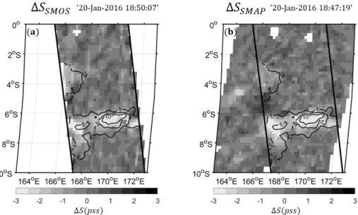
Figure 3 shows an example of a freshening event taking place during January 2016 in the SPCZ. During this event, SMOS and SMAP fly over the area of interest at less than 5-mn apart. IMERG RR colocated with SMOS SSS in a 15-min radius suggests there was a large RR event in this area, with a spatial pattern very close to the spatial pattern of SMOS and SMAP ΔS.
Figure 3: Study case, 20 January 2016, (a) SMOS salinity anomaly (b) SMAP salinity anomaly (black line are RR isolines in
b. Detection of rain history
Our goal is to distinguish the impact of the RR history on the observed SSS freshening from the impact of the instantaneous RR given the temporal auto-correlation of the RR (R??(δt)). Hence, we compare the observed temporal cross-correlation function between ∆S
and RR (ΓC+;??(δt)), with the one inferred from RR temporal auto-correlation function and
assuming that only instantaneous RR matters (ΓeC+;??(δt)) following equation (2) (r(X,Y)
correspond to the Pearson correlation between X and Y): RFF(GH) = I(JJ(H), JJ(H + GH))
ΓC4;FF(GH) = I(Δ)(H), JJ(H + GH))
ΓeC4;FF(GH) = ΓC4;FF(GH = 0) × JFF(GH) (2)
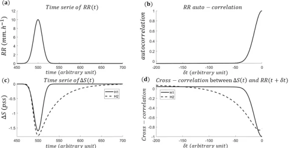
Figure 4 illustrates two idealized case studies respecting two different hypotheses. In the case of no-influence of RR history on ∆S (first hypothesis (H1)), ∆S depends only on instantaneous RR, ∆S (solid line on Figure 4c) then evolves in phase opposition with RR, the maximum cross-correlation is obtained with a time lag of 0 (Figure 4d, solid line). In the case of the influence of rain history (second hypothesis (H2)), some information on the rain event lasts after the rain abated, in other words, the salinity anomaly survives the rain event (Figure 4d dashed line). Then, the cross-correlation function is flattened towards negative time lags.
RR and ∆S time series are built as follows. For each pixel of the considered study area, we construct a one year time series of ∆S taken from SMOS and SMAP and a one year time series of RRP,-?. retaining data from SSMIS-F17, SSMIS-F16 and AMSR-2. Then we group
all pixel measurements per class of temporal shift (1-hour long) and compute auto-correlation and cross-correlation functions. We only retain cases with correlations computed with a minimum number of points of 1000 and a null hypothesis (no relationship between the two considered variables) rejected with a risk of error lower than 1%.
c. Filtering of non-rainy processes & ∆) versus instantaneous RR relationship
Figure 4: (a) Idealized Rain event (b) Auto-correlation function of RR for idealized rain event (c) Idealized salinity freshening due to the idealized rain event without influence of rain history (line) and with hypothetical influence of rain history (dashed-line). (d) Cross correlation function between RR and salinity freshening without (line) and with (dashed line) influence of time history. In b) and d) negative time lags concern rain before ∆S.
In order to study ∆S versus instantaneous RR relationship, SMOS, SMAP and SSMIS17 measurements are colocated within a 30-mn radius. However, before studying ∆S+,-+, ∆S+,./
and RR coherency, we start by filtering areas where temporal and spatial variability of ∆S are not due to rain. Our filtering methodology considers that rain events are very intermittent, leading to smaller monthly averaged absolute values of ∆S than ∆S associated with other processes that vary more slowly. We compute monthly running mean (∆S 2222) and standard deviation (σ+) of SSS in each pixel and day. Areas where ∆S variability is not dominated by
rain as river plumes or eddies have high absolute values of ∆S 2222. We empirically set a threshold value for ∆S 2222 and σ+: each pixel with ∆S 2222 lower than -0.65pss and σ+ higher than 1.75pss is
excluded from the study. Areas impacted by the filtering are shown on Figure 2, which particularly highlights river plumes. Some eddies with low monthly-averaged ∆S magnitude and edges of rivers plumes may be omitted by this filtering methodology, which will be a small source of error in computing the relationship between ∆) and RR. 0.5% of SMOS/SMAP/SSMIS17 collocated grid points are filtered by using this criterium.
To analyze filtering effects, we compare the relationships between ∆S and RR without and with filtering. Observed ∆S +,-+ versus RRP,-?. and ∆S +,./ versus RRP,-?. follow
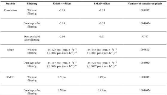
an almost near-linear relationship (Figure 5a and 5b). Data excluded by the filtering do not show any correlation between ∆S and RR contrary to not-filtered data (Table 2). Very low differences are found on correlation values when considering cases with and without filtering, but the RMSD of ∆S versus RR relationship decreases from 0.57pss to 0.54pss for SMOS and from 0.44pss to 0.40pss for SMAP when filtering is applied. The filtering does not significantly influence the slope of the relationship between ∆S and RR. Differences in correlation and RMSD between SMOS and SMAP datasets (Table 2) are consistent with the difference in their resolution.
For individual study areas, filtering does not influence the correlation level except in the Gulf of Mexico area. The filtering helps to remove large anomalies related to the river plume of Mississippi River and improves the correlation from -0.15 to -0.19 (-0.37 to -0.43 when taking only rainy cases into account).
Table 2: Statistics at global scale of ∆) versus JJSTUFV relationship for different filtering (Slope is obtained with a linear
regression (W = ∆), X = JJSTUFV) and Root Mean Squared Error JY)Z = [(∆) − ∆)2222222222222222) = [(∆) − 0.16 JJ<)\ 222222222222222222222222222222 STUFV)\
with ∆)< estimated considering a relationship between ∆) and JJSTUFV).
Statistic Filtering SMOS <=50km SMAP~60km Number of considered pixels
Correlation Without filtering
-0.18 -0.23 10098821
Data kept after filtering -0.18 -0.25 10048024 Data excluded after filtering -0.04 0.01 50797 Slope Without filtering -0.1625 pss. (mm. h %&)%& ±0.0002 pss. (mm. h%&)%& -0.1645 pss. (mm. h %&)%& ±0.0001 pss. (mm. h%&)%& 10098821
Data kept after
filtering -0.1607 pss. (mm. h %&)%& ±0.0004 pss. (mm. h%&)%& -0.1626 pss. (mm. h %&)%& ±0.0007 pss. (mm. h%&)%& 10048024 RMSD Without filtering 0.61pss 0.49pss 10098821
Data kept after filtering
1.1.3 Results
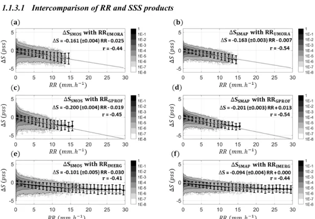
1.1.3.1 Intercomparison of RR and SSS products
Considering the three RR products, the ∆S+,-+ and ∆S+,./ follow nearly the same
dependencies with respect to RRP,-?. and RRa/?-b. Linear regressions are computed for the
three RR products but only UMORA and GPROF follow linear relationship with ∆S contrary to IMERG as shown on Figure 5. Slopes obtained with the linear regression are dependent of the RR product used but the Pearson correlation values (r) are the same for UMORA and GPROF. r values are lower with IMERG due to the non-linearity of the relationship with this RR product. The absolute value of ∆S versus RR slope obtained with GPROF is significantly higher than with UMORA. These differences of slope can be explained by the difference of RR distribution between UMORA and GPROF shown in Figure 1.
Figure 5 also illustrates similar values of ∆S standard deviations per class of RR between the different RR products. These values are however lower for ∆S+,./ in comparison with
∆S+,-+. Actually, the noise on ∆S+,./ is less than the noise on ∆S+,-+ in almost the same
ratio as the spatial integration of both instruments (50km or less for SMOS, ~60km for SMAP). The difference in resolution also explains lower values of r with ∆S+,-+ in comparison with
∆S+,./.
Figure 5: Relationship between ∆) and JJ (a) for SMOS and JJSTUFV (b) for SMAP and JJSTUFV (c) for SMOS and JJcdFUe
(d) for SMAP and JJcdFUe (e) for SMOS and JJfTgFc (f) for SMAP and JJfTgFc after filtering (black points are average per
class of RR and error bar standard deviation per class of RR. Grey lines are linear regression fit. The color scale corresponds to
the log10 of the number of occurrences). Pearson correlation coefficient are computed for RR higher than 1 mm.h-1 because RR
distribution between UMORA, GPROF and IMERG between 0 and 100. ℎ%& strongly differ due to the difficulty of identifying very
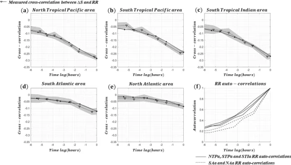
1.1.3.2 Which is the imprint of rain history on salinity anomalies?
For this particular study, we do not apply the filtering methodology in order not to remove a part of its possible signature. For this reason the rain history effect is not studied in the GMa area because of the influence of the Mississippi river plume. IMERG is not used here because of non-linearity between RR and ∆S (shown in section 1.1.3.1) and also in order to avoid the use of interpolated measurements.
Figure 6 (a, b, c, d, e) shows that very similar results are obtained in the different study regions. The maximum of ∆S/RR cross-correlation is recorded for the shortest time lag. NTPa area, STPa area and STIa show higher correlation levels compared to other areas because of a higher signal to noise ratio (larger RR in tropical regions and lower noise in satellite SSS in warm waters), and the NAa and SAa areas, which contain the less precise SSS, present the lowest correlation.
Figure 6 (a-e) and low error on the observed ∆S versus RR cross-correlation demonstrates that ∆S versus RR cross-correlation derived from RR auto-correlation fits very
well with observed ∆S versus RR cross-correlation in all areas. Only cross-correlations considering RR between 1 and 2 hours before ∆S measurements seem to show a correlation sligthly higher (in absolute value) in comparison with the estimated cross-correlation for NTPa and STPa areas. The differences in RR auto-correlation (Figure 6f) do not influence the correspondance between the observed ∆S versus RR correlation and ∆S versus RR cross-correlation derived from RR auto-cross-correlation. This result shows that the cross-correlation between ∆S and past RR is mainly due to the temporal auto-correlation of RR. Similar results are obtained by using RRa/?-b.
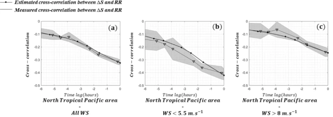
These results do not take into account the potential influence of WS. Figure 7 shows the computation of ∆S/RR cross-correlation for different classes of SMAP WS in the case of the
Figure 6: For each study area (a, b, c, d, e): (triangle) Temporal cross-correlation between ∆S and RR (individual triangles are linked with a dashed line) (dots) Estimated cross-correlation between ∆S and RR inferred from RR auto-correlation and correlation
between ∆S and instantaneous RR (individual dots are linked with a line). Grey colored areas show the 23 confidence interval for
the ∆S versus RR cross-correlation. Negative time lags concern rain before considered freshening. (f) RR auto-correlations for study areas.
NTPa area (chosen as one of the areas with the largest WS range (with SIa) and lower WS under rain). The classes of WS are defined as low WS (lower than the 0.3 quantile) and high WS (higher than the 0.7 quantile). If the low WS conditions are encountered over all the NTPa area,
high WS conditions are encountered closer to the equator. For salinity, only SMAP measurements are considered and we use SMAP WS. These results clearly show higher correlation between RR and ∆S for lower WS. In addition, despite larger uncertainties, the case with low WS presents higher ∆S/RR cross-correlation than expected considering only RR auto-correlation. This result seems to indicate an influence of rain history for temporal scales less than 5 hours in low WS conditions. This part of the study is limited by WS being only known at the time of the SMAP SSS measurement. WS influence on the relationship between RR and SSS freshening is developed in the next section.
Figure 7: For NTPa study area and SMAP: (a) all WS (b) WS under 5.5 0. h%& (c) WS above 8 0. h%&. For the three plots: (triangle)
Temporal correlation between ∆S and RR (individual triangles are linked with a dashed line) (dots) Estimated cross-correlation between ∆S and RR inferred from RR auto-cross-correlation and cross-correlation between ∆S and instantaneous RR (individual
dots are linked with a line). Grey colored areas show the 23 confidence interval for the ∆S versus RR cross-correlation. Negative
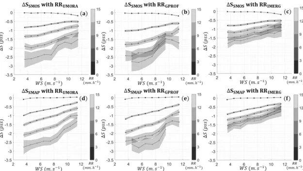
1.1.3.3 Variability of the relationship between salinity freshening and rain rate as function of wind speed.
We then investigate the WS dependency of ∆) as a function RR over the global ocean, using the filtering methodology (section 1.1.2.3c) and SMOS, SMAP as well as the three RR products. The results present a strong dependency of freshening for a given RR according to WS (Figure 8). In no-rain and low rain cases, ∆S+,-+ and ∆S+,./ show some biases for high
WS: a slight positive bias for ∆S+,./ and a slight negative bias for ∆S+,-+. Despite these slight
biases, SMOS (Figure 8 a, b and c) and SMAP (Figure 8 d, e and f) show very similar patterns. with the three RR products concerning the dependency with WS. Nevertheless, as observed in section 1.1.3.1, the magnitude of freshening differs strongly between RR products for each RR classes. RRa/?-b gives the more different relationship in comparison with RRP,-?. and
RRi,j?a. The latter RR show very similar magnitudes between 0 and 9mm. h%&, but over
9mm. h%& freshening measured for a given RR
i,j?a are lower than for the same RRP,-?.
value. Figure 8 also shows that significant freshenings are always observed even for high WS (between 10 and 12m. s%&).
Drushka et al. (2016) present a relationship allowing to express maximum ∆S (∆Sklm)
as a function of maximum RR (RRklm) and WS during a freshening event (3):
∆Sklm = a . RRklm . WS%p (3)
with a = 0.11 pss. (mm. h%&)%& and b = 1.1. Considering the SMOS and SMAP
estimates, we show that the rain history produces a negligible effect on freshening at satellite pixel scale. However, the influence of WS is important when considering instantaneous RR.
For this reason, we assume that ∆S and RR derived from satellites reflect in-situ ∆Sklm and
RRklm. Hence, we replace in this equation ∆Sklm and RRklm with ∆S and RR and derive
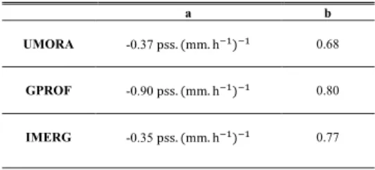
parameters a and b with RR and WS from satellite data. We found different a and b values according to the RR product used (see Table 3). Values of a and b computed with satellites ∆S
Figure 8: Relationship between ∆) and WSSMAP per class of RR: (a) with ∆)4TU4 and JJSTUFV (b) with ∆)4TU4 and JJcdFUe (c)
with ∆)4TU4 and JJfTgFc (d) with ∆)4TVd and JJSTUFV (e) with ∆)4TVd and JJcdFUe (f) with ∆)4TVd and JJfTgFc. Points
and RR are different from one RR product to another and very different from values obtained by Drushka et al. (2016).
Table 3: a and b coefficient for equation (2) considering JJSTUFV, JJcdFUe and JJfTgFc. Change of sign compared to
Drushka et al. (2016) is due to the fact that ∆)qrs is defined as the absolute value of the largest-in-magnitude negative value
of ∆) in Drushka et al. (2016).
a b
UMORA -0.37 pss. (mm. h%&)%& 0.68
GPROF -0.90 pss. (mm. h%&)%& 0.80
IMERG -0.35 pss. (mm. h%&)%& 0.77
1.1.4 Discussion & Conclusion
We have developed a filtering methodology that highlight ∆)+,-+ and ∆)+,./ only
where freshening is dominated by rain. ∆)+,-+ and ∆)+,./ are very consistent. They are
combined with RR retrieved from several satellites with different equator crossing times thus in order to investigate rain history imprint on SMOS and SMAP ∆S in various regions. For each of these regions, the apparent correlation between ∆S and past RR intensity is primarily explained by RR auto-correlation while ∆S magnitude is dominated by the instantaneous RR magnitude. Most commonly, the rain history influence seems to be negligible, even though a weak influence of rain history on ∆)+,-+ and ∆)+,./ is suggested at low WS (<5.5m s-1) for
durations up to 5 hours despite larger uncertainties. These results are consistent with model results obtained by Bellenger et al. (2017) showing that rain induced fresh lenses have short durations under moderate and high WS. Results obtained in this study show that WS mainly affects the relationship between instantaneous RR and freshening and seems to slightly influence the effect of rain history based on satellite estimations. Nevertheless, this result has to be taken with caution as it has been obtained considering WS+,./. L-band radiometers have
been shown to detect high WS under rainfall very well (Reul et al. 2016; Meissner et al. 2017) but the validity of moderate WS retrieved together with SSS under rain events has not been fully assessed. It is due to the difficulty of monitoring the wind speed integrated over ~50km resolution under rainfall by other means. The WS retrieval also depends on the quality of the prior WS (NCEP GFS in case of SMAP with a 1.5 m.s-1 error). Hence, further validation would
be necessary to fully assess the meaningfulness of our observation. In our analysis, we have confronted SMOS SSS with WS+,./ in order to minimise error correlations between SMAP
SSS and WS. Nevertheless, we cannot exclude that rain-induced roughness affects WS+,./ for
WS considered in this study (Tang et al. 2015) even if these effects can be moderated by the fact that they are important only at very low wind speeds and are negligible for moderate to high rain rates (we consider only WS higher than 3m s-1 in this study).
We provide a comparison of RRP,-?., RRa/?-b and RRi,j?a products, through ∆S
versus RR relationship. We find that despite different slopes in the relationship, UMORA and GPROF record similar correlation levels with ∆S (Table 3). This same level of correlation indicates that SMOS and SMAP freshenings are not able to distinguish RRP,-?. and RRa/?-b
pattern globally. The difference of slope is due to the difference of RR distribution between UMORA and GPROF (Figure 1). RRP,-?. are higher than RRa/?-b from 2 to 15 mm. h%&
approximatively but higher RR are observed with RRa/?-b. RRi,j?a shows a very close to
RRP,-?. behavior for the RR versus ∆S relationship (equation 3) but RRi,j?a records higher
RR than RRP,-?. which saturates at high RR (Figure 1). Additionnaly, RRi,j?a and
(not shown). This proximity between RRi,j?a and RRP,-?. may be explained by the more
thorough calibrations performed in these products. For UMORA, radiometers are intercalibrated at the brightness temperature level. For IMERG, RR are calibrated with respect to the GPM Combined Radar-Radiometer (CORRA; Grecu et al. 2016) product that uses RR from GPM Microwave Imager (GMI) and Dual-Precipitation Radar (DPR) instruments (Huffman et al. 2018). IMERG RR values are also calibrated using GPCP data thereby modifying RR distribution. Use of the DPR with a finer resolution compared with microwave imagers may explain higher RR observed with IMERG relative to UMORA.
We show that for the range of WS between 3m. s%& and 12m. s%&, ∆S versus RR
relationship is modulated by WS, leading to different relationships in the different areas. These results are in line with results obtained by Meissner et al. (2014). However, the methodology that we use in this study to compute ∆S allows us to homogenize the ∆S versus RR relationship over all oceans for a given WS. As described in previous studies (e.g. Boutin et al. 2016), the use of the Schlussel relationship describes at first order the ∆S versus RR relationship observed with satellites. However, the Schlussel relationship take into account only the molecular diffusion layer for salinity (0.05mm) but L-band satellite are influenced by rain induced freshening at 1cm depth. These phenomena are considered by Drushka et al. (2016) and Bellenger et al. (2017) that use RR and WS to explain ∆S spatial and temporal variability. We consider in this study ∆Sklm and RRklm as equal ∆S and RR to retrieve ∆S, RR and WS
relationship determined in previous studies using satellite estimations. Derived coefficients differ from the Drushka et al. (2016) estimate. Diagnostic of these differences is a difficult, yet unsolved challenge. Dong et al. (2017) compared in-situ measurements with Drushka et al. (2016) coefficients for equation (3) and also found different coefficients corresponding to larger freshening for a given RR (using satellite RR) in comparison with freshening values found by Drushka et al. (2016). Differences of ∆),WS,RR relationships obtained in previous studies reveal the difficulties to compare results obtained at different spatial and temporal scales and for different depths and thus, the difficulties to compare in-situ measurements, model results and satellite estimations.
Scale influence on ∆),WS,RR relationships raise the question of heterogeneity effects. Rain history influence on freshening observed with in-situ measurements is not observed with satellite measurements. This may induce that part of the rain history effect is contained in an influence of WS considering instantaneous RR. These hypotheses need to be investigated in future studies. Understanding the influence of heterogeneity and its role on ∆);WS;RR relationship is needed to be able to isolate other phenomenon such as rain splashing.
This study provides a methodology that allows for the removal of the rainfall imprint from each SMOS or SMAP SSS estimation by using instantaneous RR from IMERG provided each 30-mn, proposing an alternative solution to RIM model that uses RR history from the past 24 hours.
There is a need to conduct detailed process studies to better understand the reasons for the differences between models and in situ measurements. It may lead to estimate distribution of global RR over oceans only considering ∆) measured from SMOS and SMAP and thus to add an independant diagnostic tool of the bias error between different rain products that may reach relative values of 20% over the eastern Pacific Ocean (Adler et al. 2011).
Acknowledgements:
This work was funded by the ESA STSE SMOS+Rainfall project and by the CNES TOSCA SMOS-Ocean and CATDS projects. Alexandre Supply PhD grant is supported by Sorbonne Université.
UMORA rain rates are distributed by Remote Sensing Systems. GPROF and IMERG rain rates are distributed by the Precipitation Processing System at the NASA Goddard Space Flight Center.
References
Abe H, Ebuchi N, Ueno H, Ishiyama H, and Matsumura Y. 2018. Aquarius reveals eddy stirring after a heavy precipitation event in the subtropical North Pacific. J. Oceanogr. https://doi.org/10.1007/s10872-018-0482-0.
Adler R.F., Gu G, and Huffman GJ. 2012. Estimating Climatological Bias Errors for the Global Precipitation Climatology Project (GPCP). J. Appl. Meteor. Climatol., 51, 84–99, https://doi.org/10.1175/JAMC-D-11-052.1.
Asher WE, Jessup AT, Branch R, Clark D. 2014. Observations of rain-induced near-surface salinity anomalies. J. Geophys. Res. Oceans. 119: 5483–5500. https://doi.org/10.1002/2014JC009954.
Bellenger H, Drushka K, Asher W, Reverdin G, Katsumata M, Watanabe M. 2017. Extension of the prognostic model of sea surface temperature to rain-induced cool and fresh lenses. J. Geophys. Res. Oceans 121: https://doi .org/10.1002/2016JC012429.
Boutin J, Martin N, Reverdin G, Morisset S, Yin X, Centurioni L, Reul N. 2014. Sea surface salinity under rain cells: SMOS satellite and in situ drifters observations, J. Geophys. Res. Oceans, 119, 5533–5545, doi:10.1002/2014JC010070.
Boutin J, Reul N, Maes C, Reverdin G, Delcroix T, Gaillard F. 2015. Sea Surface Salinity from SMOS satellite mission: a synthesis of the main 2010-2015 oceanic results in France, IUGG 2011-2015 report, pp 100-103, http://www.iugg.org/members/nationalreports/CNFGG_RapQuad_UGGI_2015.pdf
Boutin J, Chao Y, Asher WE, Delcroix T, Drucker R, Drushka K, Kolodziejczyk N, Lee T, Reul N, Reverdin G, Schanze J, Soloviev A, Yu L, Anderson J, Brucker L, Dinnat E, Garcia AS, Jones WL, Maes C, Meissner T, Tang W, Vinogradova N, Ward B. 2016. Satellite and in situ salinity: understanding near- surface stratification and sub-footprint variability. Bull. Am. Meteorol. Soc. 97 (10). http://dx.doi.org/10.1175/BAMS-D-15-00032.1.
Boutin J, Vergely JL, Marchand S. 2017. SMOS SSS L3 Debias v2 Maps Generated by CATDS CEC LOCEAN. http://dx.doi.org/10.17882/52804.
Boutin J, Vergely JL, Marchand S, D'Amico F, Hasson A, Kolodziejczyk N, Reul N, Reverdin G, Vialard J. 2018. New SMOS Sea Surface Salinity with reduced systematic errors and improved variability. Remote Sensing of Environment, 214, 115-134. Publisher's official version: http://doi.org/10.1016/j.rse.2018.05.022, Open Access version: http://archimer.ifremer.fr/doc/00441/55254/
CATDS. 2017. CATDS-PDC L3OS 2Q - Debiased daily valid ocean salinity values product from SMOS satellite. CATDS (CNES, IFREMER, LOCEAN, ACRI).
http://dx.doi.org/10.12770/12dba510-cd71-4d4f-9fc1-9cc027d128b0
Drushka K, Asher WE, Ward B, and Walesby K. 2016. Understanding the formation and evolution of rain-formed fresh lenses at the ocean surface, J. Geophys. Res. Oceans, 121, 2673–2689, doi:10.1002/ 2015JC011527.
Dong S, Volkov D, Goni G, Lumpkin R, and Foltz GR. 2017. Near-surface salinity and temperature structure observed with dual-sensor drifters in the subtropical South Pacific, J. Geophys. Res. Oceans, 122, doi:10.1002/2017JC012894.
Fore A, Yueh S, Tang W, and Hayashi A. 2017. SMAP Salinity and Wind Speed Data User’s Guide version 4.0, Jet Propulsion Laboratory, California Institute of Technology.
Fournier S, Reager, JT, Lee T, Vazquez-Cuervo J, David CH, Gierach, MM. 2016. SMAP observes flooding from land to sea: the Texas event of 2015. Geophys. Res. Lett. 43, 10,338–10,346. http://dx.doi.org/10.1002/2016GL070821.
Fournier S, Vialard J, Lengaigne M, Lee T, Gierach MM, Chaitanya AVS. 2017. Modulation of the Ganges-Brahmaputra river plume by the Indian Ocean dipole and eddies inferred from satellite observations. J. Geophys. Res. Oceans 122, 9591–9604. http://dx.doi.org/10.1002/2017JC013333.
Fournier, S, Vandemark D, Gaultier L, Lee T, Jonsson B, Gierach MM. 2017. Interannual variation in offshore advection of Amazon-Orinoco plume waters: Observations, forcing mechanisms, and impacts. Journal of Geophysical Research: Oceans, 122. https://doi.org/10.1002/2017JC013103.
GPM Science Team. 2016. GPM SSMIS on F16 (GPROF) Radiometer Precipitation Profiling L2 1.5 hours 12 km V05, Greenbelt, MD, Goddard Earth Sciences Data and Information Services Center (GES DISC), Accessed [09/05/2018] 10.5067/GPM/SSMIS/F16/GPROF/2A/05
GPM Science Team. 2017a. GPM AMSR-2 on GCOM-W1 (GPROF) Climate-based Radiometer Precipitation Profiling L2A 1.5 hours 10 km V05, Greenbelt, MD, Goddard Earth Sciences Data and Information Services Center (GES DISC), Accessed [09/05/2018] 10.5067/GPM/AMSR2/GCOMW1/GPROFCLIM/2A/05
GPM Science Team. 2017b. GPM SSMIS on F17 (GPROF) Climate-based Radiometer Precipitation Profiling 1.5 hours 12 km V05, Greenbelt, MD, Goddard Earth Sciences Data and Information Services Center (GES DISC), Accessed [09/05/2018] 10.5067/GPM/SSMIS/F17/GPROFCLIM/2A/05
Grecu M, WS Olson. 2006. Bayesian Estimation of Precipitation from Satellite Passive Microwave Observations Using Combined Radar–Radiometer Retrievals. J. Appl. Meteor. Climatol., 45, 416–433, https://doi.org/10.1175/JAM2360.1
Hasson A, Puy M, Boutin J, Guilyardi E, Morrow R. 2018. Northward pathway across the tropical North Pacific Ocean revealed by surface salinity: How do El Nino anomalies reach Hawaii? Journal of Geophysical Research: Oceans, 123, 2697–2715. https://doi.org/10.1002/2017JC013423
Henocq C, Boutin J, Reverdin G, Petitcolin F, Arnault S, Lattes P. 2010. Vertical variability of near-surface salinity in the Tropics: consequences for L-band radiometer calibration and validation. J. Atmos. Oceanic Technol. 27: 192–209. https://doi.org/10.1175/2009JTECHO670.1.
Hilburn KA, Wentz FJ. 2008. Intercalibrated passive microwave rain prod- ucts from the unified microwave ocean retrieval algorithm (UMORA. J. Appl. Meteorol. Climatol. 47: 778–794. https://doi.org/10.1175/ 2007JAMC1635.1.
Ho DT, Asher WE, Schlosser P, Bliven L, Gordon E. 2000. On mechanisms of rain-induced air–water gas transfer. J. Geophys. Res. 105: 24045–24057. https://doi.org/10.1029/1999JC000280.
Hou AY, Kakar RK, Neeck S, Azarbarzin AA, Kummerow CD, Kojima M, Oki R, Nakamura K, Iguchi T. 2014. The global precipitation measurement (GPM) mission. Bull. Am. Meteorol. Soc. 95: 701–722. https://doi.org/10 .1175/BAMS-D-13-00164.1.
Huffman G. 2018. GPM IMERG Final Precipitation L3 Half Hourly 0.1 degree x 0.1 degree V05B, Greenbelt, MD, Goddard Earth Sciences Data and Information Services Center (GES DISC), Accessed [08/03/2018] 10.5067/GPM/IMERG/3B-HH/05
Joyce RJ, Janowiak JE, Arkin PA, Xie P. 2004. CMORPH: a method that produces global precipitation estimates from passive microwave and infrared data at 8 km, hourly resolution. J. Clim 5: 487–503. https:// doi.org/10.1175/1525-7541(2004)005,0487:CAMTPG.2.0.CO;2.
Kerr YH,Waldteufel P, Wigneron JP, Delwart S,Cabot F, Boutin J, Escorihuela MJ, Font J, Reul N, Gruhier C, Juglea SE, Drinkwater MR, Hahne A, Martin-Neira M, Mecklenburg S. 2010. The SMOS mission: New tool for monitoring key elements of the global water cycle. Proc. IEEE 98: 666–687. https://doi.org/10.1109/jproc.2010.2043032.
Kidd C, Huffman G. 2011. Global precipitation measurement. Meteorol. Appl. 18: 334–353. https://doi.org/10.1002/met.284.
Kummerow CD, Olson WS, Giglio L. 1996. A simplified scheme for obtaining precipitation and vertical hydrometeor profiles from passive microwave sensors. IEEE Trans. Geosci. Remote Sens. 34: 1213–1232.
Meissner T, Wentz F, Scott J, Hilburn K. 2014. Assessment of rain impact on the Aquarius salinity retrievals. Proc. Ocean Salinity Science Workshop, Exeter, United Kingdom, ESA. [Available online at www.smos-sos.org/presentations-ocean-salinity-science-workshop.]
Meissner T, Ricciardulli L, and Wentz FJ, 2017: Capability of the SMAP Mission to Measure Ocean Surface Winds in Storms. Bull. Amer. Meteor. Soc., 98, 1660–1677, https://doi.org/10.1175/BAMS-D-16-0052.1
Pei S, Shinoda T, Soloviev A, Lien RC. 2018. Upper ocean response to the atmospheric cold pools associated with the Madden‐Julian Oscillation. Geophysical Research Letters, 45, 5020–5029. https://doi.org/10.1029/2018GL077825
Piepmeier, JR, et al. 2017. SMAP L-band microwave radiometer: instrument design and first year on orbit. In: IEEE Transactions on Geoscience and Remote Sensing. vol. 55. pp. 1954–1966. http://dx.doi.org/10.1109/TGRS.2016.2631978. (no. 4).
Reul et al. 2014. Sea surface salinity observations from space with the SMOS satellite: a new means to monitor the marine branch of the water cycle. Surv. Geophys. 35 (3), 681–722.
Reul N, Chapron B, Zabolotskikh E, Donlon C, Quilfen Y, Guimbard S, Piolle JF. 2016. A revised L-band radio-brightness sensitivity to extreme winds under Tropical Cyclones: the five year SMOS-storm database, Remote Sensing of Environment, Volume 180, Pages 274-291, ISSN 0034-4257, https://doi.org/10.1016/j.rse.2016.03.011.
Santos-Garcia A, Jacob MM, Jones WL, Asher WE, Hejazin Y, Ebrahimi H, Rabolli M. 2014. Investigation of rain effects on Aquarius Sea Surface Salinity measurements. J. Geophys. Res. Oceans 119: 7605–7624. https://doi.org/10.1002/ 2014JC010137.
Santos-Garcia, A Jacob MM, Jones WL. 2016. SMOS Near-Surface Salinity Stratification Under Rainy Conditions. IEEE Journal of Selected Topics in Applied Earth Observations and Remote Sensing 9 : 2493-2499.
Schlussel P, Soloviev AV, Emery WJ. 1997. Cool and freshwater skin of the ocean during rainfall. Boundary-Layer Meteorol. 82: 437–472. https://doi .org/10.1023/A:1000225700380.
Soloviev A, Lukas R, Matsuura H. 2002. Sharp frontal interfaces in the near- surface layer of the tropical ocean. J. Mar. Syst. 37: 47–68. https://doi.org/ 10.1016/S0924-7963(02)00195-1.
Supply A, Boutin J, Vergely JL, Martin N, Hasson A, Reverdin G, Mallet C, Viltard N. 2017. Precipitation estimates from SMOS Sea Surface Salinity. QJRMS. http://dx.doi.org/10.1002/qj.3110.
Tang W, Fore A, Yueh S, Lee T, Hayashi A, Sanchez-Franks A, King B, Baranowski D, Martinez J. 2017. Validating SMAP SSS with in-situ measurements. Remote Sens. Environ. http://dx.doi.org/10.1016/j.rse.2017.08.021.
Vergely and Boutin (2017), SMOS OS level 3: the Algorithm Theoretical Basis Document (v300), 05/05/2017, available on http://www.catds.fr/content/download/78841/1005020/file/ATBD_L3OS_v3.0.pdf?version=3.
Walesby K, Vialard J, Minnett PJ, Callaghan AH, Ward B. 2015. Observations indicative of rain-induced double diffusion in the ocean surface boundary layer. Geophys. Res. Lett. 42: 3963–3972. https://doi.org/10.1002/ 2015GL063506.
Wentz, F.J., K.A. Hilburn, D.K. Smith. 2012. Remote Sensing Systems DMSP SSMIS Daily Environmental Suite on 0.25 deg grid, Version 7. Remote Sensing Systems, Santa Rosa, CA. Available online at www.remss.com/missions/ssmi. [Accessed 18/04/2018].
Wentz, F.J., T. Meissner, C. Gentemann, K.A. Hilburn, J. Scott, 2014: Remote Sensing Systems GCOM-W1 AMSR2 Daily Environmental Suite on 0.25 deg grid, Version V.8, [indicate subset if used]. Remote Sensing Systems, Santa Rosa, CA. Available online at www.remss.com/missions/amsr. [Accessed 18/04/2018]
Wijesekera HW, Paulson CA, Huyer A. 1999. The effect of rain- fall on the surface layer during a westerly wind burst
in the western equatorial Pacific. J. Phys. Oceanogr. 29: 612–632.
https://doi.org/10.1175/1520-0485(1999)029<0612:TEOROT>2.0.CO;2.
Yu, L. 2015. Sea-surface salinity fronts and associated salinity-minimum zones in the tropical ocean, J. Geophys. Res. Oceans, 120, 4205–4225, doi:10.1002/2015JC010790.
Zappa CJ, Ho DT, McGillis WR, Banner ML, Dacey JWH, Bliven LF, Ma B, Nystuen J. 2009. Rain-induced turbulence and air–sea gas transfer. J. Geophys. Res. 114: C07009. https://doi.org/10.1029/2008JC005008.
View publication stats View publication stats