Discovering Structure by Learning Sparse Graphs
The MIT Faculty has made this article openly available.
Please share
how this access benefits you. Your story matters.
Citation
Lake, Brendan and Joshua Tenenbaum."Discovering Structure by
Learning Sparse Graphs." Proceedings of the 32nd Annual Meeting
of the Cognitive Science Society CogSci 2010, Portland, Oregon,
United States, 11-14 August, 2010, Cognitive Science Society, Inc.,
2010. pp. 778-784.
As Published
http://toc.proceedings.com/09137webtoc.pdf
Publisher
Cognitive Science Society, Inc.
Version
Author's final manuscript
Citable link
http://hdl.handle.net/1721.1/112759
Terms of Use
Creative Commons Attribution-Noncommercial-Share Alike
Discovering Structure by Learning Sparse Graphs
Brenden M. Lake and Joshua B. Tenenbaum
Department of Brain and Cognitive SciencesMassachusetts Institute of Technology {brenden, jbt}@mit.edu
Abstract
Systems of concepts such as colors, animals, cities, and arti-facts are richly structured, and people discover the structure of these domains throughout a lifetime of experience. Dis-covering structure can be formalized as probabilistic inference about the organization of entities, and previous work has op-erationalized learning as selection amongst specific candidate hypotheses such as rings, trees, chains, grids, etc. defined by graph grammars (Kemp & Tenenbaum, 2008). While this model makes discrete choices from a limited set, humans ap-pear to entertain an unlimited range of hypotheses, many with-out an obvious grammatical description. In this paper, we approach structure discovery as optimization in a continuous space of all possible structures, while encouraging structures to be sparsely connected. When reasoning about animals and cities, the sparse model achieves performance equivalent to more structured approaches. We also explore a large domain of 1000 concepts with broad semantic coverage and no simple structure.
Keywords: structure discovery, semantic cognition, unsuper-vised learning, inductive reasoning, sparse representation
The act of learning is not just memorizing a list of facts; instead people seem to learn specific organizing structures for different classes of entities. The color circle captures the structure of pure-wavelength hues, a tree captures the biolog-ical structure of mammals, and a 2D space captures the geo-graphical structure of cities (Fig. 1a, 1c, 5a). How does the mind discover which type of structure fits which domain?
Discovering structure can be understood computationally as probabilistic inference about the organization of entities. Past work has tackled this problem by considering rings, trees, chains, grids, etc. as mutually exclusive hypotheses called structural forms (Kemp & Tenenbaum, 2008). Forms are defined by grammatical constraints on the connections between entities; for example the ring form constrains each color to have two neighbors (Fig. 1a). After considering all of the candidate forms, the structural forms model selects the best fitting form and instance of that form. This can be a pow-erful approach; the model selects a ring for colors, a tree for mammals, and a globe-like structure for world cities. These structures can then predict human inductive reasoning about novel properties of objects (Kemp & Tenenbaum, 2009).
Despite its power, the structural forms approach is not clearly appropriate when structures stray from the prede-fined forms, and such exceptions are common in real world domains. While the genetic similarity of animals is cap-tured by an evolutionary tree,1everyday reasoning about ani-mals draws on factors that span divergent branches, including
1Even this structure has exceptions; for example, Rivera and
Lake (2004) provide evidence that at the deepest levels “the tree of life is actually a ring of life” where genomes fused.
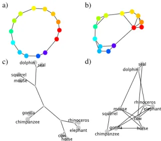
a) b)
c) d)
Figure 1: Structure learned by the structural forms model for colors (a) and mammals (c), compared to the sparse model (b, d). Shorter edges correspond to stronger connections. Graphs in this paper, except cities, were drawn with Cytoscape.
shared habitat, role as predator versus prey, and size. While these factors cannot be perfectly explained by a single tree, other domains are interestingly structured and are even fur-ther removed from a clean form, such as artifacts and social networks. Since humans learn and reason about all of these domains, they must entertain structural hypotheses without obvious grammatical descriptions.
These considerations have motivated models without an explicit representation of structure. Rogers and McClelland (2004) demonstrated how structure can emerge in a connec-tionist network mapping animals (like canary) and relations (can) to output attributes that a canary can do (grow, move, fly, and sing). Without being constrained to follow a tree, their network learns a distributed representation that approxi-mates a tree. But Kemp and Tenenbaum (2009) suggest some advantages of explicit representation: for incorporating ob-servations that have direct structural implications (“Indiana is next to Illinois”) and for learning higher-level knowledge (a tree helps learn the word “primate”, Fig 1c). It also remains to be seen if this model can predict human inductive infer-ences about animal properties, as past researchers have found this difficult (Kemp, Perfors, & Tenenbaum, 2004).
Here, we present an approach to structure discovery that in-corporates some of the best features of previous probabilistic and connectionist models. Rather than selecting between dis-crete structural hypotheses defined by grammars, the model
learns structure in an unrestricted space of all possible graphs. In order to achieve good inductive generalization, there must be a method for promoting simple graphs. While Kemp and Tenenbaum (2008) used grammars, here we use sparsity, meaning only a small number of edges are active. This struc-tural freedom can approximate cleaner strucstruc-tural forms, such as the ring-like graph for colors in Fig. 1b learned from simi-larity data printed in Shepard (1980), and on other datasets it deviates, such as mammals (Fig. 1d). Often these deviations capture additional information; while the tree suggests squir-rels and mice are equidistant from chimps, the sparse struc-ture suggests squirrels and chimps share additional similarity, like their association with trees.
The sparse model achieves performance equivalent to more structured approaches when predicting human inductive judgements. We show this for biological properties of ani-mals and geographical properties of cities (Kemp & Tenen-baum, 2009). Due to the model’s computational efficiency, it can learn on datasets too large for most previous approaches. We demonstrate learning a structure for 1000 concepts with broad semantic coverage, resembling classical proposals for semantic networks (Collins & Loftus, 1975).
The Sparse Model
In the structural forms and sparse models, a structure defines how objects covary with regard to their features. Objects are nodes in a weighted graph, where the strength of connectivity between two objects is related to the strength of covariation with regard to their features. The weights of the graph, de-noted as the symmetric matrix W , are learned from data by optimizing an objective function that trades off the fit to the data with the sparsity of the graph.
The data D is an n x m matrix with n objects and m features. The columns of D, denoted as features { f(1), ..., f(m)}, are assumed to be independent and identically distributed draws from p( f(k)|W ). If the graph structure fits the data well, fea-tures should vary smoothly across the graph. For example, if two objects i and j are connected by a large weight wi j
(like seal and dolphin), they often share similar property val-ues (“is active” or “lives in water”). As a result of sparsity, most objects are not directly connected in the learned graph (wi j= 0, like dolphin and chimp), meaning they are
condi-tionally independent when all the other objects are observed. Formally, the undirected graph W defines a Gaussian dis-tribution p( f(k)|W ), known as a Gaussian Markov Random Field (GMRF), where the n objects are the n-dimensions of the Gaussian. Learning GMRFs with sparse connectivity has a long history (Dempster, 1972), and recent work has formu-lated this as a convex optimization problem that can be solved very efficiently, in O(n3), for the globally optimal structure (e.g., Duchi, Gould, & Koller, 2008). Following Kemp and Tenenbaum (2008), we assume people learn a single set of parameters that fits the observed data well. Thus, we find the maximum a posteriori (MAP) estimate of the parameters argmax
W
log p(W |D) = argmax
W log p(W ) + ∑ m
i=1log p( f(i)|W ).
Generative model of features. Following the formula-tion in Zhu, Lafferty, and Ghahramani (2003), a particu-lar property vector f(k), observed for all n objects f(k)= ( f1(k), ..., fn(k)), is modeled as p( f(k)|W ) ∝ exp(−1 4
∑
i, jwi j( f (k) i − f (k) j ) 2− 1 2σ2f (k)Tf(k)).This defines a notion of feature smoothness, and it is equiva-lent to the n-dimensional Gaussian distribution
p( f(k)|W ) ∼ N(0, ˜∆−1),
where ˜∆ = Q −W + I/σ2is the precision (inverse covariance) matrix, Q = diag(qi) is a diagonal matrix with entries qi=
∑jwi j, and I is the identity matrix. We also restrict wi j≥ 0,
so the model represents only positive correlations. The model assumes the feature mean is zero, and raw data is scaled such that the mean value in D is zero and the maximum value in covariance m1DDT is one. The parameter σ2can be thought
of as the a priori feature variance (Zhu et al., 2003), and we choose the value that maximizes the objective function.
Sparsity penalty. To complete the model, we need a prior distribution on graph structures, p(W ). To learn a simple graph representation with a minimal number of edges, we assume each weight p(wi j) is independently drawn from a
distribution p(wi j) ∼ Exponential(β), meaning
p(W ) =
∏
1≤i< j≤n
βe−βwi j.
This prior encourages small weights, and in practice it pro-duces sparse graph structures by forcing most weights to zero.
Structure Learning. Finding argmax
W
log p(W |D) is equiv-alent to the following convex optimization problem:
maximize ˜ ∆ 0,W,σ2 log | ˜∆| − trace( ˜∆1 mDD T) −β m||W ||1 subject to ˜ ∆ = diag(
∑
j wi j) −W + I/σ2 wii= 0, i = 1, . . . , n wi j≥ 0, i = 1, . . . , n; j = 1, . . . , n σ2> 0.The first term in the objective, log | ˜∆| − trace( ˜∆m1DDT), is proportional to the log-likelihood from Kemp and Tenenbaum (2008) after dropping unnecessary constants, and mβ||W ||1,
where ||W ||1= ∑ni=1, j=1|wi j|, comes from the log-prior. ˜∆
0 denotes a symmetric positive definite matrix. The only free parameter, β, controls the tradeoff between the log-likelihood of the data and the sparsity penalty (||W ||1). A larger β
en-courages sparser graphs. As more features are observed (m increases), the likelihood is further emphasized in the trade-off. For all simulations, we set β = 14. The solution was found using CVX, a package for solving convex programs (Grant & Boyd, n.d.).
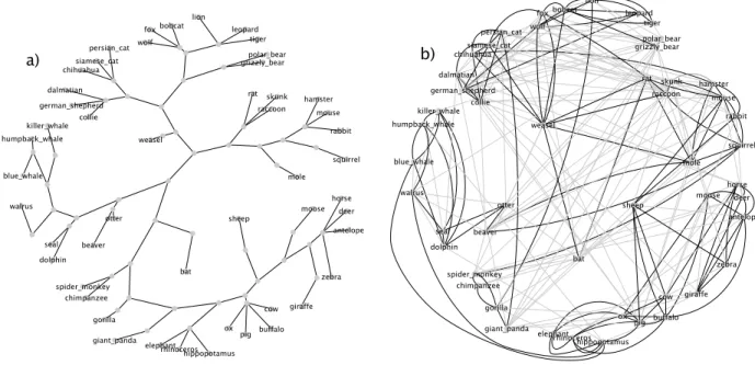
Figure 2: The (a) tree and (b) sparse graphs learned for mammals. Shorter edges in the tree correspond to stronger weights. The sparse graph is overlaid by node position, and thus edge length does not indicate strength. Strong edges w > .2 are in bold.
Taxonomic reasoning
Kemp and Tenenbaum (2009) learned a tree structure from a dataset of 50 mammals and 85 biological properties collected by Osherson, Stern, Wilkie, Stob, and Smith (1991). Prop-erties were various kinds of biological and anatomical fea-tures, including “is smart,” “is active,” and “lives in water,” and participants rated the strength of the association between each mammal and feature. The learned tree achieves high cor-relations when predicting human inductive judgments about novel biological properties. This predictive success may be due to the origin of these properties in the natural world; bio-logical relatedness is determined by an evolutionary process where species split and branch off. But there are reasons to suspect humans learn more complicated cognitive structures due to shared similarity across divergent branches, as dis-cussed in the introduction. Rather than constraining structure to be a tree, perhaps optimization with a sparsity constraint can learn appropriate structure for taxonomic reasoning.
Learning structure. Fig. 2 compares a tree learned by the structural forms model and a graph learned by the sparse model for the mammals dataset.2 The sparse model has 19% of possible edges active (w > .01), and stronger edges are highlighted in the figure. While the sparse model does not learn a tree, it captures some important aspects of the tree-based model. Major branches of the tree correspond to densely connected regions of the sparse model. The sparse graph captures some additional detail not represented by the
2The antelope had four missing color features which were filled
in from giraffe. They were left missing in the structural forms work. When learning any model from Kemp and Tenenbaum (2009), the best fitting σ2variance parameter was found, as in the sparse model.
In the original work this parameter was fixed at σ = 5.
tree. For instance, hippo is connected to the blue whale and walrus; although distant in the taxonomy, they are large and live in/around water. Similarly spider monkey and squirrel have a new link, perhaps due to agility and living in trees.
Property induction. A learned structure defines a prior distribution on properties of animals, which can be used for induction about new properties. Learning often involves gen-eralizing new properties to familiar animals; when a child first hears about the property “eats plankton,” the child makes decisions about which mammals this property extends to. To test the sparse and tree model, we apply them to two classic datasets of human inductive judgments collected by Osherson, Smith, Wilkie, Lopez, and Shafir (1990), which were also used in Kemp and Tenenbaum (2009). Judgments concerned 10 species: horse, cow, chimp, gorilla, mouse, squirrel, dolphin, seal, and rhino (Fig 1). Participants were shown arguments of the form “Cows and chimps require otin for hemoglobin synthesis. Therefore, horses require bi-otin for hemoglobin synthesis.” The Osherson horse set con-tains 36 two-premise arguments with the conclusion “horse,” and the mammals set contains 45 three-premise arguments with the conclusion “all mammals.” Participants ranked each set of arguments in increasing strength by sorting cards.
We compare the inductive strength of each argument for both the models and the participants (averaged rank across participants). Following Kemp and Tenenbaum (2009), to compute inductive strength in the models, we calculated the posterior probability that all categories in a set Y have the novel feature (in the above example Y = {horses})
p( fY = 1|lX) =
∑f: fY=1, fX=lXp( f )
∑f: fX=lX p( f )
A binary label vector lxis a partial specification of a full
bi-nary feature vector f that we want to infer. In the above ex-ample, X = {cows, chimps} and lX = [1, 1] indicating both
cows and chimps have biotin. Intuitively, Equation 1 states that the posterior probability p( fY= 1|lX) is equal to the
pro-portion of possible feature vectors consistent with lXthat also
set fY = 1, where each feature vector is weighted by a prior
probability p( f ) defined by the structure. We compute p( f ) by drawing 106feature samples from the Gaussian defined by that structure, converted to binary by thresholding at zero.
Performance of the sparse model is shown in column 1 of Fig. 3. The sparse model and tree-based model (column 2) perform equivalently and predict the participant data well. Both models outperform a spatial model (column 3, see Eq. 2) which embeds the animals in a 2D space, with particular advantage on the mammals dataset. The sparse, tree, and spa-tial models can be viewed as “cleaning up” the raw covariance matrix 851DDT, approximating it as closely as possible while satisfying certain constraints (sparsity, tree grammar, or 2D embedding). When compared to the raw covariance (column 4), the sparse and tree model show better performance.
r=0.91 Osherson horse r=0.91 Sparse Osherson mammals r=0.95 r=0.88 Tree r=0.84 r=0.73 Spatial r=0.81 r=0.8 Raw
Figure 3: Model performance on taxonomic reasoning. Hu-man ratings of argument strength (y-axis) are plotted against the model ratings (x-axis) for each argument.
Learning about new objects. In addition to learning about new properties, people constantly encounter new jects. How do the models learn about a new mammal, ob-served for just a few features? The tree-based model pro-vides strong grammatical guidance, but it might be difficult to make discrete placement decisions with only a few ob-served features. By contrast, the sparse model has no gram-matical guidance, so this provides an interesting comparison. Adding a new concept to the sparse model involves solving two convex programs. First, the model was trained on all but one mammal (49) and all properties (85). Second, the learned connections and variance were frozen, and the new concept was added while observing only a few features (10 or 20).3 Performance was evaluated on predictive ability for the missing properties (75 or 65). The models were tested
3Since many data entries are missing, simply skipping
miss-ing entries results in a covariance matrix that is not positive semi-definite. Instead we use a maximum likelihood estimate of the co-variance matrix found by Expectation-Maximization.
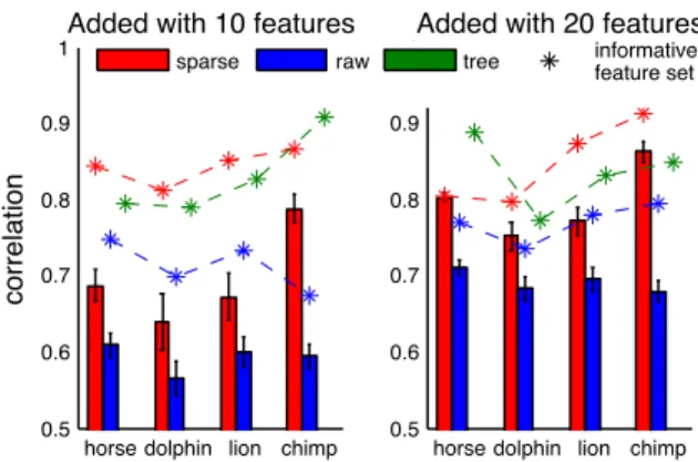
by adding four different mammals, where each addition was replicated 30 times with different random sets of observed properties. For each missing property, its expected value was calculated by performing inference in the Gaussian defined by the structure. Compared to the raw covariance matrix, the sparse model provided significantly better predictions of the missing features for each mammal tested (all 8 comparisons t(29), p < .01, Fig. 4). Since running all combinations is slow in the tree model, each model was also compared on an “informative feature set” ( *’s in Fig. 4), defined as the fea-ture set the raw covariance performed best on. For learning a new object with these features, the sparse model performs at least as well as the tree model.
horse dolphin lion chimp 0.5 0.6 0.7 0.8 0.9 1 correlation
Added with 10 features
horse dolphin lion chimp 0.5
0.6 0.7 0.8 0.9
1Added with 20 features
sparse raw tree informativefeature set
Figure 4: Each model adds a new object (seeing only 10 or 20 features), and the missing features are predicted. Bars are mean performance over 30 random feature picks, and stars (*) show performance from a single informative feature set.
Spatial reasoning
Geographical knowledge seems to require different structural representations than animals. Following the tradition of using Euclidean spaces to build semantic representations such as multidimensional scaling (Shepard, 1980), Kemp and Tenen-baum (2009) proposed learning a 2D space to represent the relationship between cities. This 2D space defines a Gaus-sian distribution with zero mean and covariance matrix K
Ki j=
1 2πexp(−
1
σ||yi− yj||2), (2) where yiis the location of the city i in 2D space. Kemp and
Tenenbaum (2009) found a double dissociation between the tree model and the spatial model, which only perform well on taxonomic and spatial reasoning respectively. Can the sparse model learn structures applicable to both domains?
Learning structure. Structures were learned from partici-pant drawings of nine cities on a piece of paper, and similarity was calculated from the pairwise distances (Kemp & Tenen-baum, 2009). This similarity matrix was treated as the raw covariance input to all the models. The learned spatial repre-sentation is compared to the learned sparse graph in Fig. 5. All the models require an assumed number of features, set to m= 85, preserving the β/m sparsity ratio from before.
Boston Denver Houston Orlando Minneapolis Durham San Diego San Francisco Seattle Boston Denver Houston Orlando Minneapolis Durham San Diego San Francisco Seattle a) b)
Figure 5: The (a) spatial and (b) sparse models learned from the city dataset. Graphs nodes are overlaid on the 2D space.
r=0.83 Minneapolis r=0.73 Houston r=0.76 Sparse All cities r=0.44 r=0.38 r=0.54 Tree r=0.8 r=0.75 r=0.83 Spatial r=0.89 r=0.81 r=0.86 Raw
Figure 6: Model performance on spatial reasoning. Human ratings of argument strength (y-axis) are plotted against the model rating (x-axis) for each argument.
Property induction. As in the taxonomic reasoning sec-tion, the models were compared to human data regarding property generalization. In an experiment by Kemp and Tenenbaum (2009), participants were presented a scenario where Native American artifacts can be found under most large cities, and some kinds of artifacts are found under just one city while other are under a handful of cities. An ex-ample inductive argument is: “Artifacts of type X are found under Seattle and Boston. Therefore, artifacts of type X are found under Minneapolis.” There were 28 two-premise argu-ments with Minneapolis as the conclusion, 28 with Houston as the conclusion, and 30 three-premise arguments with “all large American cities” as the conclusion. These arguments were ranked for strength, and mean rank was correlated with the model inductive predictions. The sparse model (column 1 of Fig. 6) provides good predictions, as does the 2D spa-tial model and the raw covariance matrix, which performs best (columns 3 and 4). The tree performs poorly (column 2). While there is a double dissociation between the tree and spatial model for taxonomic and spatial reasoning, the sparse model can predict human reasoning in both contexts.
Discovering structure for 1000 concepts
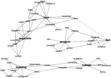
Learning sparse graphs can also be applied to domains with no simple structure. While animals may be fit by trees andFigure 7: Structure learned for 1000 concepts. This small subset shows the significant neighbors of the bold nodes (w > .2 except dotted edge w = .09). Shorter edges are stronger.
cities by 2D spaces, what type of structure organizes concepts as diverse as fruit, vegetable, fish, penguin, building, and col-lege? Human semantic reasoning operates in a huge semantic space, and here we learned a sparse model on an expansive domain of 1000 entities and 218 properties. A dataset of this size is prohibitive for the structural forms model as well as the connectionist model of Rogers and McClelland (2004).
Dataset and Algorithm. The dataset was collected by In-tel Labs (Palatucci, Pomerleau, Hinton, & Mitchell, 2009). Semantic features were questions such as “Is it manmade?” and “Can you hold it?” Answers were on a 5 point scale from definitely no to definitely yes, conducted on Amazon Mechanical Turk. To learn the optimal structure, we use a faster algorithm from Duchi et al. (2008) instead of a generic convex solver. For now, this requires two small changes to the model: wi jcan be positive or negative and a separate variance
term σ2i is fit to each object instead of one for all objects. Results. The structure learned from the entire data is very sparse with approximately 2.4% of edges active (|w| > .01). Fig. 7 shows snapshots of the network, consisting of nodes that are strong direct neighbors of either fruit, vegetable, fish, penguin, building, and college (w > .2). Fruit and vegetable are linked to subordinate examples, and connect to fish via a path through food. Interestingly, the network connects pen-guin to both sea animals (like fish and seal) and birds, high-lighting its role as an aquatic bird. Building and college are connected via several paths, including building–hotel– university–college and building–hotel–hospital–college.
To evaluate the sparse model’s predictive capacity for novel questions, we performed 4-fold cross validation, training on 3/4 of the properties and predicting the rest. The average test log-likelihood is −3.50 · 104 for the sparse model and −3.84 · 106for the raw covariance. The raw covariance
per-forms worse than in the past experiments since there are many more objects than features, and performance can be improved
by other regularization techniques such as Tikhonov (com-puted asm1DDT+vI for identity matrix I (Duchi et al., 2008)), which achieves a test log-likelihood of−3.63 · 104. Tikhonov
regularization does not significantly improve the raw covari-ance on the previous property induction tasks. Even though we fine-tuned the Tikhonov parameter v = .17 to the test sets, the sparse model still performs better with its parame-ter β = 14 fixed across all experiments in this paper.
General Discussion
Here we applied the sparse model to taxonomic and spatial reasoning. Past work has found a double dissociation be-tween these inductive contexts (Kemp & Tenenbaum, 2009), where a tree model and a spatial model provide good fits to only one context. However the sparse model is able to predict human inductive judgments in both contexts, by emphasiz-ing sparsity in structural representation. In addition to these inductive tasks, we applied the sparse model to a dataset of 1000 concepts with broad semantic coverage and no simple structure. The sparse model learned reasonable structure and outperforms simple regularization on novel features.
The sparse model also provides a probabilistic foundation for classic models of semantic memory such as semantic net-works (Collins & Loftus, 1975). Semantic netnet-works stipulate that concept nodes are connected to related concepts by vary-ing degrees of strength. These networks resemble the large structure learned for 1000 concepts (Fig. 7), suggesting the sparse model can be used to learn semantic networks from data. The sparse model is also related to Pathfinder networks (Schvaneveldt, Durso, & Dearholt, 1989) that find the mini-mal graph that maintains all pairwise sum-over-path distances between objects. While highlighting important structure, it retains the same similarity matrix from input to output, lack-ing the regularization that is important in our simulations.
While the sparse model is an important first step, it leaves out desirable features of previous connectionist and proba-bilistic models. The Rogers and McClelland (2004) model accounts for a rich array of phenomena from development and semantic dementia, yet to be explored with the sparse ap-proach. Compared to structural forms, the sparse model does not learn latent nodes (compare Fig. 1c,d), which increase sparsity and could be important for learning higher-level con-cepts such as “mammal” or “primate” (Kemp & Tenenbaum, 2009). Future work will use the sparse approach to explore learning deeper conceptual structure with latent variables.
Acknowledgements
We thank Intel Labs for providing their 1000 objects dataset, Charles Kemp for providing code and datasets for learn-ing structural forms, and Venkat Chandrasekaran, Ruslan Salakhutdinov, and Frank J¨akel for helpful discussions.
References
Collins, A. M., & Loftus, E. F. (1975). A spreading activation theory of semantic processing. Psychological Review, 82, 407-428.
Dempster, A. P. (1972). Covariance selection. Biometrics, 28, 157-175.
Duchi, J., Gould, S., & Koller, D. (2008). Projected subgradi-ent methods for learning sparse gaussians. In Proceedings of the twenty-fourth conference on uncertainty in AI (UAI). Grant, M., & Boyd, S. (n.d.). CVX: Matlab software for
disciplined convex programming. Retrieved 2009, from http://stanford.edu/∼boyd/cvx
Kemp, C., Perfors, A., & Tenenbaum, J. B. (2004). Learn-ing domain structures. In ProceedLearn-ings of the twenty-sixth annual conference of the cognitive science society. Kemp, C., & Tenenbaum, J. B. (2008). The discovery of
structural form. Proceedings of the National Academy of Sciences, 105(31), 10687-10692.
Kemp, C., & Tenenbaum, J. B. (2009). Structured statisti-cal models of inductive reasoning. Psychologistatisti-cal Review, 116(1), 20-58.
Osherson, D. N., Smith, E. E., Wilkie, O., Lopez, A., & Shafir, E. (1990). Category-based induction. Psychological Review, 97(2), 185-200.
Osherson, D. N., Stern, J., Wilkie, O., Stob, M., & Smith, E. E. (1991). Default probability. Cognitive Science, 15, 251-269.
Palatucci, M., Pomerleau, D., Hinton, G., & Mitchell, T. (2009). Zero-shot learning with semantic output codes. In Y. Bengio, D. Schuurmans, & J. Lafferty (Eds.), Advances in neural information processing systems (NIPS).
Rivera, M., & Lake, J. (2004). The ring of life provides evidence for a genome fusion origin of eukaryotes. Nature, 431, 152-155.
Rogers, T. T., & McClelland, J. L. (2004). Semantic cog-nition: A parallel distributed processing approach. Cam-bridge, MA: MIT Press.
Schvaneveldt, R. W., Durso, F. T., & Dearholt, D. W. (1989). Network structures in proximity data. In G. Bower (Ed.), The psychology of learning and motivation: Advances in research and theory(Vol. 24). Academic Press.
Shepard, R. N. (1980). Multidimensional scaling, tree-fitting, and clustering. Science, 210, 390-398.
Zhu, X., Lafferty, J., & Ghahramani, Z. (2003). Semi-supervised learning: From gaussian fields to gaussian pro-cesses(Tech. Rep. No. CMU-CS-03-175). Carnegie Mel-lon University.