en fr

HAL Id: hal-02577074

https://hal.inrae.fr/hal-02577074

HAL is a multi-disciplinary open access archive for the deposit and dissemination of sci-entific research documents, whether they are pub-lished or not. The documents may come from teaching and research institutions in France or abroad, or from public or private research centers.

L’archive ouverte pluridisciplinaire HAL, est destinée au dépôt et à la diffusion de documents scientifiques de niveau recherche, publiés ou non, émanant des établissements d’enseignement et de recherche français ou étrangers, des laboratoires publics ou privés.

Non holonomic local navigation by means of time and

speed dependent artificial potential fields

Nicolas Clavel, René Zapata, Francis Sevila

To cite this version:

Nicolas Clavel, René Zapata, Francis Sevila. Non holonomic local navigation by means of time and speed dependent artificial potential fields. 1st IFAC International Workshop on Intelli-gent Autonomous Vehicles, Apr 1993, Hampshire, United Kingdom. pp.235-240, �10.1016/S1474-6670(17)49305-0�. �hal-02577074�

NON-HOLONOMIC LOCAL NAVIGATION BY MEANS OF

TIME

AND

SPEED

DEPENDENT

ARTIFICIAL

POTENTIAL FIELDS.

N. CLAVEL*, R. ZAPATA**, F. SEVILA*.

*CEMAGREF. BP. 5095. 34080 Montpellier Cedex J. France **LIRM. Place E. Balaillon. 34000 Montpellier Cedex. France

Abstract : The study presented here concerns the local navigation problem of mobile robots, using the Artificial Potential Fields method. First, a solution 10 solve it main basic limitation, the local minima presence in the potential field, is proposed. This is done by a systematic local reshaping that allows 10 conserve the low complexity and the local aspect of the basic method. In a second time, a theoretical analysis of mobile robot non holonomic constraints leads to introduce a new concept : the "electrostatic like" or speed-dependent potential fields. Those repulsive fields create on the robot a continuous varying centrifugal force that realises the obstacles avoidance and respects non holonomy. Simulation results are very encouraging when we respect the basic assumption that the robot does not have to manOeU\Te.

Keywords: Local navigation, artificial potential fields, local minima, non-holonomy, Lagrange's multipliers, speed control.

l. INTRODUCTION

The navigation of a mobile robot needs two main complement ways : global and local methods. The former offers the opportunity of optimal trajectories (Brooks, 1983) and manoeuvring (pommier, 1991) but suppose the knowledge of the complete workspace. For this, integration of new obstacles or changing the goal during the mission is time consuming. On the other hand, the latter allows for unpre\iewed events but forbid any real optimisation. In this paper, we wiII address the particular local method based on the use of Artificial Potential Fields ("APF"). We will see that, replacing the repulsive APF by Artificial Electrostatic Like Potential Fields ("AELPF"), we are able to propose solution to the basic constraints of mobile robots : non-holonomy and continuity of the centrifugal force.

2. LOCAL MINIMA PROBLEM IN A.P.F

2. I Presentation.

First developed by Khatib (1975; 1985), the navigation algorithms using APF have interested many researchers because of their main advantages :

global or local aspect, low algorithmic complexity,

integration of robot inertial characteristics, natural understanding of the phenomenon and simple computation.

In fact, the navigation is realised by sol\'ing the following differential equation:

M(X).x" + Fe = -grad (Vg) (1)

M(X) ~ inertia matrix, X ~ configuration vector, Fc ~ centrifugal force,

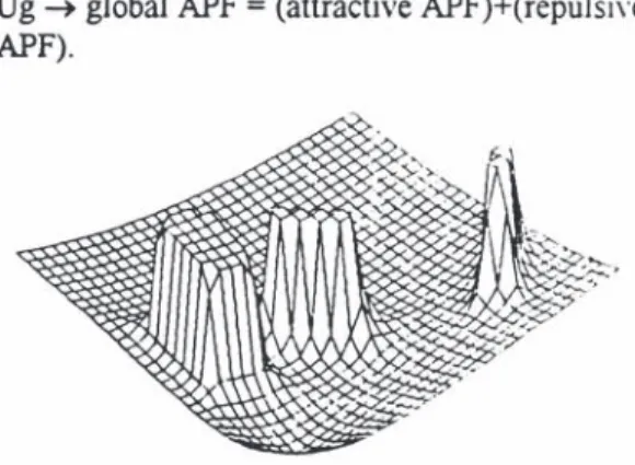
Ug ~ global APF = (attractive APF)+(repulsi\'e APF).

Fig. 1. Example of global APF

Consequently, the robot tends to fol1o\\ the maximum negative slope between its starting POilll and its target ("deep" value of the APF) a\'oiding obstacles (represented by peak values of the APF).

But, among some inherent limitations (Koren et al.,

1991), the major risk is the non-convergence induced

by the presence of local minima in the APF.

2.2 Some solutions.

Some solutions have already been proposed to solve

this problem. They can be separated into two classes

: those consisting of the construction of APF without

any local minimum (Khoditscheck, 1988; Megherbi

et 01, 1992; Nodorio 1989) and those which act when

the untimely convergence is done (Barraquand et ai,

1989; Latombe et aI, 1991).

The goal of this study is to find a solution as close by

the basic method as possible, conserving all its

advantages. The method proposed here, constitutes a

third class in the sense that it acts since the

movement starts. Applying it during the computation

of the all trajectory, there is no need to wait for the local convergence and path passing through saddles

can be found .

2.3 The solution systematic local deformation of

APF.

This solution has been developed by Clavel et al

(1992a; 1992b; 1993) and is based on the addition of

a new APF to the global one. Thus, the object is to

satisfy the two conditions : destabilisation and

ex1raction from the basin of attraction of the local

minimum. Let's see now what is the anal)tical mean

of this.

Destabilising a minimum. The natural way to

destabilise a local minimum is to transform it in a

local maximum. On account of studying the stability

of the robot, we use a Lyapunov function built with

the global APF as basis. For that, the Kinetic energy

of the robot is will be neglected : thus, the

destabilisation condition will be the strongest, independent of the state of the robot.

The study is made in the local domain that is the basin of attraction of the local minimum. It has been

shown (Clavel 1992b) that if the local APF

P(X) = F (X;Xmin) ... · .. (2)

is added to Ug" F being a continuous, positive,

finite, scalar decreasing function calculated with the origin in X min'

then, the destabilising condition on P(X) at the point

X_min is : slope (P) > -slope (Ug) ... (3) Ex1racting the robot from the local attracting

domain. After the destabilisation of the local

to the potential field [Ug(X)+P(X)] must follow

increasing values of Ug(X). This is translated in the

following condition on the Lie derivative:

the Lie derivative L of the potential function Ug(X) with respect to the vector field induced by Ug(X)+P(X) must be positive:

L [Ug(X)] Lgrad[Ug (X) + P(X)] > 0 ... (4)

This leads to (Clavel et al., 1992b; Clavel et aI,

1993) :

slope [P(X)] > -slope [Ug(X)]

1CI2 < Angle[grad(p(X),grad(Ug(X») < 31C12 ... (5)

Working up. The goal is to work up these two

constraints without studying each local basin of attraction (global aspect) or waiting for local

convergence. Consequently, the method is applied

since the movement starts and stopped just before the

goal. In fact, it means that the local destabilising

APF will be added systematically to the current point

of the trajectory.

It works as if the robot is always carrying his own

repulsive APF and we obtain a time varying global

APF:

Utotal (X,t) = Ug(X) + P(X,t) ... (6)

with the origin ofP(X,t) at the current point.

It can be sho\\n (Geenwood) that adding this time

dependent potential function doesn't change the conservativity of the system.

Experimental results. Figure 2 illustrates the

destabilisation action of the proposed method when

the robot meets local minima.

withoul the wave ... -Jo.: wave

r-~--~~--~~-." ~" --- --~ --1

~I

..

I

t

~----..:'---oo

~

~~=c~~~

~

.

..

,

~

1

~

~--

~

--~

,

i

",

-

---

minimum, the robot have to be pushed out of the Fig. 2. Examples of the local APF action

local basin of attraction D. To extract the robot from

2.4 Conclusion.

A method developed for mending the initial local navigation by use of APF have been presented. The results obtained appear to solve most of the basic limitations and allow to conserve the advantages. If few failure cases are observed (problem of periodic trajectories (Zhao, 1992) are not solved), the advances are very important.

3. NON HOLONOMIC CONSTRAINT AND APF Having resolved most of the local minima onfigurations of the APF, the study will now objects to the non-holonomic constraint of a mobile robot. Before discussing this point, first let examine the automatic meaning of the APF method.

3.1 Automatic approach of APF.

The automatic approach of the APF recalled now have been presented first by Khoditscheck (1988).

Force-control or a mechanical system in the state space. Suppose that the system is a point. Let define

S as the state space of the system. A point of S has for coordinates the vector p = (PI .P2)t with: PI = (x,y) and P2 = (x',y'). The Simplified Dynamical Principle. gives: P2' = M-I(p)*u ... (7) with u the control variable and M(P) the inertial matrix.

Force Control in the state space means that we are looking for p' = F(P,u) that is :

s' = F(P2) + ( 0 • M-I(p)*u)t ... (8) ~ F (P2) = ( P2 ,O)t...··· ... (9)

Closing the loop with the APF method. Now, let us see what the APF means in this automatic approach. The variable control u is now the force induced by the APF. So, the loop just have to be closed with u= -grad (Ug) (see fig. 5).

3.2 Classical approach of non-holonomy : Lagrange multipliers.

The problem of mechanical systems submitted to non-bolonomic constraints has been solved by Lagrange, using the method named " Lagrange's multipliers method". We will briefly present it and show wby it can not be used directly in the problem of navigation via APF.

Method of La gran ge's multipliers. Consider a system of n particles and the set of 3n Cartesian coordinates {Xi} associated. Suppose that each Cartesian coordinate lies with a set of n generalised coordinates {qj} via the 3njj differentiable functions:

Xi = fi (qI. q2,···.qn.t}··· (10) The m non-holonomic or holonomic constraints associated to the system are written as :

k(i=l.n) aji dqi + ajt·dt = 0 ... (11) withj: 1 •...• m; aji and ajt : functions ofthe q's and timet.

The idea is to associate a generalised force to each constraint, in order to make the generalised coordinates satisfied :

k(i=l.n) aji .oqi =0 ... (12) In fact, (12) means that the virtual displacement of each generalised coordinates satisfies the constraint associated. It can be shO\\n (D'Andrea-Noyel et al., 1992) that the constraint force Ci allo\\ing to respect this constraint on the motion is :

Ci = k(j=l,m) Aj.aji ... (13) \\ith Aj the Lagrange multiplier. .

Now. the Lagrange equation ofthe d)namic is :

dldt (oLloq'i) - (OLloqi) = k(j=l,m t.j aj,i ... (1.+) with L= (Kinetic energy)-(potential energy).

Application to the APF method. In the Cartesi:ln

space, Lagrange's dynamical equations can be written in the Euler-Ne\\10n formalism:

M(X).X" + }l(X.X') + g(X) = - grad [Ug(X)) .... (15)

u with X : configuration vector restricted to (x.),),

t-£--,...o-.r-+-}l(X,X') : Corriolis and Centrifugal forces, g(X)

L...-_ _ ---I

Fig. 5. Block scheme

gravity term.

In the case of a mobile robot g(X) = 0 and we neglect Corriolis's term. Thus }lCX.X') represents the centrifugal forces only.

Using (14) (15) (16), the system we have to solve

becomes (D'Andrea-Novel et al., 1992) :

M(X).X" + ~(X,X')= -grad [Ug(X)] + A.st(e)

S(e).x'=o

And we obtain:

1.= .ox. sine

+

with Qx = -Ux, Qy = -Uy,

-grad[Ug(X)] = (-Ux ; _Uy)t

Automatic interpretation. The constraint force Q adds to the system a force that will oblige the robot to respect the constraint. The block-scheme is now (see fig. 6.) :

Fig. 6.

Here appears the difficulty to use the Lagrange's

multipliers in the APF method. In effect, the

constraint force comes from a kinematic constraint and acts on the system as a "controller" on the applied ex1emal forces.

Now let us examine how the APF method acts. The

APF' are built to respect unilateral holonomic

constraints: the avoidance of the obstacles. For this,

the shape of the repulsive potential fields depends on

the geometry of the obstacles. If we modify its action

in order to respect Kinematic constraints, we induce

a conflict with the avoidance ones. The result is often

that the robot is locked on the boundary of the

obstacles. So, we have to find a force field depending

on both the Kinematic state of the robot and the

obstacles geometric criterion.

4. NON-HOLONOMIC AVOIDANCE VIA

ELECTROSTATIC LIKE POTENTIAL FIELD

In the following, x y have to be controlled and 8

bounded. We define X = (x, y) and q= (x, y, 8).

4.1 Non-holonomy and Electrostatic Potential Fields.

Greenwood (1988) has shown that if there exists a

potential field E which verifies the standard form of Lagrange's (18) then, the standard form of Lagrange's equation applies : the system is

conservative.

dldt (oE/oq'j) - (oE/oqi) = Qi i=I, ... n ... (IS)

Moreover, the system have to espect non-holonomic

constraints so that (14) is verified :

dldt (oUSq'i) - (oUSqi)

=

So, if a potential field E such that

dldt (oElSq'j) - (oElOqi) = Qi = L(i=I,m) Aj aj!i,. (19)

can be found, then, the system IS conservatIve and

the solution respect the non holonomic constraint.

4.2 Application to a mobile robot.

In the case of a mobile robot, A is the centrifugal

component of the sum of the applied forces (17).

As the centrifugal force is Fc = M(X).(ds/dt).(d8/dt),

we are looking for a potential field E which generates Q = Fc and verifies (IS).

4.3 Condition on the centrifugal force.

In a physical system, accelerations can not be

infinite. That means that the function d8/dt must be

continuous along the trajectory. This property will be

used to realise the obstacles avoidance. Let us define

h, a continuous function of X :

h (X) = d8/dt ...... (20)

As in the classical APF method, h is used to take into

account the position of the robot and the obstacles

characteristics. Thus, the potential field E will

respect the bilateral holonomic constraints

(avoidance) and the non-holonolllic constraint by IIse

of an induced continuous centrifugal force.

Notice that this constraint on the centrifugal force is "dynamically" much more restrictive than the

non-holonomic one.

4.4 The Electrostatic Like Potential Field.

As seen before, the notion of conseT\'ative systems

can be extended to the Electrostatic Like Potential

Fields (ELPF) if and only if it respects (18).

Greenwood (1988) sho\\n that the potential field can

be written:

E = L(i=I, ... ,n) Ai (~,t). q'i ... (21) then, it respects Lagrange's equatIon and the force

induced is:

Qi = A'j - L(k=l, ... ,n) (oAk/oqi)·q'k. ... 22)

Let us define the Ai's. The robot is controlled in the

cartesian space so q = X = (x, y). Taking

Ax = M(X).f(x).y and Ay = M(X).g(y).x with f a

continuous function of x only and g a contmuous

can be used to model complex obstacles. The data on Qx = M(X).[f(x) + g(y»).y'

Qy = -M(X).[f(x) + g(y»).x' .(23) the obstacles are their lengths Lo and their widths 1₀,

Thus, as Q = M.e'.v(§4.2), taking e'= (f(x)+ g(y» induces Q equal to the constraint force of non-holonomy.

It has been proved that the electrostatic potential field respects the Lagrange's equations and the non holonornic constraints of the mobile robot.

In the case of multi-obstacles :

8'= Lo(fo(x), 8o(y» with.o=nurnber of obstacles .(24) and, as in the classical APF case f and g are built so that the nearest obstacle acts much more than the others.

5. AVOIDANCE FUNCTIONS

5.1 Initial condition.

It has been demonstrated that the electrostatic like potential field E is able to make the robot having a centrifugal force that respect the non holonornic constraints.

Using the functions f and g, obstacles avoidance can be realised. So, an attractive force .just have to be computed using a classical attractive potential field (See fig. 7. for the new block scheme).

The only restrictive condition is at the beginning of the movement. In fact, if the attractive force is not collinear with the orientation of the robot, the starting trajectory "ill be non holonornic because the change of orientation is not induced by the electrostatic potential field. This means that 8' is not equal to fex)+g(y).

For that, at the beginning, the robot have to be oriented in order to have the attractive force collinear to it orientation (in direction only).

Fig. 7.

5.2 Implementation.

When computing f and g, the obstacles are modelled

f and g are infinite on the boundaries of the obstacles, and must include the robot geometry (lr). So, the computation is :

f = f ( Cld(x), lo.lr) and g= g ( C/d(y), Lo,lr) with: - d(x), the distance to the side 10,

d(y) the distance to the side Lo, - C, constant coefficient.

In Zone I of Fig. 8. (respectively Il) the robot needs onIy the function f (resp. g) to starts the avoidance :

it uses the data 10 (resp. Lo). It uses the second parameter onIy when it is already able to know it via sensor : on the transition line (at this point of the trajectory we must have f=g).

The direction of avoidance is the one that requires the smallest deviation.

ZONE 11 Lo j I , ZONE I

T .

-

---:

I

Fig. 8. Basic avoidance strategy

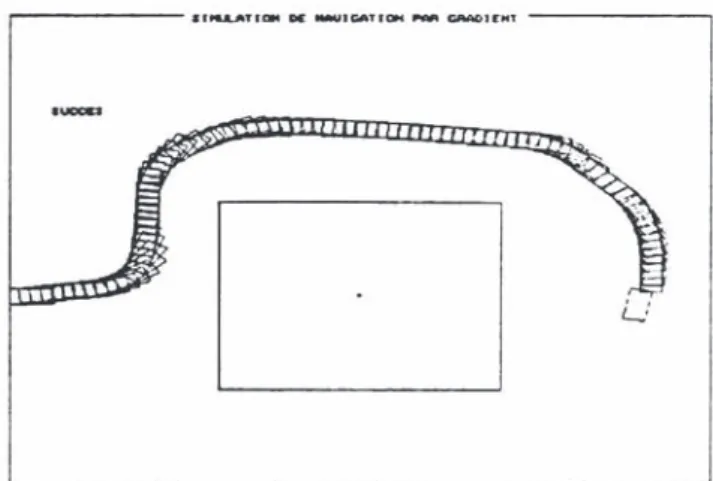
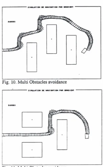
5.3 Simulation results.

As shown fig. 9.,10.,11. very good results on the shape of the trajectory have been obtained. The non holonornic constraint is always above zero (-10-17).

~----.'N.A..AT''* DC' ...,lGAT.~ ... GAAOll""' - - - ,

L.:'

by

qr

...

Fig. 10. Multi Obstacles avoidance

. - - - ' - - - - "MoLAl'" _ . . , . . . , . . . HIlII IIIIIIIIIDIENf - - - ,

...

D

D

Fig. 11. Multi Obstacles avoidance

5.4 Assumptions.

To realise this avoidance strategy, some assumptions have to be made :

- The robot does not have to manoeuvre.

- There is no obstacle in a circle centred on the goal and having a radius equal to robot length : at this step ofthe trajectory we realise a position control.

- Two near obstacles separate by less than robot

length are considered as one big obstacle.

6. CONCLUSION

First, a work on the local minima have been

presented. To solve this problem, a local APF have

been used extract the robot. This method will still be used in the ELPF method in order to be able to climb the attractive APF when the avoidance imposes it.

Compared to the APF method, two basic

characteristics of robot movement have been added

without gro~th of the complexity : non holonomy

and continuous centrifugal force. This last

characteristic makes this method useful even in the case of an arm movement.

The obstacle modelisation is based on rectangular shape which can be associate for complex obstacles

(we are working on this perception problem). Notice

that the data required at any step of the trajectory correspond to those the robot can "see".

It is expected that through a good choice of

avoidance functions in order to bound 8', and the

addition of a frictional force to bound v, leads to compute directly the speed control of the robot.

REFERENCES

d'Andrca-Novcl. B., Butin. G. Campion, G. (1992). Dynamic

feedback of non-holonomic wheeled mobile robots. IEEE

intemalional conference on robotics and au/omations, Mu (France), May 1992,2527-2532 .

Barraquand, 1 .• Latombe, I.C. (1989). On non-holonomic robots

and optimal manoeuvring. Revue d'inzelligence artificielle,

3(2), 1989.

Brooks, R. (1983). Solving the find path problem by good

representation of free space. I. E.E.E. , March-April .

Clavel, N., Zapata, R., S6vila, S. (1992a). Local navigation by

means of artificial potential fields : surfing on a time

dependent local de deformation. Au/omazione 1992, 36·

congru anuaJ of AMPLA,16-18 Nov. 1992.

Clavel, N .• Zapata, R., Sevila, F. (1992b). Local navigation by

means of time dependent potential fields : the wave

approach. IFTOM, Nagoya (Japan), September 1992.

Clavel, N., Thompson, P .• Sevila, F .• Zapata. R. (1993). A

mobile platform with a robotic arm working in a semi

structured environment. IFAC world congress. Sydney

(Aus/ralia) July 1993.

Greenwood. Principles of dynamics, £d. Prentice Hail

(New York), p. 290.

Khatib. O. (1978). Dynamic control of manipulations operating

in a complex environment. 3rd C.I.S.M. Udine (/Ialy),

12-15 September 1978.

Khatib, O. (1985). Real time obstacle avoidance for manipulators

and mobile robots. I.E.E.E. SI Louis (U.S.A.). 25-26

March 1985.

Khoditscheck. D.E. (1988). Robot navigation functions on

manifolds with boundary. Adv. in applied malh., July

1988.

Koren, Y., Borenstein, 1. (1991). Potential field methods and

their inherent limitations for mobile robot navigation. I.E.E.E Sacramenzo (U.S.A.), April 1991.

Latombe, J.C. (1991). Proceedings Joumees raisonnemenz

geombrique " de la perception vers /'action, llFlA [nstillll I.M.A.G., Grenoble 16-17 September 1991.

Megherbi, D .• Wolovitch. W.A. (1992). Real-time velo.;ity

feedback obstacle avoidance via complex variables and

conformal mapping. I.E.E.E. Mce (France). May 1992.

Nodorio, H. (1989). A potential approach for a mobile point

mobile robot on an impliciter potential field. I.E.E.E.

Tokyo (Japan). 1989.

Pommier , E.(1978). Generation de trajectoires pour robot

mobile non holonome par gestion des centres de rotation. PhD Thesis, L.I.R.M. Monrpeliier (France).

Zhao, Y .• BeMent, S.S.L (1992). Kinematics. dynamics and

control of wheeled mobile robots. IEEE inzemational

conference on robotics and au/omation, Mce (France), May 1992.91-96.