Differential Kolmogorov equations for transiting processes

(1)

Differential Kolmogorov Equations for Transiting Processes

by

Gael D6silles

Ingenieur Dipl6me de l'Ecole Polytechnique, France (1995)

Ing6nieur Dipl6m6 de l'Ecole Nationale Superieure de 1'Aeronautique et de l'Espace,

France (1997)

Submitted to the Department of Aeronautics and Astronautics

in partial fulfillment of the requirements for the degree of

Master of Science

at the

MASSACHUSETTS INSTITUTE OF TECHNOLOGY

June 1998

) Massachusetts Institute of Technology 1998. All rights reserved.

Author

.

...

Department of Aeronautics and Astronautics

April 1998

7/

Certified by ...

...

Eric Feron

Assistant Professor

Thesis Supervisor

Accepted

by...

...

..

Chairman, Department Committeb on Graduate Student

JUL

087~8

LIBRARIES

(2)

Differential Kolmogorov Equations for Transiting Processes

by

Gael D6silles

Submitted to the Department of Aeronautics and Astronautics on April 1998, in partial fulfillment of the

requirements for the degree of Master of Science

Abstract

This work develops a short theory on transiting stochastic processes, following standard guidelines in the theory of probabilities and stochastic processes. Transiting processes are processes submitted to It6's stochastic differential equations, with drift and diffusion depending on a Poisson random process. We establish the integro-differential equations satisfied by the probability density function of such a process, and also the one satisfied by the first passage conditional probability for a stopped

transiting process. As an application of this theoretical work, we show how existing probabilistic

models of aircraft behaviour in free flight, involving mainly Poisson and Gaussian processes but also other probability distributions, lead to quite simple differential equations for the probability density function of an independent aircraft, and for the probability of collision of two aircraft. The equations are solved numerically, using finite difference or finite element methods. We also propose other methods based on Fourier analysis.

Thesis Supervisor: Eric Feron Title: Assistant Professor

(3)

Acknowledgements

First of all, I am thankful to my advisor Eric Feron, who proposed me the exciting field of stochastic processes as applied to some security concerns in Aeronautics. As there was of course ups and downs in my work, he was keeping me on the right track, with a very supportive attitude. The lesson is, simplicity of ideas is always the trick.

I wish to thank Jaime Peraire, for he was the one who gave me this unforgettable opportunity to spend some time at MIT. My gratitude is the mirror of everything this year has brought to me.

I wish to sincerely thank Yashan Wang, my teacher in stochastic processes during Fall 1997. He made the technical and almost nowhere intuitive field of probability theory practical and intuitive, while mathematical rigor was always respected.

I wish to thank Alex Megretski, for the special spirit I tried to capture from his course during Spring 1997, not to mention the very deep discussions he is always ready to offer. His outlook on things was always to me the balance I needed to remain sighted.

I wish to thank the team of ICE Lab, and maybe especially Emilio Frazzoli, for their very nice welcome and the help they always provided when I needed it. I also thank them for not asking why I was never in the lab, but sometimes remotely...

(4)

List of Figures

1-1 Flow chart of Poisson transfers ... ... . 11

1-2 Example of application (1) ... ... 31

1-3 Example of application (2) ... . ... ... 31

1-4 Example of application (3) ... ... ... 32

1-5 Example of application (4) ... ... .. 32

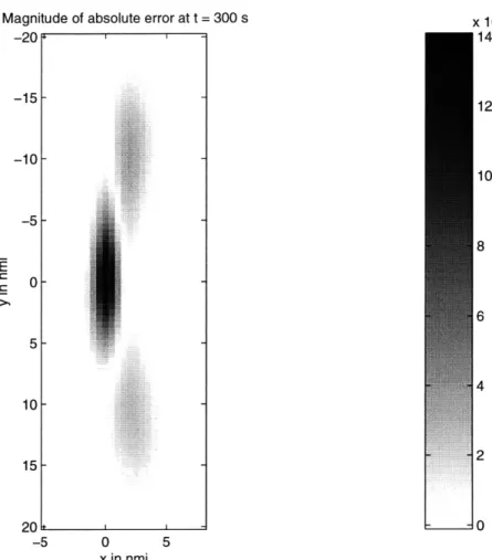
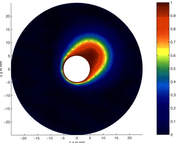
2-1 Probability density function of the intruder, in a case of numerical instability . . . . 42

2-2 Comparison between a coarse and a narrow grid . ... . 43

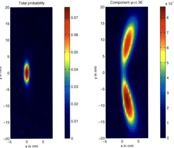
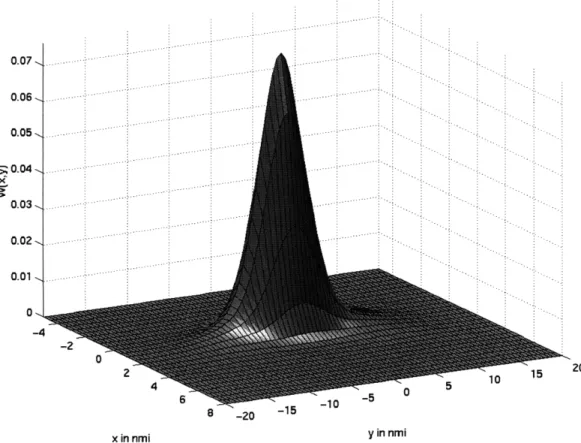
2-3 Probability density function of the intruder (1) ... .. 44

2-4 Probability density function of the intruder (2) ... .. 45

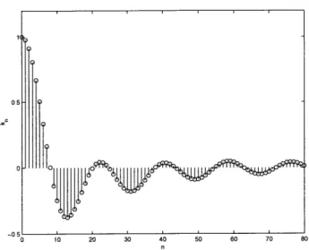
2-5 Fourier coefficients of k ... ... 48

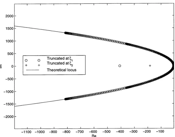
2-6 Eigenvalues in the Fourier method ... ... 49

(7)

Introduction

One future perspective in sight in the Air Traffic Management is to release the hard constraints of the flight, letting the pilots make their own decisions [6, 1, 17], with the help of automated and autonomous systems aboard. The main issue here is to design alert systems to assist pilots and controllers resolve conflicts between aircraft.

One way to address the design of such systems is to imitate the behaviours of the pilots by statistical models and deduce from them predictions, such as speed, altitude, heading, etc. Among the statistics of first concern, the probability density function of an isolated airplane has shown authorizing an analytical calculation, or at least a semi-analytical one. On that statistical back-ground, high safety standards require extreme accuracy in the computation of the probability. Two approaches have been proposed so far : one is to simplify the hypotheses of the problem, by modeling reality with Gaussian processes, on the purpose to achieve analytical solutions [1]; the other is to use Monte-Carlo simulation techniques to evaluate the probabillity by trajectory launches [17].

The analytical approach, though very efficient, does not take into account natural behaviours of the pilots, for instance taking unknown actions like quick turns or changes of altitude. These decisions are critical as a conflict arises. Continuing improvements of computation means allow to now consider the resolution of a more general model by well-known numerical techniques, similar to those used in Computational Fluid Dynamics (analogies between probability density functions and mass density of a fluid are profound). As computation power increases, the hope of solving the problem with high accuracy and efficiency becomes more and more concrete.

Poisson processes are very frequently used in the modeling of physical systems, for they provide a mathematical model of events with mean frequency of occurrence, and very few hypotheses are needed on a process to be of the Poisson type [16]. While arrival times of customers in a post office are often the academic example of such processes, Poisson processes can also model the decision times of pilots of an aircraft, in the context of aircraft behaviour modeling.

However, as soon as Poisson processes are involved in a random process, the Chapman-Kolmogorov differential equation satisfied by the probability density function of the problem can take a very awk-ward form, typically infinite in the number of terms, as shown in references [4]. Poisson processes are actually not the only processes to infere infinite Chapman-Kolmogorov differential equations.

(8)

Examples of such infinite differential equations show the catastrophic results of truncating Taylor's expansions at a large, but finite, rank. The solutions to the truncated equation may converge weakly to the solution of the exact equation, but the weak convergence is at the price of enormous oscil-lations of the approximated solution around the exact one, causing the approximated probability density function to take on negative values - among other problems.

There is therefore a need to avoiding such a global approach. Master equations, that transform the infinite expansion of the Chapman-Kolmogorov equations into an infinite-dimensional problem, are here shown to be a possible attack, as applied to a model of aircraft behaviour in free flight proposed earlier.

(9)

Chapter 1 Differential Kolmogorov equation

for transiting Markov processes

The idea of the theory developed in the following lines is to find the evolution of the probability density function of a system at position x(t) changing of dynamics at random times. The probability distribution of the instants of change is assumed (a decreasing) exponential, that is to say the random process of the times of change is a Poisson process. First we consider the case of a finite set of possible dynamics driving the modile between two consecutive instants of switch. Second we extend the formalism to the more general case of a continuous set of dynamics. Our point of view is fully probabilistic, in the sense that the dynamics itself is not assumed deterministic. Formally, we will identify the change of dynamics to a change of system, and with this convention, a change of system will be called a jump. The best mental representation of the behaviour of such a mobile (or, more technically, a stochastic process) is a moving body with a trajectory depending on a parameter (for instance : the heading, the speed, the curvature, any geometrical characteristics of the trajectory...), such that the parameter changes of value at "Poisson times". The mathematical background needed is exposed in the next section.

1.1 Position of the problem, Notations

Let us consider n systems E, ... , E,, with n a finite integer. We assume that each of them can be completely defined by a vector-valued Markov process x, (t) E Rd, thus driven by a stochastic differential equation. We assume to know for each EY the transition probability p' (x, t I y, s), defined as the probability that the state xj (t) is at the position x at the instant t, given that xj (s) = y

(with s < t) :

(10)

The process driving Ej is not assumed stationary. We admit that the transition probability pi (x, t I y, s)

can be developed with respect to the time delay t - s as :

p7 (x, tI y, s) = 6(X -y) + p~ ( Y; s) (t - s) + o(It - s) (1.1)

where the term pt(x 1y; s) may be formally identified to

pt (x I y; s) = lim (P (x, s + ds I y, s) - 6( - y))

ds-+O, ds>O ds

The expansion (1.1) can be held each time the system Ej has continuous sample paths. It is no evidence that pt(xy; s) and pi(x, t I y, s) should be functions of their arguments x and y. It even

simplifies a lot further analytical developments to suppose that they are distributions. Hence, we will use the formalism of bilinear brackets (., .) in the following. We assume all distributions to be tempered, in the sense given by Laurent Schwarz [2]. To find the expansion (1.1), one may prefer to expand the Fourier transform of p3 (x, t I y, s) (with respect to the space variable x) as a Taylor

series in t - s, and then invert the expansion from the Fourier domain. In some major references

[4], the Taylor expansion (1.1) is split into three separate statements, involving functions instead of distributions.

We now suppose that the system x(t) randomly jumps from one given subsystem Ei to another subsystem Ej with probability P{ E -+ Ej

}

= Aij(t) dt during dt (with Aij(t) > 0 at any instant

t. Between two consecutive jumps, x(t) is thus driven by a unique subsystem at any time. In

mathematical terms, we define :

Ai(t) = lim P{ x(t + dt) E EYj x(t) E Ei }

dt-+O dt

It is the Poisson hypothesis that allows the limit to exist. There is no requirement on the functions

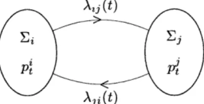
Ai, (t) to be symmetric in the indices i and j. See Figure 1-1 for a graphic representation of the

process, in terms of flows.

We want to find a partial differential equation satisfied by W(x, t), the probability density func-tion of the process x(t), or the probability to find x(t) at the posifunc-tion x and instant t :

W(x, t) = dP{x (t) = x}

(11)

Figure 1-1: Flow chart of Poisson transfers between subsystem i and subsystem j.

1.2 Practical treatment

1.2.1 Expansion of the conditional density functions

Let W (x, t) be the conditional probability density function defined by

WJ(x,t) = dP{x(t) = xIx(t) E Ed}

Using a Chapman-Kolmogorov equation, we may write

W3 (x, t + dt) = i 1 - E j ifAj i ( t ) d t (PJ (x' t + dt 1. t) , WJ(., t))

+ dt Aiji(t)(p(x , t + dt .,t), Wi(., t)) (1.2)

This relation can be easily understood if interpreted in terms of flows of particles; in that context indeed, WJ(x, t) may be seen as the fraction of the total number of particles in system Ej that are at position x at t. Between t and t + dt, some particles of Ek, with mass proportional to Wk(y, t) jump from any far y to the actual position x, and then get in E,, whatever k be (j itself or i : j). The first event occurs with probability pk (x, t + dt

I

y, t) by definition, whereas the second one has

probability Akj (t) dt.

Plugging the Taylor's expansion (1.1) for each pk (x, t + dt I ., t), and observing that by definition (6(X - .), Wk(., t)) = Wk(z, t), we get

W .(x,t + dt) = Wj (x,t) + dt [((xl .; t),t W ) ) - Ai(t) W (x, t)

+ A j (t) wV(x, t)I + (dt)

Hence, by letting dt tend to zero, W (x, t) must satisfy

8WJ

t (x, t) = (p(x ., t) , W(. ,t)) + , (A ,(t) Wi(x, t) - Aji(t) W (x,t)) (1.3)

(12)

1.2.2 Evolution of the masses

By a straight-forward conditional expansion, the probability density function we are searching for, namely W(x, t), reads :

W(x,t) = W(x, t) P{x(t) E E3}

where P{x(t) Ej } = pj (t) may be called the mass of the j-th system. The requirement E uj(t) = 1 follows from the definitions of these masses (probability 1 to be in any of the systems).

Let us consider the random variable J(t) defined as the index of the system where the state x(t) actually finds itself :

J(t) = j : x(t) E Ej

The random index J(t) is a well-known death-birth process [4, 14], with (infinite) transition matrix

P(i -4 j) = Ai3(t). One can easily see that pj(t) = P{ J(t) = j }. Therefore, the pj's have to satisfy

dt=_ - (Aij(t)pi(t) - Aji(t) _pj(t)) _(1.4)

that may also be seen as a law of mass conservation.

The system of ordinary differential equations satisfied by the masses Pj is thus linear, and it is clear that, when the transfers are symmetric (Aij = Aji , V i, j), the equally weighed system of masses

pj(t) = ,

j

= 1...n is a particular solution. The general case, however, is completely determined by the initial distribution of masses {j}j=1...n, and is a uniform distribution at each instant t under the necessary and sufficient condition that the transfers be symmetric and the initial distribution uniform (p0 = I for all j).

1.3 Extension to a continuum of systems

Here, we extend the formalism shown to the case of a nondenumerable number of systems, that we will denote E, further on, with a belonging to an arbitrary measurable set A. For instance, the systems E, of concern could be a generic system parametrized by some real number a.

1.3.1 Writing the equations in the continuous parameter

Replacing all integer superscripts j and i by continuous superscripts a and /, we define again :

Wa(x, t) = dP{ x(t) = x x(t) E E,

}

and

Apao(t) = lim dP {x(t + At) E E Iz(t) Ea At-*o At

(13)

The same developments with continuous indices provide the equation :

W

_{(x, t)= (p(x I ., t), W'o(., t)) +} _d(

ALa(t) W (x, t) - AaO(t)

The probability density function now reads

W(x,t) = da Wa(x,t) a (t)

with p,(t) = P{x(t) E E,}. The mass /p(t) is again ruled by a law of mass conservation, now reading dp_=

IA

dt d3 Aap(t) pi (t) - AP(t) P(t)) (1.6) with Ad/3 po(t) = 1 and V/, po(t) > 0

The rule that the total mass f dp pol(t) be 1 is consistent with any nonnegative solution to (1.6). Indeed, by simple permutation of indices a and /3,

da p(t) dA d13 AcO(t) =

Therefore the derivative of fA da p, (t) is zero as we may derive from the integration of (1.6) with respect to a.

We can prove (1.6) in a very simple way : by the definition

1

p(t + At) = P{x(t + At) E E,}

= d3P{x(t + At) E EI x(t) e E} P{x(t) EO} SdoP{x(t + At) E Ea

I

x(t) E EO} pp(t)

But the conditional probability factoring p~ is, by the Poisson hypothesis, of first order in At with

P{x(t + At) E Ec I x(t) E E} = AOp(t) At + o(At)

Hence:

pa(t + At) = At d3 Ac(t) )p(t) + o(At)

W x(, t)) (1.5)

(14)

Regardless of the state a at time t, x is in at least one state 3 at time t' 1, therefore :

Sd/oP{x(t')

E EO Ix(t) E E,} = 1 Then by multiplication of

p,

by 1, we have

Pa(t) = d3 P{x(t') E E Ix(t) E Ea}a(t)

With t' = t + At, substracting the equalities and dividing by At yields :

1 (P,(t+ At) - Pi(t)) = / d3 (AO(t) po(t) - A,(t) p (t) ) + o(l)

clearly leading to the differential equation (1.6).

Now, we can check the relevance of the formalism regarding the intuitive significance of the probability density function W(x, t). By the definition of the conditional probability, we have indeed :

dP{ x(t) =x and x(t) E Ea } dP{ x(t) E Ea } = dP{x (t) = x Iz(t) Ea } = We (X, t) Therefore L EA = JaEA dP{ x(t) =x and x(t) E Ea } = dP{x(t)= x} = W(x, t) (1.8) as expected.

1.3.2 Redundancy of the definitions

It is also straight forward to see that, instead of solving two systems (1.5) and (1.6), we can replace the conditional probability density function W' (x, t) by

Wa(x, t) = pao(t) Wa(x, t) = dP{ x(t) = x and x(t) E Ea } (1.9)

This new probability satisfies the same equation (1.5) as Wa (x, t). Let us consider indeed the change of unknown function W (x, t) = v,(t) W' (x, t), where vi (t) is still to be determined. By integrating (1.5) with respect to the space variable x, since

f

dx W' (x, t) = 1 for each time t, the function v. (t)

'A better image of the fact is that the state x(t) is spread over all possible states 0, with given probabilities.

(1.7)

(15)

must verify :

dt = A do (AO,(t) (t) - Aai3(t)va(t)

If we impose the initial condition : v, (0) = , (0), the two functions of time Va and

Pa

are solutions of the same system of integro-differential equations with the same initial conditions, therefore2 they are equal. This proves the relation (1.9) between W' and W'. After the change of probability (1.9), the total probability density function reads simply :

W(x,t) =

WA (x, t)

The integration of (1.5) with respect to the space variable is a mnemonic technique to retrieve the evolution of the masses. As it is intuitive, the integration of the joint probability defined in (1.9) with respect to x gives the probability of being in system E'. Notice that the value 1 of the integral

f dx Wa (x, t) (or

p)

is precisely an equilibrium of equation (1.6). Losing this equilibrium is the trick to solve two systems of equations (1.5) and (1.6) at the same time. From now on, we abandon the heavy tilded notation, and suppose by convention that Wa(x, to) bears the new initial condition (former, multiplied by p (to)).

1.4 Discussion

We shall now make a few comments on the equations (1.5), and the bracketed notation in direct or reverse order used in the previous paragraphs. The first remark goes to the structure of the Kolmogorov equations (1.5), seen as balances. Then the role played by the distribution p' as a differential operator is pointed out. The adjoint of p' is also fully specified, with the so-called

backward version of the equations (1.5) in mind. Last but not least, the notation

f

used with the transition rates AO is precised, since it is non-standard.

Similar comments could be formulated for the discrete case. We will discuss within the continuous context however, and this each time that a double viewpoint has no further significance than a purely formal analogy.

1.4.1 Structure of the Kolmogorov equations

The structure of the system is to be decomposed into two categories of terms : in one hand, the terms (po(x (x , t), W'(. , t)), describing the evolution of the probability density functions inside of each system Ea, and in the other hand, terms describing incoming and outcoming flows, namely

f

dp Ap(t) WO(x,t) - Aap(t) Wa(x, t). It is remarkable to observe that, in absence of exchange

2

(16)

rates A, (t), the only remaining term is (p(x I ., t) , Wa(., t)). And this situation corresponds to a

"decoupled" system CE (no exchange with other systems). The equation for Wa(x, t) then reduces to

atW

But as it is extensively shown in references [4, 10, 14, 15], the probability density function satisfies a forward Fokker-Planck equation in this case :

W = - div(a(x, _{t)W(, t)) + 1div (}_b'_{(x, t) grad W (x, t))}

at 2

where aa (x, t) and ba(x, t) have appropriate dimensions (ac is a vector, b' is a matrix). This clearly identifies p (x . ,t) to

(p (x.,t), V (.)) - div(a"(x,t)V(z)) + 1div ( b(x,t)gradV(x)) (1.10)

Hence, the system of equations can be readily constructed, by adding and substracting proper transfer terms AX(t) Wa(x, t) to the differential equation describing a closed system Ea. With a mass balance requirement in mind, one can write :

OWe

S(x,

t) = _{Fokker-Planck of closed E, + Incoming flows}_- _{Outcoming flows}

This practical method does not need the expansion of p' (x, t I y, s). Well-known probabilistic systems with continuous sample paths often present themselves by their Fokker-Planck equation, which is exactly the first term needed on the right-hand side.

1.4.2 p(x I y; t) as a differential operator

The definition of the transition probability pa (x, t I , s) is such that

Vt > s, /dp(x, ty, s) = 1 (1.11)

as a result of the conditioning. Technically, we have indeed

pa (x, t and y, s) pa(zt|y,s)=

P{y,s}

where the denominator is sometimes viewed as a normalization factor [16]. For we have expanded the probability p' (x, t I y, s) as :

(17)

the equality (1.11) implies :

Vt, Jdxp(xly;t) = 0

or more properly :

Vt, (Pt(.IY;t),xRd(.)) = 0 (1.12)

where XRd is the characteristic function of the set Rd.

This equality points out the nature of differential operator of the distribution p (.

I

y; t). The

reader may want to keep in mind that the operation of the distribution on a smooth function W is a linear combination of first and upper order derivatives of W. The use of the bracket instead of a more detailed notation in terms of derivatives is only to allow more general properties, in the case of non-standard processes.

1.4.3 Adjoint of the operator p(x Iy; t)

Let U(x) and V(x) be two twice continuously differentiable functions over IRd. According to (1.10), the usual inner product between U(x) and (p(x

I

.; t), V(.)) is given by :

(U(x) IP(xI.;t), V(.)) = d

[

- div(a (x,t) V (x)) + I div ( b' (x, t) grad V(x))

]

By Stokes' formula, and assuming that U(x) and V(x) and their derivatives vanish as

xz

-4 00, we can write

d dxU(x)div ( a(x,t) V (x)) = - dx V(x) a (x, t),U(x)

(1.13) Sdx _Rd U() div (b'(x, t) grad V(x)) = Ld V(x) i b (X, t) &i U()

By the definition of the adjoint p(x I y; t)* of p (x I y; t), we then have

(p(. I y; t)*,(.)V(y))= d V(x)[ aI (xt) i () 'y (x, t) ,j U(x) ]

identifying the adjoint as the operator :

(p(. Iy;t)*, U(.)) a= (x, t) O, U(x) + b? (x, t) Oij U(x) (1.14)

As a convention on notation, we will write (U(.), p(. I y; t)) instead of (p(. I y; t)* , U(.)) 3 3

(18)

1.4.4 Integrability of the transition rates

The notation

f

d/ A,0 in a common sense is proving irrelevant, since the transition rates Ao cannot be summable. A definition of the integral as a principal value is necessary. The case of the discrete jumps clarifies the origin of such an ill-integrability.

Indeed, regularly integrating the equality

A,0 (t) = dP{x(t+At) E

I

x(t) Ea } +o(1)

with respect to o would lead to

do A3 (t) = + o(1)

This equality clearly denies the convergence of the integral f d/ A, (t), since the left-hand side is independent of At and the right-hand side diverges as At -+ 0. The discrete case gives a more intuitive explanation of this phenomenon : writing, as in the continuous case :

S

Atj(t) At = 1 + o(At)

where the discrete sum includes the index i = j, after dividing by At the equality becomes nonsense as At -+ 0. But in the partial differential equation found (1.3), the coefficient Ajj does not appear, and is therefore useless to define. By the definition of the transition rates, we must have

S:

Aij(t)At < 1

i .j

(the probability to jump into another state during At small is less than one). This is certainly true as At -4 0, if no Aij (t) is infinite. The use of a non-defined Ajj (t) only provides a convenient start, thinking of flows when writing equation (1.2) : the factor 1-Cij Aij (t) At actually represents

Ajj (t) At. However, one may want to skip this half-rigorous step and write the relation (1.3) directly,

where indeed no A13 (t) is needed.

As limits of discrete Riemann's sums, the integrals over the parameter / shall exclude the current value a in the continuous Kolmogorov differential equation - as are defined principal value integrals

[2, 4].

1.4.5 Simultaneity of jumps and travels

One may address a legitimate question about the particle point of view. During At, we said that a given particle first travels from position y to position x, and then possibly jumps from a-th system to 0-th system. The question indeed arises whether the order travel-jump imports. The system of partial differential equations shows, in fact, that the behaviour of the system is independent of the

(19)

order travel/jump. The reason is that we assumed continuous sample paths inside of each system. As At tends to zero, the distance traveled in a system before or after the jump goes to zero; it is the way this distance goes to zero that influences the probabilities, not the fact it goes to zero.

1.5 Technical proof of the Kolmogorov equation

Here we develop a simple but technical proof of the relations (1.5). This proof follows well-known references (for instance [4]), though extended to the case of a transiting process without discontinuity of the trajectories. The first step is to derive the equations (1.5), often called of the forward type, from a mathematical synthesis of the hypotheses of the problem. The equations (1.5) have an equivalent backward form, that we developp as well. The backward version is then used to find the equations satisfied by a probability of first passage, a very important statistics related to the problem of collision or first encounter of two objects. The notions are detailed in the corresponding paragraphs.

These technicalities complete the formalism proposed so far, as specific extensions of a standard theoretical corpus known as It6's calculus [10, 15].

1.5.1 Forward expansion

We start with assuming the following first order forward expansion of the conditional probability with respect to the time delay At :

W(x,a,t + At z, ,t) = 6(a-y) (x-z) + 6(a - 7)p(xlz,t)At

+ 6(x - z) Aa(t)At - 6(a - y) 6(x - z) f d A,(t)At + o(At) (1.15)

where the subscripts x and a give the points the Dirac's 6-distributions are centered at. This expansion is the mathematical translation of the hypotheses of the problem, and is thereby of axiomatic nature. The integral in the last term is a principal value centered at a.

Using the fundamental Chapman-Kolmogorov relation

(20)

characterizing Markov processes, we can write :

W(x,a,t + At I y,, s) = W(x,a,t I y,,s)

+ At dzp'(xIz,t)W(z,a,tly,0,s)

(1.16)

+ At

fdy

A Y(t)W(X,7, t Iy,0, s)

- At

J

dr A (t) W(x,a,t|y,/,s) + o(At)

The integrals are principal values, including those of the Chapman-Kolmogorov relation. The as-sumed summability of the probabilities ensures that principal values are equivalent to simple inte-grals. Again, replacing the mute index 77 by y, dividing by At and taking the limit At --+ 0, we get, with the bracketed notation :

atW(x, , tly, 0, s) = (pY(x I ., t), W(., a, t y, , s) )

(1.17) +

]d7

[A-o (t) W(x, 7, t y, 3, s) - Ay (t) W(x, a, t I y, 3, s)]

This equation is often referred to as the forward Kolmogorov differential equation. The initial condition follows from the forward expansion (1.15) :

W(x, a, t z,7, t) = 6(a - y) 6(x - z)

The equation (1.5) is obtained by integrating (1.17) with respect to y and 3, after postmultipli-cation by W(y,

/,

s). The reader has observed that the derivation of the equation is a consequence

of the expansion (1.15), which concentrates all the hypotheses we have made in the first section : in particular, continuous sample paths are responsible for Dirac's distributions 6. The expansion is a mathematical translation of the problem, and suggests how we can modify them to obtain other properties (for instance, lose the continuity requirement by replacing the 6's with other distributions with mass 1).

1.5.2 Backward expansion

Finding 0,W(x, a, t I y, ,, s) is the purpose of the backward expansion of the conditional probabilities.

Provided that s < t, the backward equations thus describe the evolution of the probabilities as the time goes backward (up to a simple change of sign in the convective terms).

This is again by the mean of the fundamental Kolmogorov equation that we can write for As > 0 and s + As < t :

(21)

The forward expansion can then be applied to the second term, while the first term is assumed to possess a Taylor's series :

W(, a, t I z,-, s + As) = W(x, a, tI z, y, s) + AsOW(x, a, tI z,y, s) + o(As)

Plugging the expression for the forward expansion and the Taylor's series in the Kolmogorov relation provide, after rearrangements,

W(x, a, t y, 0, s) = W(x, , t y, 0, s)

+ As 8,W(x,a,tly, 3,s) + As dzW(x,a,t z, ,s) p(zIy,s)

+ dY A) ,(s) [W(x, a, tIy,7, s) - W(x,a, t y, , s) ] + o(As)

Simplifying W(x, a, t Iy, , s) on both sides and dividing by As gives the backward differential

Kol-mogorov equation :

a,W(x,a,tly,,s) = -(W(x,a,tjl.,,s), p,(. y,s))

-/dy AJc ,(s)

[W(x,a,

tly,,s) -W(x,a,tly,3,s)] (1.18)

One can also show that the backward expansion implies the forward expansion. Hence both expansions are equivalent. As a parallel with the first order series (1.15), it is easy to see that the

backward expansion reads :

W(x,a, sz,,s+ As) = 6(7-a)6(z-x) - 6(-a)p'(xlz, s)As

- J(z - x) (1 - 6(y - a))Ap,(s) As + o(As) (1.19)

1.5.3 Probability of first passage

The purpose is now to find the equations of evolution of the (conditional version) of a probability of first passage, ie the probability that a process with Poisson transitions crosses a fixed boundary for the first time (also known as first encounter). To this purpose, it is necessary to define a stopped

process [15], which intuitively is the process itself up to the time 7 of the first encounter, and

remains stopped at the position of the encounter after T. Like the process, the time 7 is random. The equations are obtained with the use of the backward expansion. Some restrictive hypotheses are

necessary.

(22)

in the previous paragraph. Let DC be a closed subdomain of Rd, and 7 the first hitting time [4, 15] :

7 = inf{t : x(t) E DC}

with 7 = +oo if the set is empty. By continuity of the process, we can define a stopped process ((t) associated with x(t) [4, 15] such that

x(t) if t < r

The fundamental property of the stopped process is that if ((t) ever encounters the boundary dDC, it remains stuck on it forever. Let 7r(y, t) be the conditional probability of first passage of the boundary

ODC, or the probability that the stopped process ( hits the boundary

ODC

exactly once between the instants 0 and t, starting from the position y :

r(y, t) = P{((t) E DC I (0) = y

}

Following well-known references [4, 5], to find what equation ir(y, t) satisfies, it is sufficient to examine the evolution of the expectation of a smooth function of the process (. Let indeed f ((t), t) be a twice continuously differentiable function of the process 6(t) and the time t > s. The process has the initial condition c(s) = (y, 0). Denoting 6y,O,,(t) the process with fixed start, let 4(y, /, t, s) be the expectation of f(py,,s(t), t) at t :

S(y,3, t,s) = E[ f (y,,s(t),t)] = dxda f (x, t,s) W(x, a,t y,, s) p (t)

where we can replace the product W(x, a, t

j

y, /, s) pa (t) by the simpler W(x, a, t y, , s) after a

change of convention on the function W, as hinted at the beginning of the section 1.3. By the

backward expansion, we have :

, (y, p, t, s) = E[ Of (6v,,s (t), t)] - ((. , , t, s), P (.

I

y, s))

- dy A ~ (s) [ (y,7, t, s) - (y,0, t, s)] (1.20)

But if the transition probabilities of the problem do not depend on s (time invariance of the process, see [5], pp 173-176), the two processes y,O,,(t) and y,f,o(t - s) have same distribution of

probability. Therefore :

(23)

Then s,4(y, ,, t, s) = -ot (y, 0, t - s, 0), and denoting 4(y, 3, t - s, 0) = D(y, /, u) with u = t - s,

u-,(y, , u) = -E[Ouf((y,o,o(u), u)] + (I(.,/3, u), p~(. y))

+ dy A~p7 [ (y, 7,u) - b(y, , u)

With D = RId \ DC and the characteristic function XD of D, we consider the sequence :

fe,n( y,0,o(t),t) = XD (y,,o (t)) e- n f pe(,,p,o(t))

where p, (x) is a twice continuously differentiable function such that :

(1.21)

=0 if d(x, Dc) > c > 0 otherwise

The expectation of the function fE,n (y,,o(t), t) is an approximation of the probability

P { y,,o(t) ED }

It is indeed straight forward to check the following properties :

1. If y,P,o(t) ' D, fE,n(

y,,(t),

t) = 0 because of the characteristic function XD factored. 2. If we denote 7, the first time the process approaches the boundary within a distance less than

c (then 7, < 7 by continuity of the sample paths),

t >

T~

r

pE(=

,f,o(t)) > 0

and lim fe,n( y,,o (t),t) = 0

Hence the integral keeps the memory of the first (approximated) encounter. 3. Similarly,

t < f~ P (y,p,o(t)) = 0 and lim fL,n(y,P,o(t),t) = 1

The continuity of the sample paths of the stochastic process y,O,o(t) also justifies that r, -+ 7 as C -+ 0.

Calling

4,,,(y,

3, t) the corresponding expectation, and observing that [5]

(24)

we have, for y such that d(y, DC) _ E : p, (y) = 0 therefore

E[ tfe,n (y,o(t),t)] = 0

It follows :

at c,n(Y, /, t) = (,n (.,,t) , pPt(- i)) +

J

dy- AO [ ,n(Y, 7, t) - ,n(y,, , t)

]

(1.22)

because But as n -* oc, using the properties enumerated it is easy to check that

~E,n(y , t,) -+ E(y,3, t) = P{ y,,o(t) E D, }

with D, the c-neighborhood of D : DE = { x E Id : d(x, D) < e }. By taking the limit n -- co in the equation, -,(y, ,, t) must also satisfy (1.22). Finally in the limit c -+ 0, as we hinted 7, tends to

7

and

4,(y, 0, t) ---+ 1 - 7r(y, 3, t) = 1 - P{ y,,o(t) E Dc

The limit 1 - 7r(y, /, t) satisfies the limit equation, therefore 7r(yp, t) also satisfies the limit equation :

at r(y, , t) = (r (.,, , t), Pt(. I )) + / dy AO, [ r(y, 7, t) - 7r(y, , t) ] (1.23)

It has been proved in a previous section that (1(.), pt(. I y)) = 0 indeed. The probability of passage is obtained by the decomposition :

7r(y, t) = P { (,o(t) E Dc

J

d/, P{ y,0(t) E D I Cy,O(O) E EP } P{ y,(O) E EP

}

(1.24)

= d3 (y,3,t) P{ y,0o(0) E E}

1.6 Stability

This brief section is devoted to some stability aspects of the Kolmogorov equations, in a sense defined. The main issue is the convergence of numerical solutions of the corresponding numerical problems to the exact probability density functions or other statistics, such as W(x, t) and 7r(y, t), when it is not possible to find direct analytical expressions.

First we recall the use of the premultiplication convention (or the change of probability), that allows W(x, t) = fA da W'(x,t). Now, denoting W(.,:) = {Wa(., :)}cEA the time-dependent family of functions W'(., :), where the dot temporarily replaces the space variables in this section, and the

(25)

colon the time, the system can be clearly put into the form : d

--W(., t) = A(t).W(., t) (1.25)

dt

where A(t) is the (time-dependent) integro-differential operator defined by

A(t).{W (X,t)}aEA =

{

(Pt(x I.,t), Wa(.,t)) + A d3 Aoc(t) WO(x,t) - A (t) W (x,t) }aEA

This operator is linear in W globally (hence a specific notation). Any solution of problem (1.25) is therefore unique, and completely determined by the initial conditions W(., to).

We now consider the set X of all possible families W(.) such that

fda dx IW (x) < 00

and for such families we define

II

W II= fA da

f

dx IW (x)1. Endowed with this norm, the set X

is a normed R-vector space. For families of probability density functions (with the convention of premultiplication by pe (t)), the absolute value is not necessary since all quantities are nonnegative, and the norm must be 1.

By construction, the integro-differential operator A(t) is the infinitesimal generator of a semigroup T(t) [13], that satisfies the stability condition4

Vt >0, II T(t)-W

11

<11 WI (1.26)

This inequality even becomes an equality for true probabilities, since

Vt 2 0, /dx da W (x,t) = 1

if W is a solution of (1.25). In other words, if the initial distribution W is a family of probability density functions, the solution to the system of integro-differential equations (1.5) is still a family of probability density functions. Such a semigroup is a particular case of contractions.

1.7 Important applications

Now we show two important classes of applications, namely deterministic systems and Gaussian systems Ea. The second case (It6 processes) is a generalization of the first one.

4

(26)

1.7.1 Case of deterministic systems

In the present subsection we show how to deal with determistic systems, more precisely systems

Ea

driven by ordinary differential equations ±, = f ((x, t) (not necessarily linear), where the vector fields f'(x, t) are assumed to be lipschitzian5. In this context indeed, the transition probability

pa(x, tly, s) should concentrate all its mass at the point x such that

x - y = f" (X(T), T) d

The continuity of the vector field at the point (y, t) allows to therefore expand the transition prob-ability as

p'(x, t + dt I y, t) = 6(x - y) - '(x - y).f '(y, t) dt + o(dt)

where .denotes the scalar product. Hence, by definition, po(x I y; t) = -6'(x - y).f0(y, t). The

presence of the gradient of the Dirac's 6-function 6'(x - y) allows to replace y by x in the vector field, such that

d

pt(xIy;t) = -6,'( - y).f ,(x,t) = - 6'(xi - y) fl (X,t)

l=1

The partial differential equation (1.3) satisfied by WJ(x, t) takes the form:

OWj (, t) _{= -div(f W) (x,}_{t) +} _A)_{ij(t) Wi(x,}_{t) -} _{Aji(t) WJ(x,}_t)

(1.27)

Ot

iAj

In the continuous case :

pa(x, t + dt

I

y, t) = 6(x - y) - 6'(x - y).f'(y, t) dt + o(dt)

leads to

OW

,

xt) = -div (fa Wa) (x, t) + dO Aoa ( t ) W ( x, t ) - Aa (t) W (x, t) (1.28)

1.7.2 It6's stochastic partial differential equations

Here we deal with a general class of stochastic differential equations, often called It6's stochastic partial differential equations [4, 10, 15]. This class of stochastic processes is very important in practice, for it fairly models many physical systems and allows a thorough calculation of many important statistics related to it.

5

(27)

In the case of continuous transitions, let x' E E, be a stochastic process such that :

dx = a'(xt,t) dt + b(xZt,t) dWt

where Wt is a n'-dimensional standard Brownian motion [15], and b(xt, t) a d x n' matrix. we have :

p'(x, t y, s) = 6(x - y) - 6'(x - y).a'(x, t) (t - s) + 6"(x - y) ba(x, t)bP(x, t)T (t - s) + o(t - s)

One may refer to [4], pp 96-97, for a proof. The distribution p(x I y, t) identifies to :

p(x I y, t) = -6 ' (x - y).aa(x, t) + 6"(x - y) ba(x, t)ba(x, t)

and leads to the system :

at

(x,t) = -div(aa W)(x,t) + 2div(babaTgradW')(x,t)

+ d/3Aa (t) W (x,t) - A0 (t) Wo(x,t) (1.29)

1.8 Academic example

Here, we consider a mobile traveling along a straight line, and whose speed, though it keeps a constant magnitude, sees its sign changing with Poissonian occurences. Thus the speed remains at

E v for a random time that follows an exponential law (c E {-1, 1}), and then toggles to the value -e v, at which it remains an exponentially distributed time, and so forth. The Poisson distribution has parameter A. We want to find the probability density function W(x, t) for the position of the mobile, at each instant t, given an initial distribution W(x, 0) = Wo(x). We assume that initially,

the probability that the mobile has speed +v is equal to the probability it has -v.

1.8.1 Treatment

We consider the two deterministic systems

(28)

and the two corresponding conditional density functions W+ (x, t) and W-(x, t). According to (1.3), we have

aw

+

_aw

+

t

ax

+(1.31) OW-

w = - v-

OW-

_{+ A}

_{(W - W}

_{- )}

at

zx

The masses also verify

dp+

_{= A (p- -+)}

dt

-dt

The initial conditions suggest:

p

(0) = /u-(0) = . The initial equilibrium perpetuates forever, according to the later system. Then W(x, t) = W+ (x,t) + W-(x, t). From the former system, we have immediately

aW

OZ

at

Ox

_(1.32)

at

ax

with the convention Z(x, t) = W + (x,t) - W-1(x,t). Taking the time derivative of (1) and the

space derivative of (11), we can eliminate Z and get

a

2_W ₂ _2W

_aw

= v - 2A

at2 ax2

at

This equation may be solved6 using the Fourier transform w(s, t) of W, also called the

charac-teristic function of W(x, t) : w(s, t) = Ew[eisxt], where the process Xt is supposed to have W(x, t)

as a probability density function. We find :

w(s,t) = hi(s)e-(A - A2v22)t h2(S) e

-(A A2v2s2)t

with hi and h2 two arbitrary functions of s. Let us identify those two functions, using the remaining

information. The initial distribution Wo(x) has Fourier transform wo(s), therefore hi (s) + h2(s) =

wo(s). Moreover, the Fourier transform z(s, t) of Z must satisfy Ow isvz(s,t) = (s,t) = hi(s)

(

- A + A2 - v2s2) e-(A-/ v22)t + h2(S) (A -2 - v2s2) e- (A" /A2v2s2)t 6

(29)

At t = 0, we assumed the masses equally distributed, that is W+(x, 0) = W-(x, 0), or Z(x, 0) = 0.

Therefore z(s, O0) = 0, that is

hi(s) (- + 2 -v 2s2) + h2(S) ( - v2s2) = Vs Hence h2() - -1 + 1 - v 2_s2 /A2 h2(s) = hl(S) 1 + 1 - v2s2/ 2

The functions hi and h2 can then be completely identified to

2 A

1,2(8 ) -= W8 ₎ 1 i(1 - -2--) We come up with the following expression for w :

- + sinh (At/ 1 -r2s2)

w(s, t) = wo(s) e- cosh (At 1 - r2s2) + s -r2s 2

with r = . Hence W(x, t) is the convolution of Wo(x) by the Green function F(x, t) of the problem, whose Fourier transform y(s, t) can be written :

e-xt cosh (At1 - r2s2) + when Isl <

sin (At Vrw221) 1

e- x t cos (Atvr2s2 - 1) + when Isi >

The function -y(s,t) is real, due to the symmetry of the problem (same intensity of the speed rightward and leftward, and same initial distributions).

1.8.2 Comments

It is interesting to examine the asymptotic behaviour of the characteristic function. If the initial distribution is a Dirac 6 (that is to say, when wo(s) = 1), it is indeed easy to check that

w(s,t)- e-At (eivst + ezvst)

Therefore, the total probability density function W(x, t) is the sum of a probability with a Fourier transform vanishing when Isl -+ oc and two dumped moving "peaks" (two Dirac's 6), with speed v and opposite directions. The dumping coefficient is equal to e-At, which is the total probability that the mobile never changes its speed. Each peak represents an equal part of the initial distribution moving at constant speed from the origin, with no change in the direction during the move. The moving mass loses weight all along the trajectory, as it becomes harder to keep the same speed when

(30)

time goes. The loss is proportionnal to 1 - e- t.

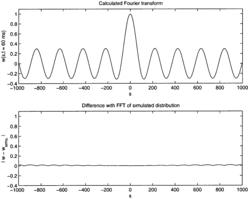
We have run a Monte-Carlo simulation, with particles starting at the origin, and with equal probability to start leftward and rightward. At each time step, a random trial decides if a particle changes its speed, in accordance with the Poisson distribution. The time step is chosen small enough to avoid a significant bias in the distribution of the instants of changes, when time is sampled. At a given date t, the simulation is stopped, and the particles are counted in each interval [Xk, Xk+1)

of the space domain. The (fast) Fourier transform of the resulting density is compared to the exact solution on figure (1-2). The distribution obtained from the simulation is also plotted on figure (1-3). The two sharp peaks are clearly visible.

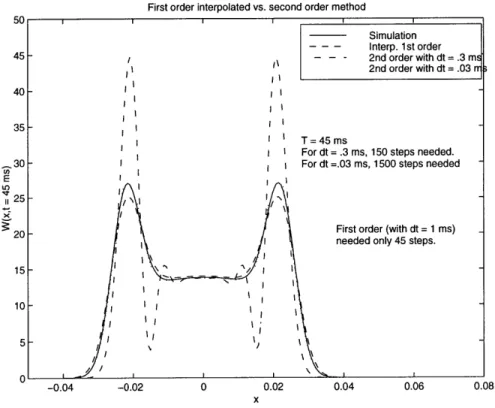
We also solved the partial differential equation (1.31) numerically, by a standard first order forward Euler scheme. A comparison of the numerical solution with the simulation is plotted on figure (1-4). In this case, the initial distribution was Gaussian; this explains the significant extension of the two peaks. Higher order forward Euler schemes were then studied, with no significant improvement. On the contrary, instability was a reason for increasing the number of iterations needed. The figure (1-5) shows these results.

In all cases, the following values were chosen :

(31)

Calculated Fourier transform

Difference with FFT of simulated distribution

-600 -400 -200 0 200 400 600 800 1000

Figure 1-2: Top : exact Fourier transform of the distribution. Bottom of the distribution obtained by a Monte-Carlo simulation.

: Comparison with the FFT

Distnbution evaluated by Monte-Carlo simulation 600 500 400 is 300 2T 200 100 0 -4 -3 -2 -1 0 1 2 3 4 x In cm

Zoom on the central values (no filtenng)

25 20 W 15 10 5 -4 -3 -2 -1 0 x in cm 2 3

Figure 1-3: Distribution obtained from the simulation. The roughness of the curve shown on bottom is due to the use of a finite number of particles (smoothness improves as this number increases).

-0.2 -0.4 -1000 -800 0.8 0.6 I I I 1 I I I I I

(32)

T = 45 ms

Figure 1-4: Comparison between the distribution obtained from the simulation and a numerical resolution of the differential equations (1.31). The initial distribution is a Gaussian (hence "fatter" peaks).

First order interpolated vs. second order method

E

25

20

-0.04 -0.02 0 0.02 0.04 0.06 0.08

Figure 1-5: Comparisons between various cases of the Euler of the second order method, with too large a time step.

(33)

Chapter 2 Probabilistic models for air traffic

control

2.1 Modeling uncertainty

We may apply the framework shown in the previous chapter to the case of air traffic control, where the behaviours of pilots and aircraft can be described in terms of probability. Poisson processes play a key-role in this context, conveniently modeling events occurring with a mean frequency A.

In the following, we use the model and the assumptions proposed earlier [6, 1, 17]. In particular, the planes are treated by pairs host/intruder, where the host has a well-known probabilistic behaviour while the intruder may take unexpected actions. The main issue of the modeling is to compute

WH(x, t) and W (x, t), the respective probability density functions of the host and the intruder - in

fact, their evolution in time and space, as described by integro-differential equations, but also the probability of collision for the pair, as defined in [6].

Let us assume the host is flying with initial heading H, at altitude hH and initial position

(XH, YH) at that altitude. We denote 0I, hi, and (xI, yl) the corresponding variables for the intruder. We now briefly recall the model used. Each plane has a nominal speed, with fluctuations assumed to be Gaussian, with standard deviation a, = 15 kts. Only the along-track position is affected by these fluctuations. The speed, though imperfectly known, is assumed to remain the same along the trajectory. The cross-track position is also not completely deterministic, and is assumed to be normally distributed with standard deviation actp = 1 nmi. The imperfect knowledge of the intruder's behaviour is modeled as follows : the plane may engage changes of altitude with a mean frequency of A = 4 h-1, as well as changes of heading with the same mean frequency. When changing of altitude, the final altitude is random, with uniform distribution between 0 and 10, 000 ft. The heading changes do not have a uniform distribution, but favor left or right turn between 5 and 20

(34)

degrees. In case of high collision risk, controllers may submit orders to the pilots of the host airplane, orders to be executed after a random time following a gamma distribution with mean 1 min and such that the orders are executed within 2 min with 95% probability (flight crew response latency)

[17]. The action to take may also be suggested by an automatic system of conflict alert, aboard. As

in this paragraph, we will use the subscript H for the flight parameters of the host aircraft, and the subscript I for the intruder.

We now construct the system of equations the probability density function should satisfy, follow-ing step by step the procedure described above : first derive the Fokker-Planck equation of a plane with fixed heading and altitude, second add exchange terms to obtain the system.

The variables of the problem have to split into two different groups : the variables (x, y), with Gaussian distributions, and the variables driven by Poisson processes, namely 0 and h. Observing that a plane with fixed

4

and h has a well-known (probabilistic) trajectory, we will consider from now on a continuous set of systems EP,h modeling the aircraft with heading 7 and altitude h. The possible values of the altitude are equally distributed over [0, 10, 000 ft]. In the system EP,h,

according to the model the aircraft follows the stochastic differential equation :

dXt = VH,I (dt + dWt,) (2.1)

IVH,II

where VH,I denotes the vector speed, and dWt/cl, the one-dimensional Standard Brownian Motion'. The constant c represents the time unit, playing the role of a scaling factor; in our context, c =

1 h. The nominal speed is assumed horizontal, ie with coordinates VH,I = vH,I (cos

4,

sin

4,

0). The linear, differential equation (2.1) leads to the following Fokker-Planck equation for system

(¢, h)[4, 15] :

(X, h, t) = -VH '.VW h(X, h, t) + V.B VW¢'h(X, h, t) (2.2)

at 2

where X = (x, y), a2 = col2, and B is the 2 x 2 symmetric, diffusion matrix

B cos24' sin4 cos4)

= sin 4 cos 4 sin2 4'

Observe that B = u uT, if u stands for the unit vector VH,I/IVH,II with 2D-coordinates (cos

4,

sin

4).

1

As in the previous chapter, this refers to a Gaussian process with mean and standard deviation proportional to time. The coefficients of proportionality, called drift rate for the mean and variance rate for the standard deviation, are respectively 0 and 1 in arbitrary units in the case of Standard Brownian Motion. The abstract process must be scaled by physical constants to obtain a physical process, in particular a length for the standard deviation and a speed for the drift rate. This is the role of the constant c.

(35)

The last term of equation (2.2), multiplied by a2/2 is thus a short-hand for :

02W O2W 2 W ( 0)

9

2

cos2 + 2 sin 4 coso y + sin2 y cos ? ix +

sin 0y W

In equation (2.2), the redundant superscript h is used to recall that the altitude is a random variable with Poisson behaviour, and hence deserves a particular treatment.

Also, space derivations do not hold for the altitude h. The first order term is traditionally called the drift term. The second order term is known as a diffusion term (hence the name of diffusion matrix for B). The uncertainty in cross-track position can be taken into account in the initial distribution WA'h(X, h, t = 0).

We now have to state what exchange rates the model imposes here. As for the intruder, we have

Intruder: A( ,h -+ ',h')(t) = A k(4' -

4)

u(h)

where k(O) is the probability density function used by Yang and Kuchar to describe the preferred angle of turn, and u(h) the uniform distribution over the possible altitudes h. Thus, u(h) is a constant that will be denoted U. Note that the function k(O) is even.

The relations of the transfer coefficients A(V, h -+ 0', h')(t) to the model are very intuitive :

during dt, the probability to change the heading from

4

to

4'

and the altitude from h to h' is

k(0' -4) u(h) - since the altitude h is a uniformly distributed random variable. But this probability has to be multiplied by that of the actual decision to maneuver, namely A dt. Hence the coefficients for the intruder.

Now, for the host, suppose the maneuver thought of to prevent from collision is a left turn of ¢ degrees from present heading, at a constant altitude hH. Then only two headings are of concern, 4'H and OH + ¢, and we only have to describe the transition between these two angles. We then consider

only WC H,hH and W 'H+OhH, and the corresponding transfer coefficient A(OH, hH -+ OH- + , hH)(t). If to denotes the time when pilots are notified to take action, we have

A(OH,hH -+ OH + -, hH)(t) { before to

A y(t - to) after to

All other transfer coefficients are zero - including A(4H + 0, hH -+ OH, hH)(t) (pilots do not turn right back). Remark that the instant to, which may be seen as an instant of switch between two models, is entirely determined by the security system (or the controller). But in turn this is an independent event (intruder plane continuing on dangerous action) that determines the decision of the system (the controller). The host is not a closed-loop system.

Differential Kolmogorov equations for transiting processes

Differential Kolmogorov Equations for Transiting Processes

by

Gael D6silles

Ingenieur Dipl6me de l'Ecole Polytechnique, France (1995)

Ing6nieur Dipl6m6 de l'Ecole Nationale Superieure de 1'Aeronautique et de l'Espace,

France (1997)

Submitted to the Department of Aeronautics and Astronautics

in partial fulfillment of the requirements for the degree of

Master of Science

at the

MASSACHUSETTS INSTITUTE OF TECHNOLOGY

June 1998

) Massachusetts Institute of Technology 1998. All rights reserved.

Author

.

...

...

...

Department of Aeronautics and Astronautics

April 1998

7/

Certified by ...

...

Eric Feron

Assistant Professor

Thesis Supervisor

Accepted

by...

...

...

..

Chairman, Department Committeb on Graduate Student

JUL

087~8

Differential Kolmogorov Equations for Transiting Processes

by

Gael D6silles

Abstract

Acknowledgements

Contents

List of Figures

Introduction

Chapter 1

Differential Kolmogorov equation

for transiting Markov processes

1.1

Position of the problem, Notations

}

1.2

Practical treatment

1.2.1

Expansion of the conditional density functions

I

1.2.2

Evolution of the masses

j

1.3

Extension to a continuum of systems

1.3.1

Writing the equations in the continuous parameter

}

W

IA

I

Sd/oP{x(t')

p,

1.3.2

Redundancy of the definitions

f

Pa

W(x,t) =

WA (x, t)

p)

1.4

Discussion

f

1.4.1

Structure of the Kolmogorov equations

f

_aw

_{+ A}

_{(W - W}

_{- )}

_{= A (p- -+)}